Wave Exciting Force Maximization of Truncated Cylinders in a Linear Array


Abstract
:1. Introduction
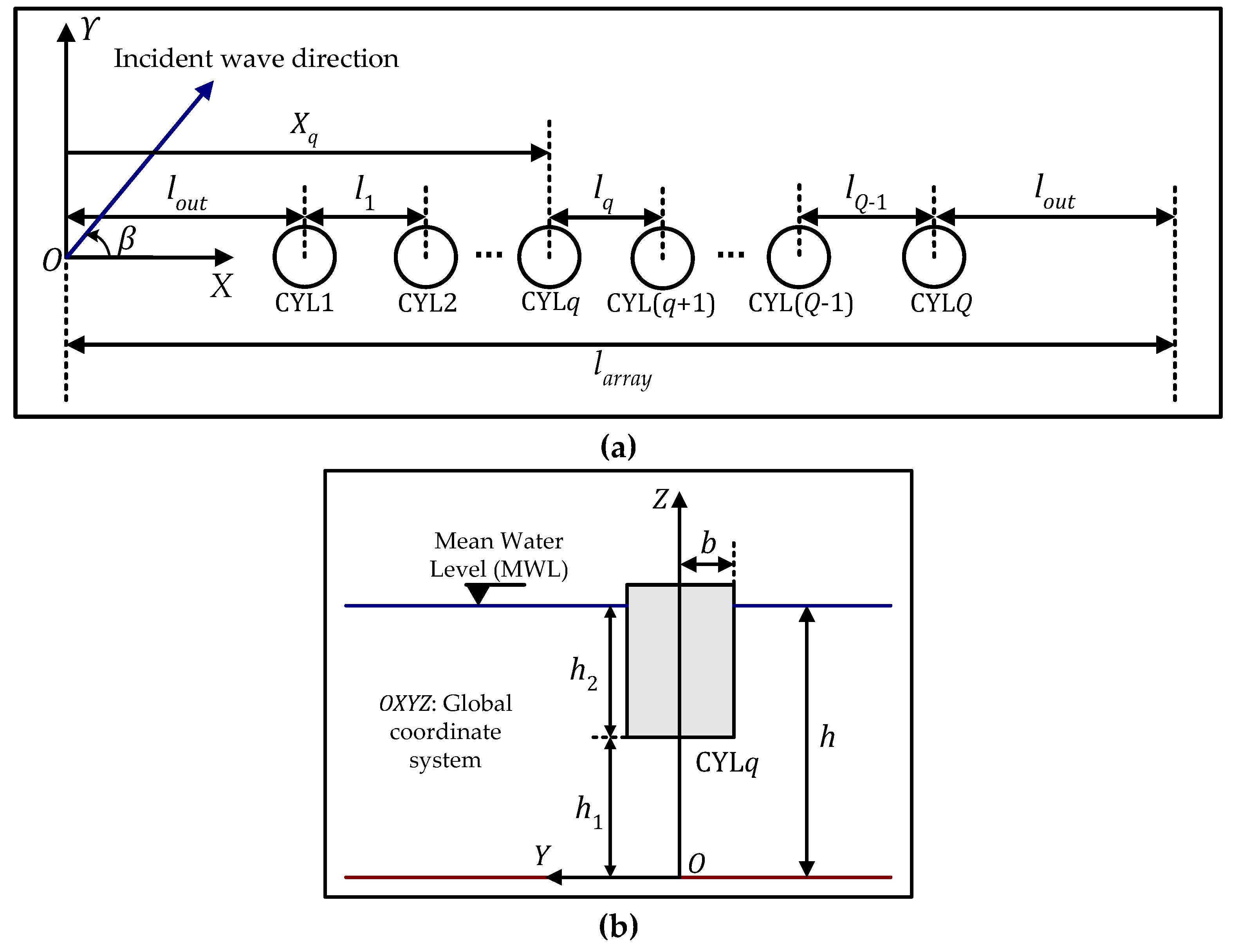
2. Problem’s Definition
3. Numerical Modeling
3.1. Hydrodynamic Model
3.2. Genetic Algorithms Solver
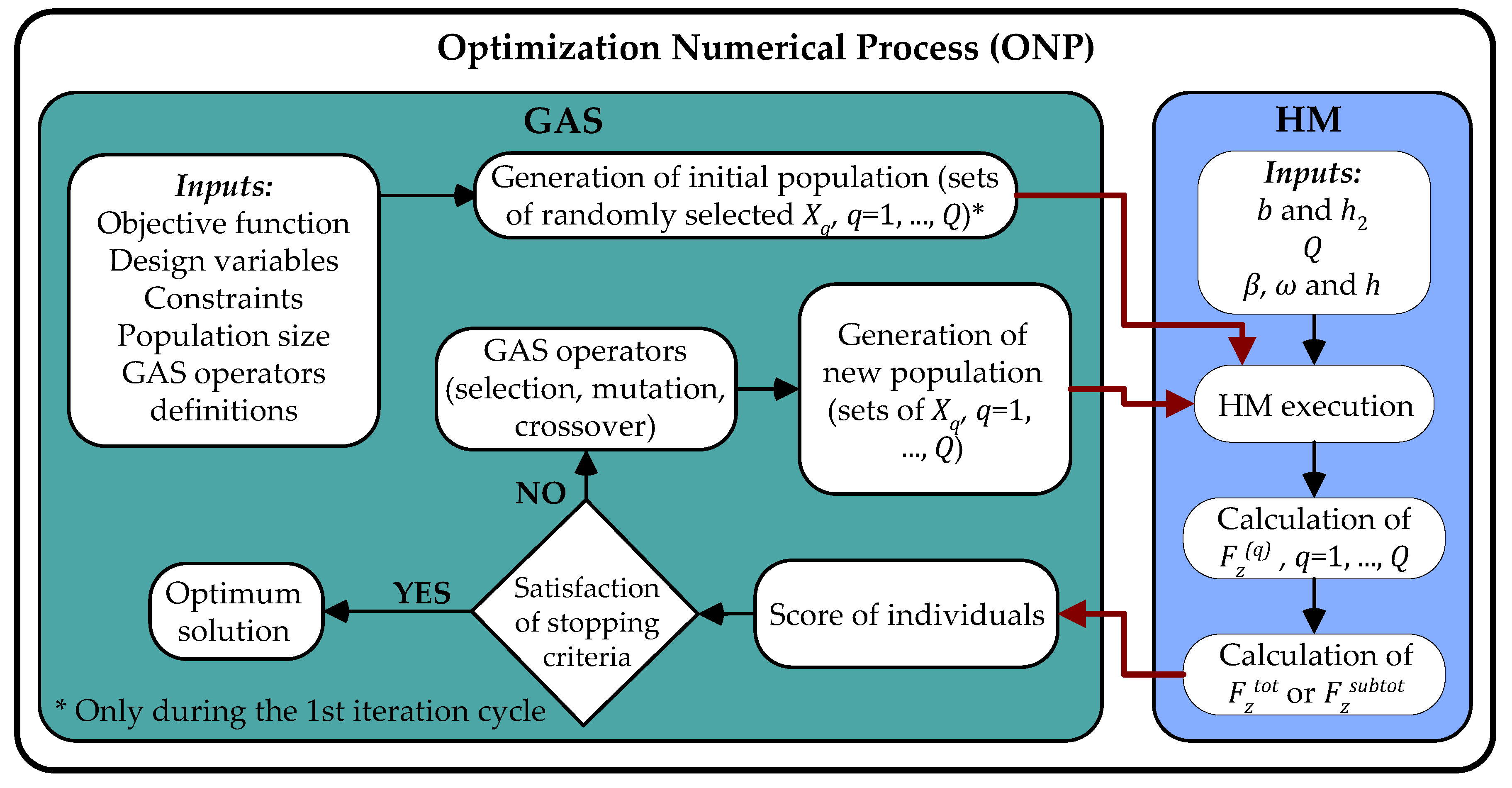
3.3. Optimization Numerical Process (ONP)
4. ONP Validation
5. Results and Discussions
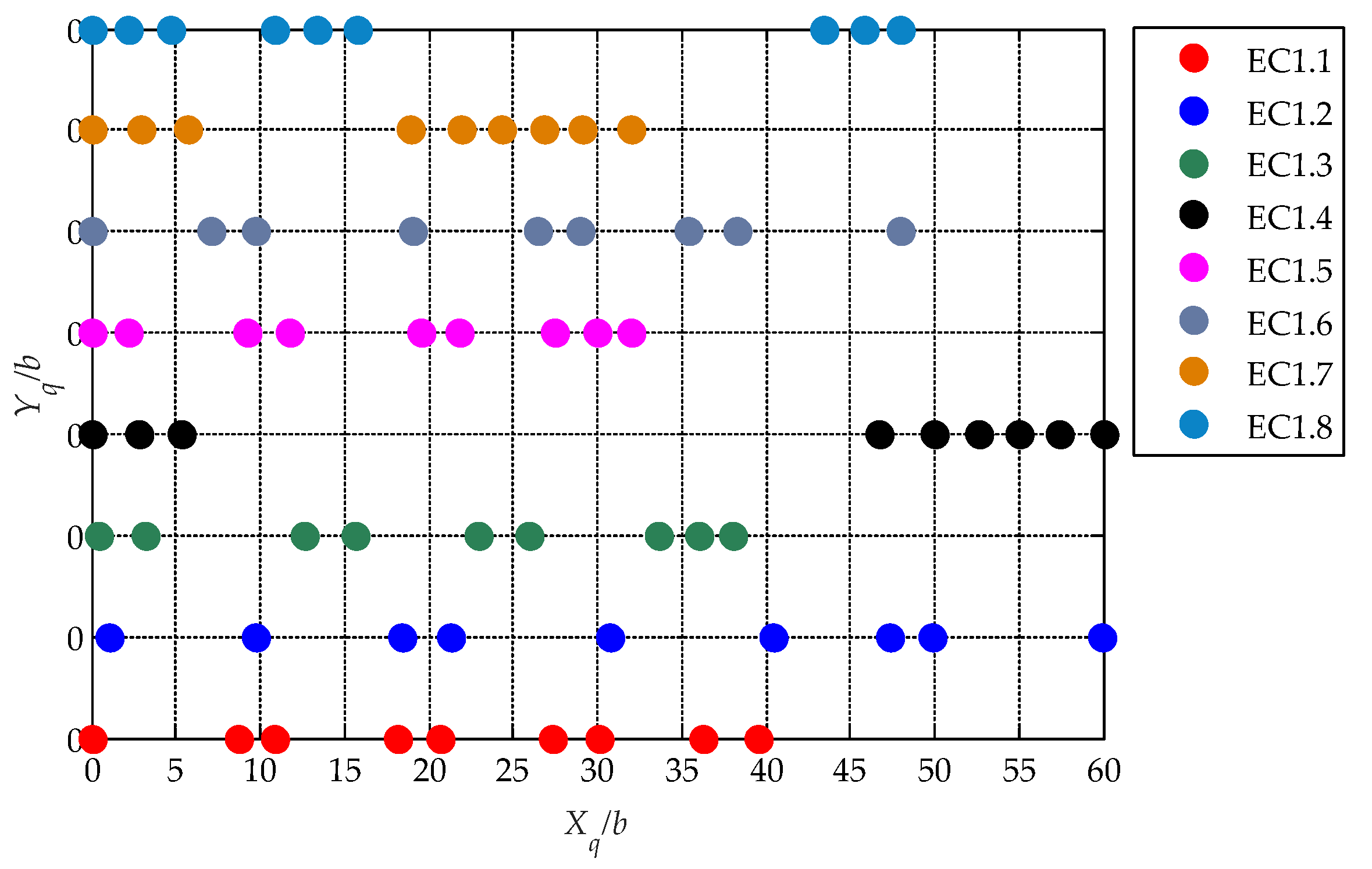
5.1. Examined Cases
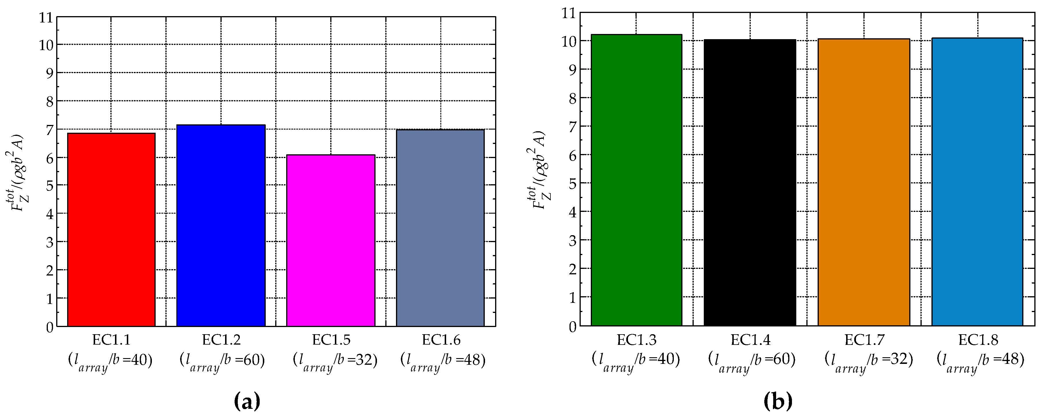
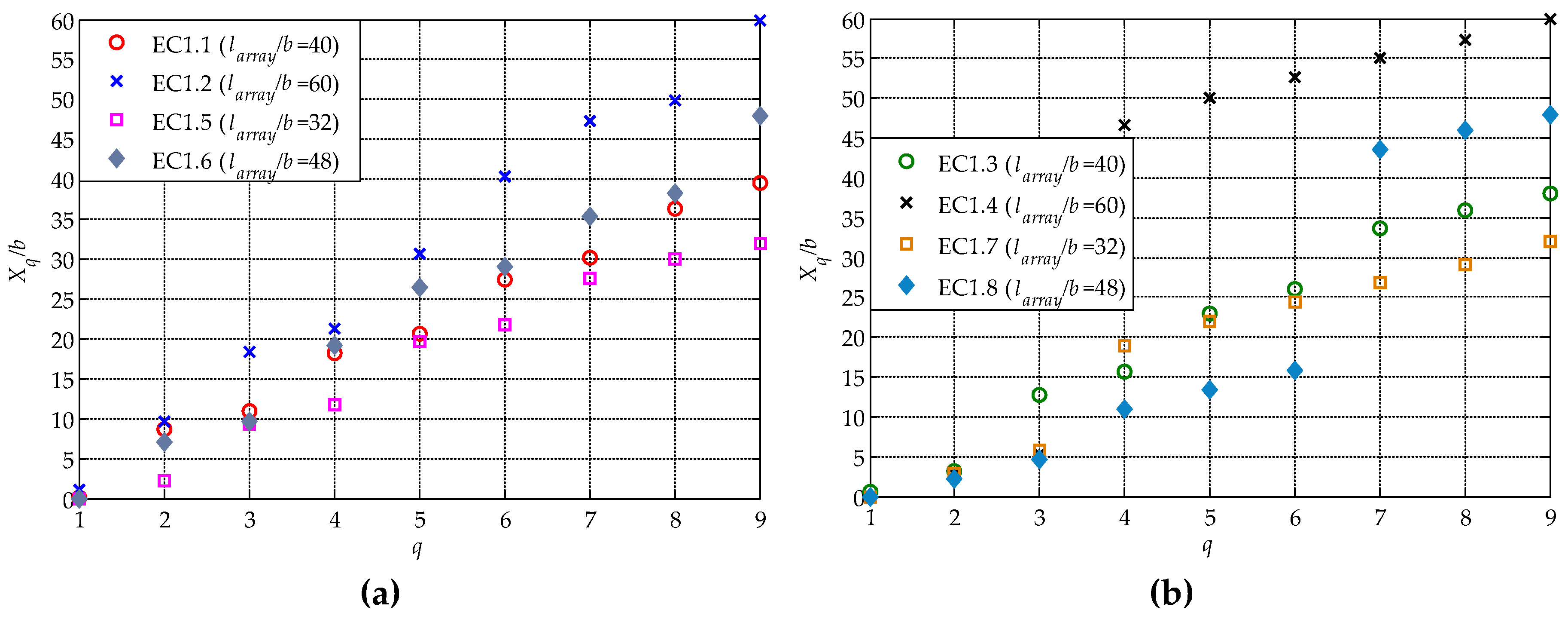
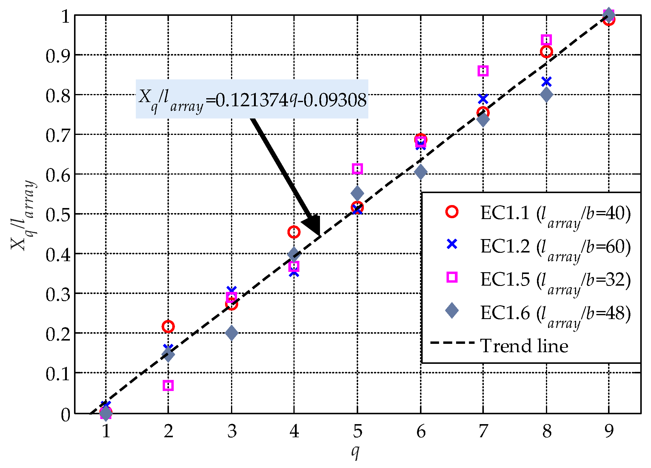
5.2. Optimum Solutions for EC1.1–EC1.8
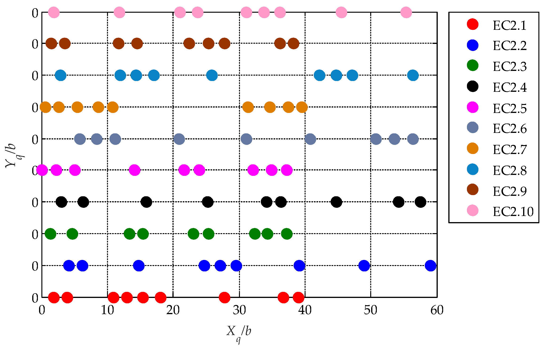
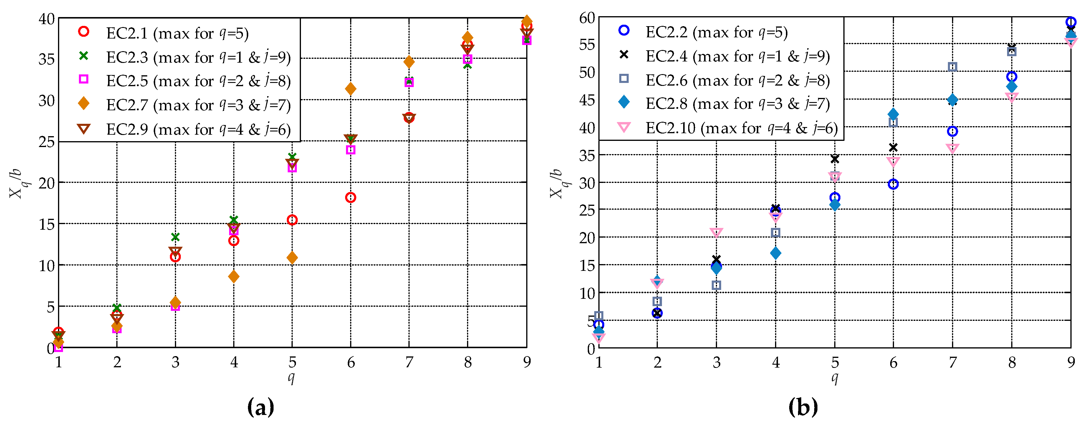
5.3. Optimum Solutions for EC2.1–EC2.10
6. Conclusions
Author Contributions
Funding
Conflicts of Interest
References
- Ohkusu, M. Hydrodynamic forces on multiple cylinders in waves. In Proceedings of the International Symposium on Dynamics of Marine Vehicles and Structures in Waves, London, UK, 1–5 April 1974; pp. 107–112. [Google Scholar]
- Kagemoto, H.; Yue, D.K.P. Interactions among multiple three-dimensional bodies in water waves: An exact algebraic method. J. Fluid Mech. 1986, 166, 189–209. [Google Scholar] [CrossRef]
- Yilmaz, O.; Incecik, A. Analytical solutions of the diffraction problem of a group of truncated vertical cylinders. Ocean Eng. 1998, 25, 385–394. [Google Scholar] [CrossRef]
- Chatjigeorgiou, I.K. Analytical Methods in Marine Hydrodynamics; Cambridge University Press: Cambridge, UK, 2018. [Google Scholar]
- Williams, A.N.; Demirbilek, Z. Hydrodynamic interactions in floating cylinder arrays—I. Wave scattering. Ocean Eng. 1988, 15, 549–583. [Google Scholar] [CrossRef]
- Garnaud, X.; Mei, C.C. Bragg scattering and wave-power extraction by an array of small buoys. Proc. R. Soc. A 2010, 466, 79–106. [Google Scholar] [CrossRef] [Green Version]
- Kashiwagi, M. Wave scattering among a large number of floating cylinders. Struct. Eng. Mech. 2005, 21, 53–66. [Google Scholar] [CrossRef]
- Siddorn, P.; Eatock Taylor, R. Diffraction and independent radiation by an array of floating cylinders. Appl. Ocean Res. 2008, 35, 1289–1303. [Google Scholar] [CrossRef]
- Wolgamot, H.A.; Eatock Taylor, R.; Taylor, P.H. Radiation, trapping and near trapping in arrays of floating truncated cylinders. J. Eng. Math. 2015, 9, 17–35. [Google Scholar] [CrossRef]
- Chatjigeorgiou, I.K.; Chatziioannou, K.; Mavrakos, T. Near trapped modes in a long array of truncated circular cylinders. J. Water. Port C.-ASCE 2019, 145, 04018035. [Google Scholar] [CrossRef]
- Kagemoto, H. Minimization of wave forces on an array of floating bodies—The inverse hydrodynamic interaction theory. Appl. Ocean Res. 1992, 14, 83–92. [Google Scholar] [CrossRef]
- Fletcher, R.; Powell, M.J.D. A rapidly convergent descent method for minimization. Comput. J. 1963, 6, 163–168. [Google Scholar] [CrossRef]
- Fiacco, A.V.; McCormick, G.P. Nonlinear Programming: Sequential Unconstrained Minimization Techniques; John Wiley & Sons: New York, NY, USA, 1968. [Google Scholar]
- Deb, K. Multi-Objective Optimization Using Evolutionary Algorithms; John Wiley & Sons: New York, NY, USA, 2001. [Google Scholar]
- Holland, J.H. Adaptation in Natural and Artificial Systems; MIT Press: Cambridge, MA, USA, 1975. [Google Scholar]
- Tasrief, M.; Kashiwagi, M. Improvement of ship geometry by optimizing the sectional area curve with binary-coded genetic algorithms (BCGAS). In Proceedings of the 23th International Offshore and Polar Engineering Conference (ISOPE 2013), Anchorage, AK, USA, 30 June–5 July 2013; pp. 869–875. [Google Scholar]
- Iida, T.; Kashiwagi, M.; He, G. Numerical confirmation of cloaking phenomenon array of floating bodies and reduction of wave drift force. Int. J. Offshore Polar Eng. 2014, 24, 241–246. [Google Scholar]
- Zhang, Z.; He, G.; Wang, Z. Real-coded genetic algorithm optimization in reduction of wave drift forces on an array of truncated cylinders. J. Mar. Sci. Technol. 2019, 24, 930–947. [Google Scholar] [CrossRef]
- Loukogeorgaki, E.; Kashiwagi, M. Minimization of drift force on a floating cylinder by optimizing the flexural rigidity of a concentric annular plate. Appl. Ocean Res. 2019, 85, 136–150. [Google Scholar] [CrossRef]
- Michailides, C.; Angelides, D.C. Optimization of a flexible floating structure for wave energy production and protection effectiveness. Eng. Struct. 2015, 85, 249–263. [Google Scholar] [CrossRef]
- Gao, R.P.; Wang, C.M.; Koh, C.G. Reducing hydroelastic response of pontoon-type very large floating structures using flexible connector and gill cells. Eng. Struct. 2013, 52, 372–383. [Google Scholar] [CrossRef]
- Child, B.F.M.; Venugopal, V. Optimal configurations of wave energy device arrays. Ocean Eng. 2010, 37, 1402–1417. [Google Scholar] [CrossRef]
- Ruiz, P.M.; Nava, V.; Topper, M.B.R.; Minguela, P.R.; Ferri, F.; Kofoed, J.P. Layout optimization of wave energy converter arrays. Energies 2017, 10, 1262. [Google Scholar] [CrossRef] [Green Version]
- Sharp, C.; DuPont, B. Wave energy converter array optimization: A genetic algorithm approach and minimum separation distance study. Ocean Eng. 2018, 163, 148–156. [Google Scholar] [CrossRef]
- Chatjigeorgiou, I.K. Water wave trapping in a long array of bottomless circular cylinders. Wave Motion 2018, 83, 25–48. [Google Scholar] [CrossRef]
- MATLAB Optimization Toolbox R2019b. version 9.7.0.1261785 (R2019b) Update 3. The MathWorks, Inc.: Natick, MA, USA.
- MATLAB R2019b. version 9.7.0.1261785 (R2019b) Update 3. The MathWorks, Inc.: Natick, MA, USA.
- Loukogeorgaki, E.; Chatjigeorgiou, I.K. Hydrodynamic Performance of an Array of Wave Energy Converters in Front of a Vertical Wall. In Proceedings of the 13th European Wave and Tidal Energy Conference (EWTEC 2019), Napoli, Italy, 1–6 September 2019. Paper No. 1464. [Google Scholar]


| ONP | Kagemoto [11] | |||||
|---|---|---|---|---|---|---|
| - | - | |||||
| Case | Objective Function | |||
|---|---|---|---|---|
| EC1.1 | Maximization of with in Equation (26) | |||
| EC1.2 | ||||
| EC1.3 | ||||
| EC1.4 | ||||
| EC1.5 | ||||
| EC1.6 | ||||
| EC1.7 | ||||
| EC1.8 | ||||
| EC2.1 | Maximization of for and in Equation (27) | |||
| EC2.2 | ||||
| EC2.3 | Maximization of for and in Equation (27) | |||
| EC2.4 | ||||
| EC2.5 | Maximization of for and in Equation (27) | |||
| EC2.6 | ||||
| EC2.7 | Maximization of for and in Equation (27) | |||
| EC2.8 | ||||
| EC2.9 | Maximization of for and in Equation (27) | |||
| EC2.10 |
| Case | ||||||||||
|---|---|---|---|---|---|---|---|---|---|---|
| EC1.1 | 0.10 | 8.70 | 10.90 | 18.20 | 20.70 | 27.40 | 30.10 | 36.30 | 39.50 | 6.841 |
| EC1.2 | 1.10 | 9.70 | 18.40 | 21.30 | 30.70 | 40.40 | 47.30 | 49.90 | 59.90 | 7.137 |
| EC1.3 | 0.50 | 3.20 | 12.70 | 15.60 | 22.90 | 26.00 | 33.60 | 36.00 | 38.10 | 10.212 |
| EC1.4 | 0.00 | 2.80 | 5.30 | 46.70 | 50.00 | 52.70 | 55.00 | 57.40 | 60.00 | 10.017 |
| EC1.5 | 0.00 | 2.20 | 9.30 | 11.80 | 19.60 | 21.80 | 27.50 | 30.00 | 32.00 | 6.075 |
| EC1.6 | 0.00 | 7.10 | 9.70 | 19.10 | 26.50 | 29.00 | 35.40 | 38.30 | 48.00 | 6.968 |
| EC1.7 | 0.00 | 2.90 | 5.70 | 18.90 | 21.90 | 24.40 | 26.80 | 29.10 | 32.00 | 10.035 |
| EC1.8 | 0.00 | 2.20 | 4.70 | 10.90 | 13.40 | 15.80 | 43.50 | 45.90 | 48.00 | 10.090 |
| Case | ||||||||||
|---|---|---|---|---|---|---|---|---|---|---|
| EC2.1 | 1.80 | 3.90 | 10.90 | 12.90 | 15.40 | 18.10 | 27.80 | 36.70 | 39.00 | 1.5854 |
| EC2.2 | 4.20 | 6.20 | 14.70 | 24.70 | 27.10 | 29.60 | 39.10 | 49.00 | 59.00 | 1.6066 |
| EC2.3 | 1.40 | 4.70 | 13.40 | 15.40 | 23.10 | 25.30 | 32.30 | 34.30 | 37.20 | 2.5921 |
| EC2.4 | 3.00 | 6.30 | 15.90 | 25.20 | 34.10 | 36.30 | 44.70 | 54.20 | 57.50 | 2.5742 |
| EC2.5 | 0.00 | 2.20 | 5.00 | 14.10 | 21.70 | 23.90 | 32.10 | 34.90 | 37.20 | 2.7583 |
| EC2.6 | 5.80 | 8.40 | 11.20 | 20.90 | 31.10 | 40.80 | 50.80 | 53.60 | 56.30 | 2.7670 |
| EC2.7 | 0.60 | 2.60 | 5.40 | 8.60 | 10.80 | 31.30 | 34.60 | 37.50 | 39.50 | 2.7262 |
| EC2.8 | 2.90 | 11.90 | 14.30 | 17.10 | 25.90 | 42.20 | 44.80 | 47.20 | 56.40 | 2.8065 |
| EC2.9 | 1.50 | 3.50 | 11.70 | 14.50 | 22.40 | 25.30 | 27.80 | 36.20 | 38.20 | 2.8033 |
| EC2.10 | 1.90 | 11.80 | 21.00 | 23.70 | 31.10 | 33.80 | 36.20 | 45.50 | 55.40 | 2.8618 |
| Case | ||||||||||
|---|---|---|---|---|---|---|---|---|---|---|
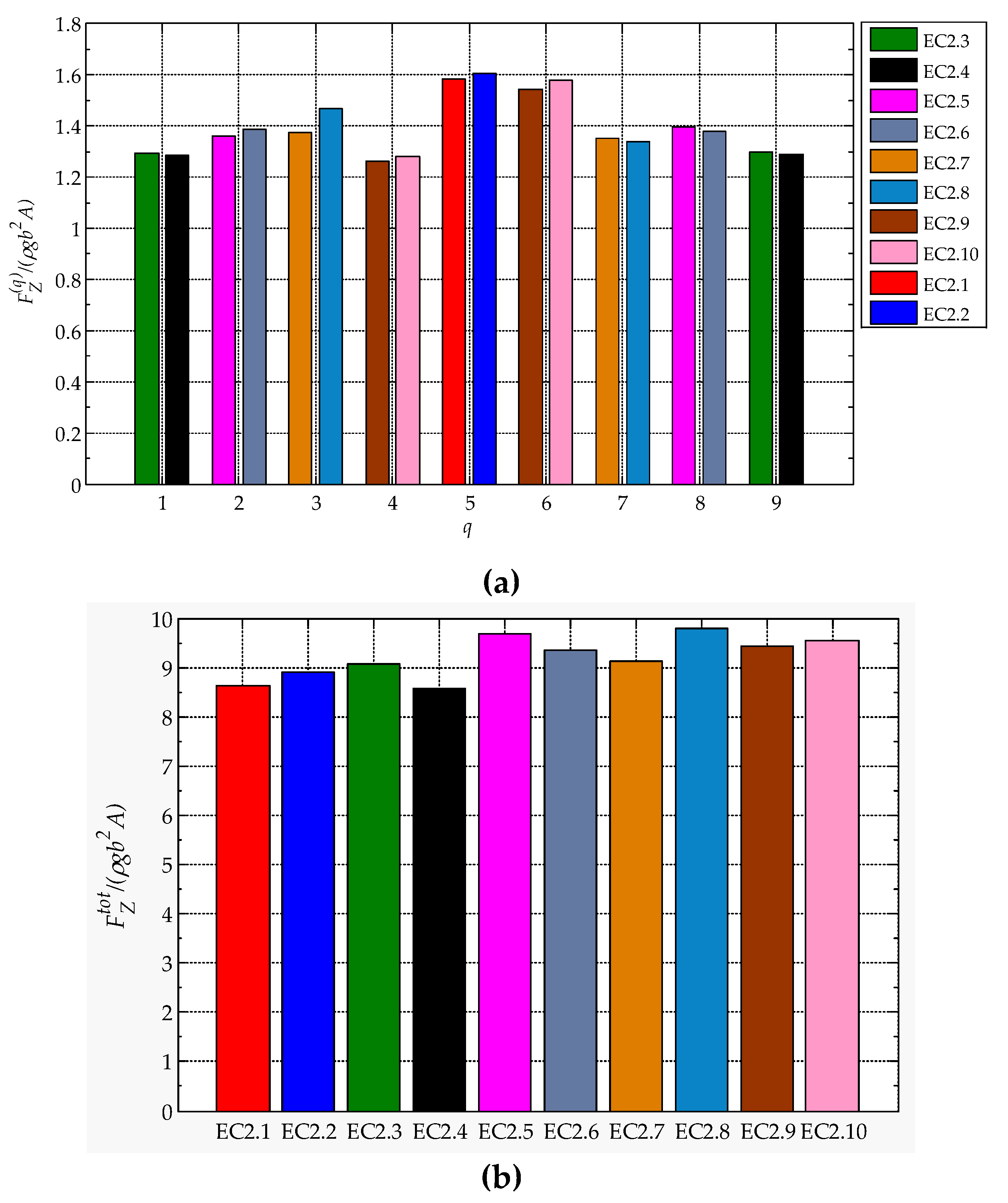
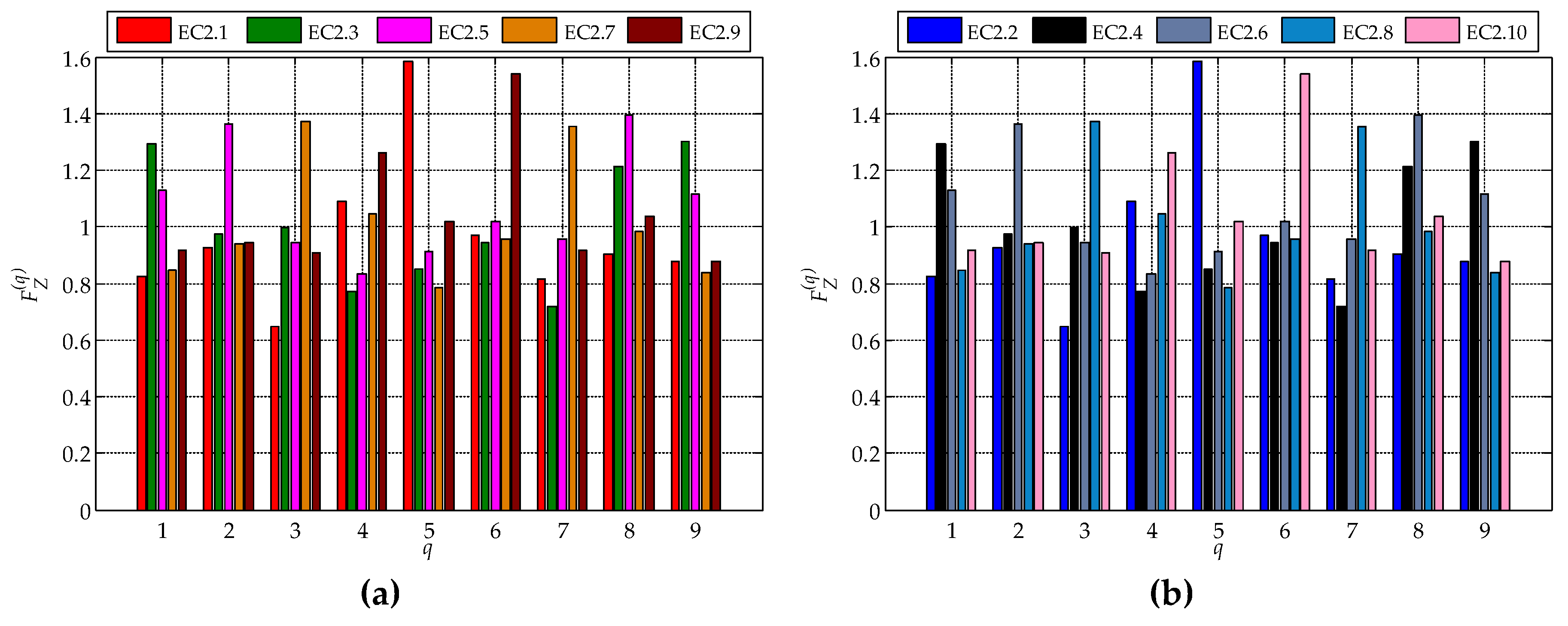
| EC2.1 | 0.8226 | 0.9252 | 0.6471 | 1.0907 | 1.5854 | 0.9715 | 0.8162 | 0.9043 | 0.8791 | 8.6421 |
| EC2.2 | 0.8574 | 0.9521 | 0.8326 | 1.0353 | 1.6066 | 1.0241 | 0.9176 | 0.8459 | 0.8345 | 8.9062 |
| EC2.3 | 1.2923 | 0.9728 | 0.9957 | 0.7696 | 0.8527 | 0.9442 | 0.7182 | 1.2133 | 1.2998 | 9.0586 |
| EC2.4 | 1.2844 | 0.9606 | 0.7900 | 0.7714 | 0.8406 | 0.9169 | 0.7725 | 0.9369 | 1.2897 | 8.5631 |
| EC2.5 | 1.1283 | 1.3630 | 0.9451 | 0.8343 | 0.9146 | 1.0193 | 0.9563 | 1.3954 | 1.1155 | 9.6716 |
| EC2.6 | 1.0812 | 1.3888 | 0.9813 | 0.8426 | 0.8016 | 0.8232 | 0.9905 | 1.3782 | 1.0650 | 9.3523 |
| EC2.7 | 0.8450 | 0.9402 | 1.3724 | 1.0471 | 0.7847 | 0.9590 | 1.3538 | 0.9844 | 0.8380 | 9.1245 |
| EC2.8 | 1.0085 | 1.0164 | 1.4672 | 0.9892 | 0.9476 | 1.0915 | 1.3393 | 0.9905 | 0.9495 | 9.7998 |
| EC2.9 | 0.9191 | 0.9416 | 0.9061 | 1.2613 | 1.0189 | 1.5420 | 0.9170 | 1.0359 | 0.8775 | 9.4195 |
| EC2.10 | 0.9050 | 0.9024 | 0.9690 | 1.2821 | 0.9843 | 1.5796 | 1.0082 | 0.9658 | 0.9381 | 9.5347 |
© 2020 by the authors. Licensee MDPI, Basel, Switzerland. This article is an open access article distributed under the terms and conditions of the Creative Commons Attribution (CC BY) license (http://creativecommons.org/licenses/by/4.0/).
Share and Cite
Michailides, C.; Loukogeorgaki, E.; Chatjigeorgiou, I.K. Wave Exciting Force Maximization of Truncated Cylinders in a Linear Array. Energies 2020, 13, 2400. https://doi.org/10.3390/en13092400
Michailides C, Loukogeorgaki E, Chatjigeorgiou IK. Wave Exciting Force Maximization of Truncated Cylinders in a Linear Array. Energies. 2020; 13(9):2400. https://doi.org/10.3390/en13092400
Chicago/Turabian StyleMichailides, Constantine, Eva Loukogeorgaki, and Ioannis K. Chatjigeorgiou. 2020. "Wave Exciting Force Maximization of Truncated Cylinders in a Linear Array" Energies 13, no. 9: 2400. https://doi.org/10.3390/en13092400