Time-Varying Relationship between Crude Oil Price and Exchange Rate in the Context of Structural Breaks

Abstract

This paper examines the dynamic relationship between crude oil prices and the U.S. exchange rate within the structural break detection context. Based on monthly data from January 1996 to April 2019, this paper identifies structural breaks in movements of oil price and examines the dynamic relationship between crude oil prices and the U.S. exchange rate movement by introducing the economic policy uncertainty and using the TVP-VAR (Time-Varying Parameter-Vector Auto Regression ) model. Empirical results indicate that shocks to crude oil prices have immediate and short-term impacts on movements in the exchange rate which are emphasized during the confidence intervals of structural breaks. Oil price shocks and economic policy uncertainty are interrelated and influence movements in the U.S. exchange rate. Since the U.S. dollar is the main currency of the international oil market and the U.S. has become a major exporter of crude oil, the transmission of price shocks to the U.S. exchange rate becomes complicated. In most cases, the relationship between oil prices and the U.S. exchange rate movements is negative.

1. Introduction

The fluctuation of oil prices has an important influence on a country’s exchange rate. Crude oil is the main energy source in the world and its price does not have significant arbitrage space in the global scope, while the exchange rate is the price link connecting the internal and external economy. Therefore, in a market-oriented and open economy, the fluctuation of crude oil prices will cause the change of an economy’s exchange rate. Relevant literature proves that the fluctuation of crude oil prices will cause the exchange rate of USD to move in the same direction of the oil-importing countries, such as China [1,2,3,4,5]. For oil-importing countries, oil price fluctuations constitute the main source of exogenous shocks to a country’s economy and also have an important impact on the exchange rate of importing countries [6,7,8]. Similarly, for crude oil, there is a long-term equilibrium relationship between oil price and exchange rate [9,10]. At the same time, when the crude oil price volatility is incorporated into the corresponding currency or asset selection model, the oil price volatility has a significant impact on the exchange rate. For example, Coudert and Mignon [11] added oil price volatility into the currency model and found that the increase of oil price would lead to the depreciation of the importing country’s currency. Kumar [12] built an asset selection model by introducing capital account opening and found that the decline of crude oil price had a significant long-term negative impact on the RMB exchange rate, which varied with the degree of capital account opening.

The impact of oil price fluctuation on exchange rates is time-varying. The time variability of the impact on the exchange rate by the rise or fall of crude oil prices has a strong correlation with the non-linear or asymmetric mechanism of the impact. It is also affected by the mood and behavior of investors in the financial market [13,14,15,16,17]. Monetary policies strengthened the impact of oil price shock on the macro-economy, and the impact of oil price shock on exchange rate fluctuations showed non-linear characteristics in this process [18,19,20]. The impact of oil prices on China’s macro-economy and the exchange rate is significantly positive, and it is an asymmetric one-way impact [21]. Different exchange rate regime arrangements are an important source of heterogeneous impact of oil price fluctuations on exchange rate [22]. It can be seen that the degree of co-movement between crude oil price and exchange rate varies with time. Some researchers confirmed this conclusion by using the wavelet coherent framework [23,24].

The influence of oil price on the exchange rate is different in time length. From the perspective of the trend of exchange rate price fluctuation, the influential factors of the long-term, medium-term and short-term frequency are different. In the long-run, exchange rate is more affected by fundamentals, such as macroeconomic environment, etc., so the exchange rate tends to equilibrium price in the long term [25,26]. In the short term, the exchange rate is more influenced by technical aspects, such as the early trend of the exchange rate and the relationship between volume and price in the transaction. In the process of the impact of oil price on exchange rate, there are a series of transmission variables, which may be influencing factors in different periods, so the time length of oil price’s impact on exchange rate is different [27].

The influence of crude oil price on exchange rate is strongly related to crude oil price breaks. Crude oil price fluctuations are affected from different levels, some of which are long-term shocks, some of which are short-term shocks. The nature of shocks is not exactly the same, as some belong to policy changes, while some belong to sudden events. The complexity of the causes of crude oil price fluctuations, especially the sudden events, will produce breaks for crude oil price fluctuations [28,29,30,31]. Therefore, the correlation between the impact of crude oil price on the exchange rate and the breaks of crude oil price is strengthened due to the difference between the influence factors such as the breaks of crude oil price and the influence factors of the trend change. In addition, the impact of crude oil price on exchange rate also shows asymmetry [32], and there is a significant, two-way, nonlinear Granger causality between crude oil price and exchange rate [33].

Above all, the analysis makes several significant contributions in three folds. Firstly, the time-varying dynamic relationship between crude oil price and exchange rate fluctuation is investigated, and the uncertainty of economic policy is introduced into the analysis. The existing literature mainly analyzes the static relationship between crude oil price fluctuation and exchange rate volatility, with some focus on the risk spillover between the two [34,35,36]. This paper considers the dynamic relationship between the two, which is more in line with the time-varying characteristics, and it introduces the uncertainty of American economic policies. Secondly, the influence of crude oil price on exchange rate fluctuation is studied from the aspects of different time and frequency. Most of the literature only adopt a certain time frequency to study the relationship between crude oil price and exchange rate and consider the differences of influencing factors in the long, medium and short periods. In this paper, the influence of different frequencies is investigated, and different factors can be distinguished by the length of time. The third is to consider the impact of oil price breaks structure on exchange rate changes. The short-term event impact factors are complex, and time shocks can cause breaks in oil prices. Above all, while studying the impact of oil price on exchange rate under different frequencies, the shock of structural breaks caused by special events is considered to better describe the dynamic changes of temporary impacts on oil prices and exchange rates.

The rest of this paper is organized as follows. Section 2 focuses on the model design, data source and data preprocessing. Section 3 analyzes the time-varying characteristics of crude oil price and exchange rate fluctuation without the breaks impact. In Section 4, we add the breaks shock to the analysis of the time-varying characteristics of crude oil price and exchange rate. Finally, the conclusions and policy implications are summarized in Section 5.

2. Methodology and Data

2.1. Model Specification

With growing literature focus on the impact of oil price on exchange rate, various methodologies are adopted to study the dynamic connectedness between oil price and exchange rate, to name just a few: Qiang Ji et al. [37] used the structural VAR model (SVAR) to study the dynamic structural impacts of oil shocks on exchange rates. Bremond Vincent.et al. [38] adopted a Bayesian TVP-VAR estimation to show that the US Dollar effective exchange rate (EER) elasticity of the crude oil prices is not constant across time. Fenghua Wen et al. [39] used the TVP-SVAR model to examine the nonlinear Granger causality and time-varying influence between crude oil prices and the US dollar exchange rate. Castro Rozo et al. [40] used TVP-VAR model to understand the dynamic interaction between U.S. EER and oil price. Based on the above-mentioned literature and similar research, it can be seen that the TVP-VAR model provides a flexible tool to explain the time-varying impact of crude oil price on exchange rate. This paper adopts the TVP-VAR model, which includes both time-varying coefficient and time-varying covariance matrix, developed by Primicer [41], to study the dynamic correlation between crude oil price and exchange rate. Through numerical estimation, it is possible to observe whether the time change of variable structure comes from the size change of shocks or the change of model conduction mechanism, which is helpful to explain the reason of variable relationship changes in the context of structural breaks. The correlation between crude oil price and exchange rate fluctuation happens to involve different institutional contexts and has time-varying dynamic characteristics. Therefore, the TVP-VAR model is constructed to observe the fluctuations between crude oil price and exchange rate.

The TVP-VAR model is extended by allowing the coefficients and error term of the structural VAR model to change over time [41,42,43]. The basic structural VAR model is expressed as:

$$A{y}_t=F_1{y}_{t-1}+\cdots +F_s{y}_{t-s}+u_t,\hspace{1em}t=s+1,\dots ,n$$

(1)

where $y_t$ is a $k\times 1$ vector of observed variables, namely crude oil price, exchange rate fluctuation and economic policy uncertainty; $A,F_1,\dots ,F_s$ are $k\times k$ matrices of coefficients, and $u_t$ is a $k\times 1$ structural shock. According to the research hypothesis, crude oil price, exchange rate and economic policy uncertainty in this paper are endogenous variables, forming a set of $3\times 1$ vector, and $y_{t-s}$ represents the $s$-th lag of $y$. $A,F_1,\dots ,F_s$ are $3\times 3$ time-invariant matrices of coefficients. $u_t$ is a $3\times 1$ structural shock.

It is worth noting that only three variables are selected in this paper, i.e., crude oil price, exchange rate and economic policy uncertainty, which is mainly due to the following two reasons: on the one hand, the research objective of this paper is to study the dynamic correlation between crude oil price and exchange rate, rather than the relationship between the explanation and the explained. The reason for the inclusion of economic policy uncertainty is that it has a certain influence on the relationship between crude oil price and exchange rate, which is conducive to the analysis of the dynamic relationship between them [44,45,46,47]. On the other hand, it is determined by the characteristics of the model. The follow-up model is based on the VAR (vector auto regression), which avoids the requirements of the structural model. By studying the long-term equilibrium relationship between variables with co-integration, the dynamic correlation between variables is analyzed.

$$\left\{\begin{array}{l}E\left(u_t\right)=0\\ E\left(u_t{u}_t^{\prime }\right)={\displaystyle \sum _u\left[\begin{array}{cccc}{\sigma }_{u1}^2& 0& \cdots & 0\\ 0& {\sigma }_{u2}^2& \cdots & 0\\ ⋮& ⋮& \ddots & ⋮\\ 0& 0& \cdots & {\sigma }_{uk}^2\end{array}\right]}\\ E\left(u_t{u}_t^{\prime }\right)=0,t\ne \tau \end{array}\right.$$

(2)

The reduced form of this model can be written as follows:

$$y_t=X_t\beta +A^{-1}{\displaystyle \sum {\epsilon }_t},\hspace{1em}{\epsilon }_t\sim N\left(0,I_k\right)$$

(3)

where $X_t=I_s\otimes \left(y_{t-1}^{\prime },\dots ,y_{t-s}^{\prime }\right)$; $\beta$ is a $\left(k^{2}s\times 1\right)$ vector by stacking the elements in the rows of the $\left(A^{-1}{F}_i\right)$’s for $i=1,\dots ,s$.

Based on Equation (3), the TVP-VAR model can be constructed by allowing the coefficients time-varying. Therefore, the specific form of TVP-VAR model with stochastic volatility can be expressed as follows:

$$y_t=X_t{\beta }_t+A_t^{-1}{\displaystyle {\sum }_t{\epsilon }_t},\hspace{1em}t=s+1,\dots ,n$$

(4)

where the coefficients ${\beta }_t$, the parameters $A_t$, and ${\sum }_t$ are all time-varying. According to Primiceri [41], Jebabli et al. [42], and Liao, et al. [43], a number of assumptions are done for the specification of the TVP-VAR model. First, let $a_t={\left(a_{21,t},a_{31,t},a_{32,t},\dots ,a_{kk-1,t}\right)}^{\prime }$ be a stacked vector of the low-triangular elements in $A_t$. Second, let $h_t={\left(h_{1t},\dots ,h_{kt}\right)}^{\prime }$ with $h_{jt}=\log {\sigma }_{jt}^2$ for $j=1,\dots ,k$, $t=s+1,\dots ,n$. Third, the parameters are supposed to follow a random walk process:

$$\left\{\begin{array}{l}{\beta }_{t+1}={\beta }_t+u_{\beta t}\\ a_{t+1}=a_t+u_{at}\\ h_{t+1}=h_t+u_{ht}\end{array}\right.,\hspace{1em}\left(\begin{array}{l}{\epsilon }_t\\ u_{\beta t}\\ u_{at}\\ u_{ht}\end{array}\right)\sim N\left(0,\left(\begin{array}{cccc}I& 0& 0& 0\\ 0& {\sum }_{\beta }& 0& 0\\ 0& 0& {\sum }_a& 0\\ 0& 0& 0& {\sum }_h\end{array}\right)\right),\hspace{1em}t=s+1,\dots ,n$$

(5)

where ${\beta }_{s+1}\sim N\left({\mu }_{{\beta }_0},{\sum }_{{\beta }_0}\right)$, $a_{s+1}\sim N\left({\mu }_{a_0},{\sum }_{a_0}\right)$ and $h_{s+1}\sim N\left({\mu }_{h_0},{\sum }_{h_0}\right)$. For simplicity, we assume ${\sum }_a$ and ${\sum }_h$ to be diagonal matrixes.

Using the TVP-VAR model can estimate time-varying dynamic parameters of the correlation between crude oil price and exchange rate fluctuation. However, from the perspective of methodology, The TVP-VAR model may have the problem of over-identification. The TVP-VAR model allows time variation in every parameter, which may cause an over-identification problem [33]. The tight prior for the covariance matrix of the disturbance in the random walk process would avoid the implausible behaviors of the time-varying parameters [41]. Meanwhile, the estimation of the parameters in the TVP-VAR model is faced with the over-parameterization issue [42]. The recourse to Bayesian methods use has increased since priors constitute a way of introducing the shrinkage to overcome the over-parameterization problem. Therefore, the Monte Carlo Markov chain (MCMC) method under the framework of Bayesian inference is employed to estimate parameters in the TVP-VAR model. Based on the entire data, the MCMC method can estimate the likelihood function of parameters with the uncertainty of the unknown parameters and deliver smoothed estimates of the time-varying parameters [41,42,43]. Since the MCMC method for estimating the parameters of the TVP-VAR model is well-developed, we follow the estimation process proposed by Primiceri [41].

2.2. Data Selection and Data Pre-Processing

As for the data selection, three dimensions of data, namely, time, frequency and index measurement object are considered. In terms of time and frequency, we select monthly data from January 1996 to April 2019. There are two reasons for choosing the time from 1996 to 2019: on the one hand, the study needs to observe the change of the dynamic relationship between crude oil price and exchange rate after the structural breakpoint, and the generation of the structural breakpoint is within a sufficient period of time; on the other hand, the paper takes into account the long-term, medium and short-term effects of the correlation, which often take a long time to distinguish. Data frequency selection considers the time frequency of available data. Among the three variables involved, crude oil price, exchange rate and economic policy uncertainty, there is only one frequency of economic policy uncertainty data, that is, monthly data. In this paper, we adopt the WTI crude oil price provided by the U.S. Energy Information Administration (EIA), which refers to the crude oil produced and traded in the United States.

According to Beckmann et al. [48], the distinction between real and nominal measures is important when assessing the relationship between oil prices and exchange rates. The nominal oil price is usually measured by the U.S. dollar per barrel. The real oil price is calculated by adjusting the nominal oil price for any changes in the U.S. price level (usually based on the U.S. consumer price index (CPI) ). Similarly, the paper chooses the calculated real effective exchange rate of the U.S. dollar (U.S. REER) to do the empirical research because it can reflect the actual fluctuation of the U.S. dollar exchange rate by considering the price and other factors. The U.S. REER is calculated by using the nominal exchange rate and the U.S. consumer price index. The original data is extracted from the International Financial Statistics online database of the International Monetary Fund (IMF).

The U.S. economic policy uncertainty index (Policy_uncertainty) constructed by Baker et al. [49] is used as a proxy for movements in policy-related economic uncertainty. Baker’s economic policy uncertainty index includes uncertainty indices of many countries and the whole world, and it contains the following three aspects: (1) newspaper coverage of policy-related economic uncertainty; (2) the number of federal tax code provisions set to expire in future years; (3) disagreement among economic forecasters as a proxy for uncertainty. The newspaper-based approach to measure policy uncertainty was further extended in Baker et al. [50]. The uncertainty index is composed by the weighted average of the above three aspects. Since the core subject involved in the study of crude oil price and exchange rate is the United States, the economic policy uncertainty index of the United States is selected, and the data can be extracted from http://www.policyuncertainty.com/.

Before examining the dynamic relationship between crude oil price and exchange rate, it is necessary to preprocess the original data, that is, to verify the conditions for parameter estimation of the TVP-VAR model. In this paper, the unit root test is performed on the original data. The unit root test was carried out for three-time series variables, i.e., crude oil price, exchange rate and economic policy uncertainty, and descriptive statistics were conducted on them. The results are shown in

Table 1. Results of descriptive statistics and unit root tests.

	Mean	Std.Dev	Skewness	Kurtosis	JB	ADF
Variable (Level)
Oil_price	54.585	29.131	0.456	2.149	17.307	−2.307
US_REER	109.885	9.551	0.063	1.772	17.769	−1.528
Policy_uncertainty	108.414	35.372	0.962	3.410	45.162	−3.037 **
Variable (volatility term after de-trending by using the Wavelet analysis method)
Oil_price	0	10.605	0.410	6.284	133.670	−6.013 ***
US_REER	0	2.923	0.117	3.345	2.0245	−5.694 ***
Policy_uncertainty	0	21.051	1.222	4.999	116.349	10.055 ***

Note: 1. JB refers to the Jarque-Bera statistics for testing normality, which is proposed by Jarque and Bera [51]. 2 Test for unit root in level with intercept in the test equation. 3. *, **, *** represents statistical significance at the 10% level, at the 5% level and at the 1% level, respectively. The wavelet analysis method refers to the filtering method of Hodrick and Prescott [52].

.

Table 1 reports the results of descriptive statistics and unit root tests. In terms of ADF test results, the oil price and the U.S. REER are non-stationary at the 10% significance level, while the economic policy uncertainty is significantly stationary at the 5% level. After de-trending by using the Wavelet analysis method, the volatility terms of the oil price, the U.S. REER and the economic policy uncertainty are significantly stationary at the 1% level, which means that the de-trended variables pass the unit root tests and can be processed by testing structural breaks.

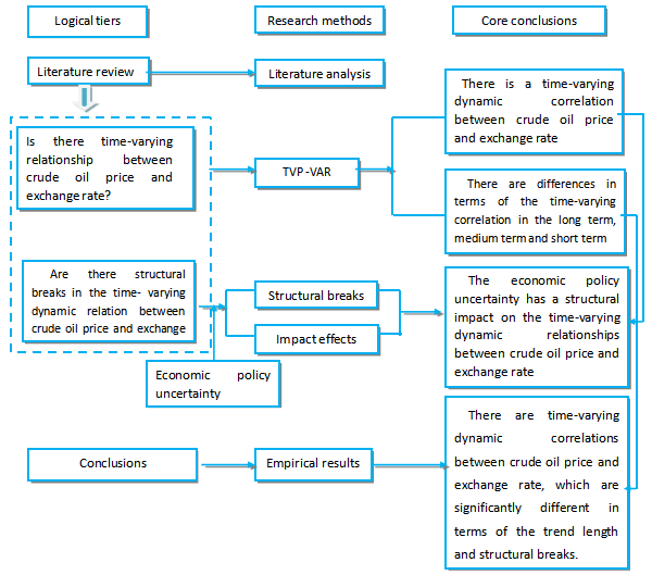
3. Analysis of Time-Varying Characteristics of Crude Oil Price and Exchange Rate Fluctuation

3.1. Parameter Estimation

There is a specific process in the parameter estimation of TVP-VAR, and the estimation method of this model is relatively mature, so it is not introduced in detail here. The paper of J Nakajima [53] can be referred to for details. Based on the original data and using the setting model (4), this paper sets the initial value of parameters according to experience, simulates 50,000 times with the MCMC algorithm and obtains effective samples, and then we get the parameter estimation results as shown in

Table 2. Estimation results of selected parameters in the TVP-VAR model.

Parameter	Mean	Std.Dev	95% L 1	95% U 2	Geweke 3	Inef. 4
${\left({\sum }_{\beta }\right)}_1$	0.0224	0.0025	0.0182	0.0278	0.419	12.13
${\left({\sum }_{\beta }\right)}_2$	0.0218	0.0024	0.0177	0.0271	0.938	15.74
${\left({\sum }_a\right)}_1$	0.0741	0.0249	0.0414	0.1371	0.806	99.22
${\left({\sum }_a\right)}_2$	0.0436	0.0079	0.0311	0.0619	0.109	36.37
${\left({\sum }_h\right)}_1$	0.3372	0.0812	0.2002	0.5162	0.589	68.95
${\left({\sum }_h\right)}_2$	0.4130	0.0823	0.2668	0.5880	0.780	54.50

Notes: 1. 95% lower credible interval limit; 2. 95% upper credible interval limit; 3. Geweke convergence diagnostics statistics; 4. Inefficiency.

.

Table 2 displays the estimation results of selected parameters in the TVP-VAR model of oil prices, U.S. REER and policy uncertainty computed with the MCMC algorithm, including posterior mean, posterior standard deviation, 95% confidence interval, Geweke’s CD convergence diagnosis value and invalid influence factors. In terms of convergence, the Geweke values of the parameters do not exceed 1.96, which is the 5% critical value. There is no evidence to reject $H_0$ of the Geweke convergence test for each parameter, where $H_0$ of the Geweke convergence diagnostics test is that the posterior distribution is convergent. It can be seen from Table 2 that the Inef. value of each parameter is far less than 50,000 sampling times, and the maximum value is about 99. This means that at least 505 (50000/99) unrelated samples can be obtained under the condition of 50,000 consecutive samples. Therefore, the number of samples obtained by the above method is sufficient for the posterior inference of the TVP-VAR model.

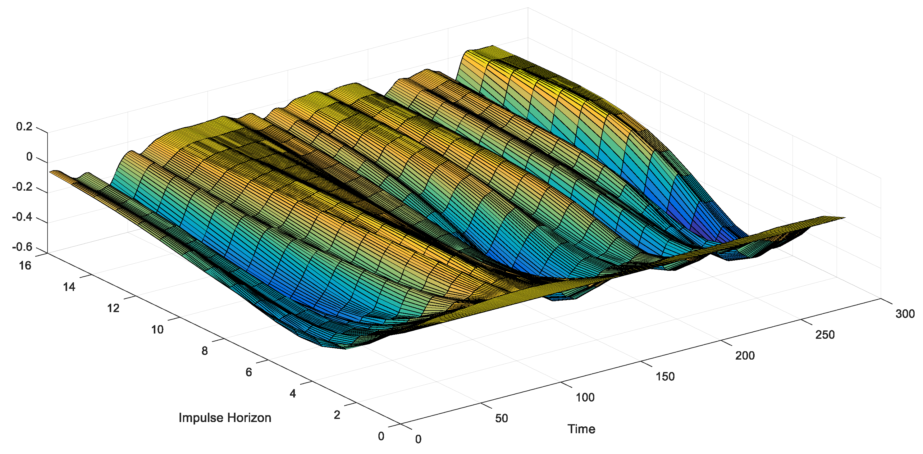
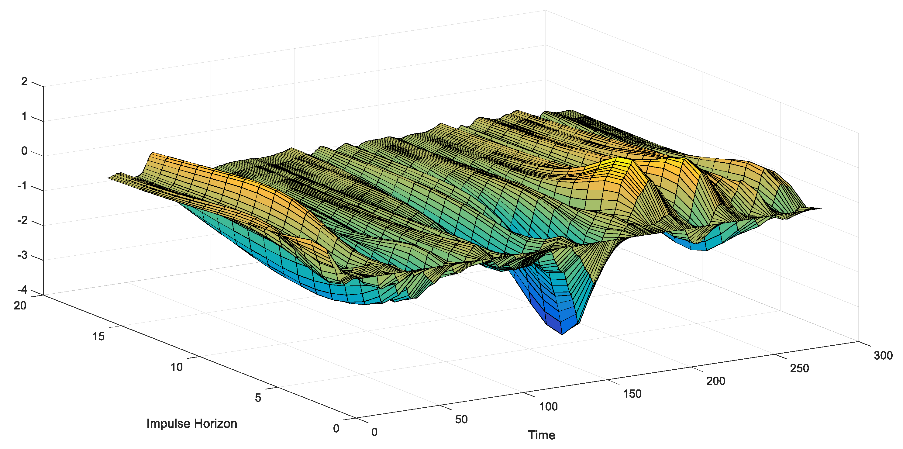
3.2. The Time-Varying Characteristics of the Correlation between Crude Oil Price and Exchange Rate Fluctuations

Further using the established model (4), the time-varying characteristics of the correlation between crude oil price and exchange rate fluctuations can be obtained, as shown in Figure 1. The simultaneous relation of the oil price and the U.S. exchange rate ($e\to er$) almost remains fluctuating below zero, and the frequency is in the middle of the three simultaneous relations presented in Figure 1. Conversely, the simultaneous relation of the oil price to the economic policy uncertainty ($e\to epu$) varies over time, showing a trend of slow decline.

The correlation between crude oil price and exchange rate is time varying. According to the estimation results of the TVP-VAR model (as shown in Figure 1), the parameters of the action of crude oil price on the exchange rate fluctuate between −0.25 and 0, while the parameters of the action of the exchange rate on the price of crude oil fluctuate between −0.25 and 0.5, showing the time-varying correlation between the two.

As for the simultaneous relation of the economic policy uncertainty to exchange rate ($epu\to er$), it fluctuates around zero violently. The estimation results of simultaneous relations suggest that there exist different forms of volatility transmission in three kinds of simultaneous relations, which means further tests are necessary.

3.3. Analysis of Time-Varying Characteristics of the Correlation between Crude Oil Price and Exchange Rate Fluctuation with Time-Delay

Section 3.2 simply describes the dynamic relationship between crude oil price and exchange rate. However, the relationship between crude oil price and exchange rate fluctuation has a time lag in the impact. This discrepancy is mainly reflected in two aspects: on the one hand, the impact of crude oil price on the exchange rate needs certain channels. When the crude oil price changes, various participants in the financial market will make decisions through their own judgment, so the exchange rate fluctuations caused by the crude oil price fluctuations will reveal after the decision of investors, and this decision-making process will produce time lag [54,55,56]. On the other hand, it takes time to digest information such as the causes of crude price fluctuations. When the price of financial assets fluctuates in the market, there is a lot of noise in the market, and the understanding of the noise will become more adequate over time. Therefore, the correlation between crude oil price and exchange rate fluctuation not only has a time lag, but the time-delay has a different length. Based on this, the dynamic relation with time-delay is studied in this paper. The impulse responses are plotted in the form of time series, showing the size of the impulses for 3-period, 6-period and 12-period horizons over time. The results are shown in Figure 2.

The impulse responses of the exchange rate to a positive oil price shock (${\epsilon }_e\to er$) vary significantly around zero over time. From 1996 to 2004, the impulse responses remain negative, and they turn to fluctuate around zero from 2004 to 2007. In the final phase of the sample period, more negative impulse responses are observed. In general, we observe much more negative impulse responses than positive impulse responses throughout the whole sample period, which means that oil prices exert negative impacts on the U.S. exchange rate movements for most of the time. During the global financial crisis, the influence of economic factors, supply and demand of crude oil and other factors on oil price shifted to exchange rate fluctuations, resulting in an obvious abnormal dynamic relationship between oil prices and exchange rate fluctuations in the short term. In the long run, the dynamic relationship between the two shows a significantly negative trend.

The impulse responses of the exchange rate to a positive economic policy uncertainty shock (${\epsilon }_{epu}\to er$) are estimated to be frequent fluctuation without an obvious pattern. From 1996 to 1999, the impulse responses are mostly below 0, and from 1999 to 2000 they increase rapidly. Since 2000, the impulse responses have been fluctuating near zero with higher frequency. From the perspective of world economic trends, the dynamic impact of uncertain economic trends on exchange rate fluctuations is consistent with the economic trends of major developed and emerging economies, changes in geopolitical relations, and changes in oil supply and demand [57,58]. Therefore, when hit by a positive shock from the economic policy uncertainty, the exchange rates fluctuate violently around zero.

The impulse responses of the economic policy uncertainty to a positive oil price shock (${\epsilon }_e\to epu$) stay negative mostly over the period from 1996 to 2019. Before 2002, the impulse responses remain fluctuating negatively, and there is a rapid upward trend from 2002 to 2004. In 2004, they return to negative volatility and have since remained below zero.

Through the above analysis, it is found that the impact of crude oil price on exchange rate is basically negative in the short, medium and long term, but the response degrees are different. Figure 2 depicts the spillover effects among variables in the short term, medium term and long term. After the impact of crude oil price, the exchange rate changes show negative responses in most of the time, and the response degree is larger in the short term and smaller in the long term. The economic policy uncertainty affects the spillover effect between them.

4. Time-Varying Characteristics of Crude Oil Price and Exchange Rate Based on Structural Breaks

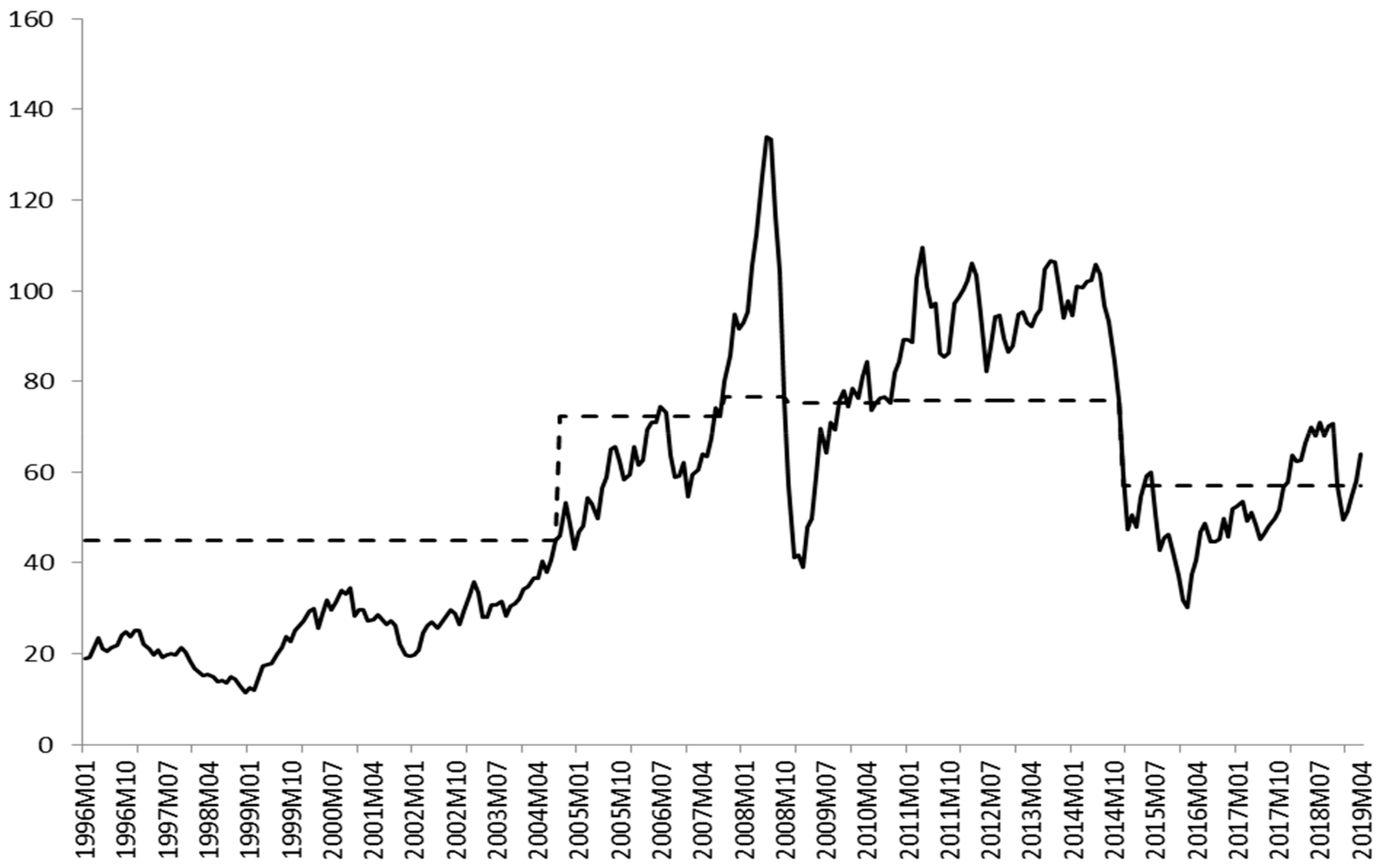
4.1. Unit Root Test in the Presence of Structural Breaks

As the price of crude oil is subject to many complex factors, there may be leaps or breaks in crude oil price fluctuation. The structural breaks obtained by existing literature are inconsistent, but all of them prove that there are breaks in crude oil price fluctuation. Nusair and Olson [59] found that the crude oil market has structural breaks and the impact of such structural breaks on other financial assets has significant asymmetric effects. Meanwhile, there is a certain “regime switch mechanism” in the price fluctuation of crude oil markets. Under different regimes, the impact of crude oil price on exchange rate is significantly different. In order to preliminarily determine whether there are breaks in the fluctuation of crude oil price, the crude oil price during the sample period is plotted as a graph, as shown in Figure 3.

As can be seen from Figure 3, there are certain breaks in the crude oil price during the sample period. It is worth noting that a lot of literature requires the hypothesis of whether there is a structural break to test the breaks. When we test the breaks of crude oil price, it is not clear whether there is a structural break. Therefore, based on Bai and Perron [60,61], we conduct the structural break tests, and

Table 3. Results of structural break tests.

Specifications
$Z_t=\left\{1\right\}$	$q=1$	$p=0$	$h=28$	$M=6$
Tests 1
$Sup{F}_T\left(1\right)$	$Sup{F}_T\left(2\right)$	$Sup{F}_T\left(3\right)$	$Sup{F}_T\left(4\right)$	$Sup{F}_T\left(5\right)$	$Sup{F}_T\left(6\right)$	$UD\max$
1.313	2.336	4.524	19.578	50.672	60.303	60.303
$SupF\left(2\left|1\right.\right)$	$SupF\left(3\left|2\right.\right)$	$SupF\left(4\left|3\right.\right)$	$SupF\left(5\left|4\right.\right)$	$SupF\left(6\left|5\right.\right)$		$MD\max$
3.783	1.773	3.459	3.458	0.663		60.303
Number of breaks selected 2
Sequential		BIC		LWZ
5		5		4
Estimates with Five Breaks 3
$SE\left(1\right)$	$SE\left(2\right)$	$SE\left(3\right)$	$SE\left(4\right)$	$SE\left(5\right)$	$SE\left(6\right)$
1.606 (0.565)	1.443 (0.620)	1.841 (1.396)	1.701 (3.551)	1.572 (1.066)	1.496 (1.346)
$T\left(1\right)$	$T\left(2\right)$	$T\left(3\right)$	$T\left(4\right)$	$T\left(5\right)$
2004M8	2007M8	2008M10	2010M9	2014M11
(03M11-05M7)	(07M6-08M4)	(06M12-09M3)	(10M7-13M2)	(13M11-15M1)

Notes: 1. The $Sup{F}_T\left(k\right)$ tests and the reported standard errors and confidence intervals allow for the possibility of serial correlation in the disturbances. The heteroscedasticity and autocorrelation consistent covariance matrix is constructed following Andrews and Monahan [62] using a quadratic kernel with automatic bandwidth selection based on an AR(1) approximation. The residuals are pre-whitened using a VAR (1). 2. We use a 5% size for the sequential test $SupF\left(k+1\left|k\right.\right)$. 3. Those in parentheses are the standard errors (robust to serial correlation) for $SE\left(i\right)\left(i=1,\dots ,6\right)$ and the 95% confidence intervals for $T\left(i\right)\left(i=1,\dots ,5\right)$.

reports the results of testing multiple breaks in oil price movements from January 1996 to April 2019. This method can effectively identify multiple breaks when the number is unknown.

As shown in Table 3, the breaks dates are estimated at 2004M8, 2007M8, 2008M10, 2010M9 and 2014M11. In general, since the 95% confidence intervals cover only a few quarters before and after the breaks dates, the five structural breaks are estimated. Among them, the fourth date, at the 95% significance level, has a rather large confidence interval between 2010M7 and 2013M2. The five breaks dates coincide with the growth in oil demand in 2004 caused by the economic development of emerging economies; the global financial crisis in 2008 triggered by the subprime crisis in the United States in 2007; the recovery of the global economy, industrialization of emerging economies, and rising geopolitical tensions in 2010 [63]; the economic slowdown of Eurozone, Japan and emerging economies; and the glut of crude oil in 2014. Therefore, there were three “rising shocks”, which occurred in 2004M8, 2007M8, and 2010M9, and two “falling shocks” which occurred in 2008M10 and 2014M11. In summary, the results of structural break tests are generally consistent with major changes affecting the trend of international oil prices, including fluctuations in economic factors, geopolitical factors, supply and demand, and climate factors on the whole. Figure 3 shows a series of oil prices with five structural breaks.

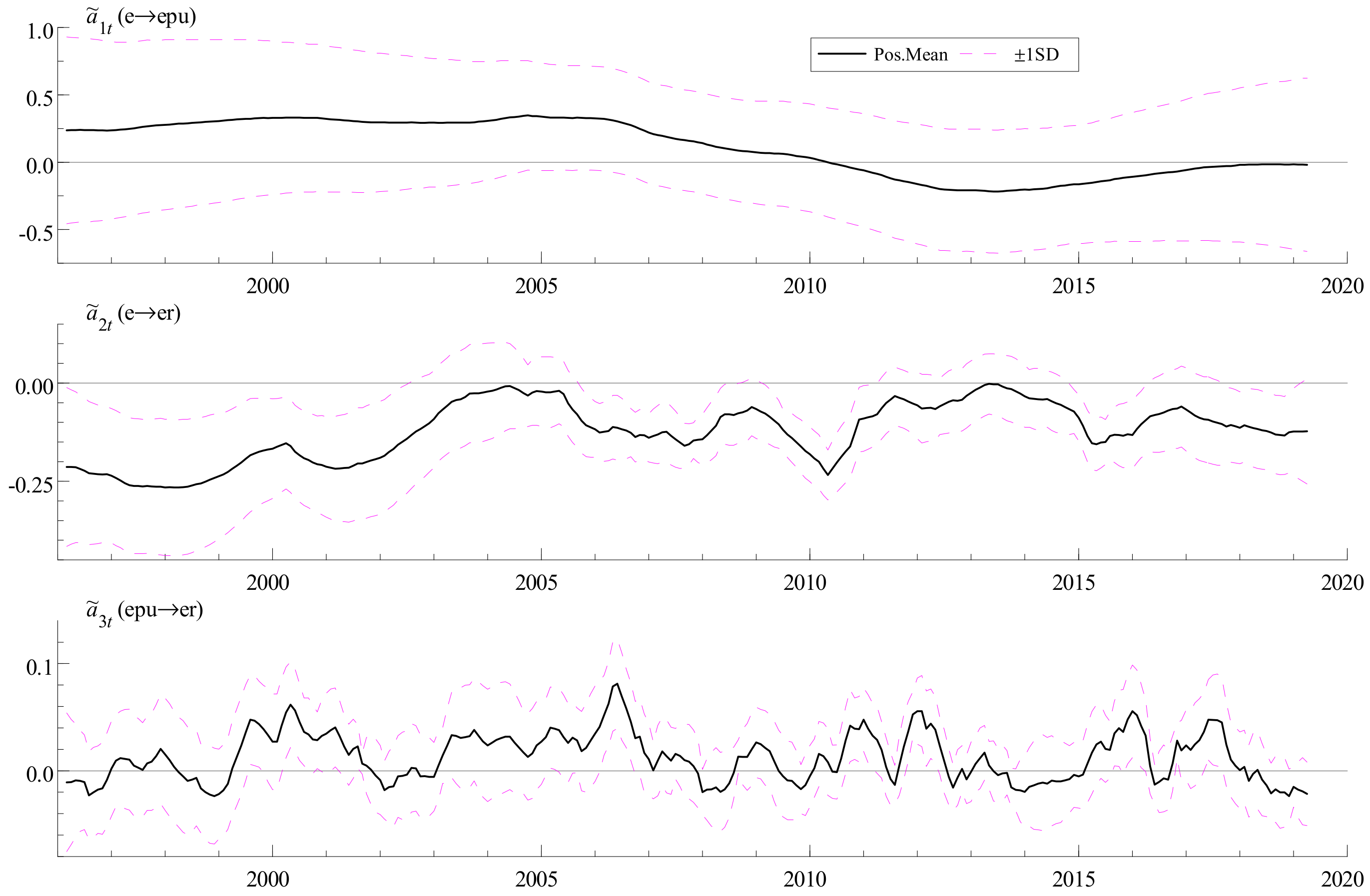
4.2. Estimation of Impulse Response Function Based on Structural Breaks

Five structural breaks dates are identified in Section 4.1, and impulse responses for the TVP-VAR model are computed to analyze the impact of time-point shocks on different variables. It is worth noticing that the date of November 2018 seems like a potential structural break date, but it doesn’t pass the structural break test due to the data limitation. Hereon, we introduce this potential structural breaks date to examine the time-point shocks of oil prices on exchange rate movements. The results are shown in Figure 4 and Figure 5.

As shown in Figure 4 and Figure 5, the impulse responses of the exchange rate to a positive oil price shock (${\epsilon }_e\to er$) rise rapidly after only one period in August 2004 and remain positive growth after four periods. A similar trend can be observed in November 2018. The impulse responses increase slowly after one-period fall and stay negative mostly in the 14 periods in October 2008, September 2010 and November 2014. Besides, the impulse response keeps negative and close to zero with significant fluctuations in August 2007. Since 2004M8, 2007M8, and 2010M9 are rising breaks, while 2008M10, 2014M11 and 2018M11 are falling breaks, there is no evidence to classify the impact of rising oil price shocks on exchange rate movements and the impact of falling oil price shocks on exchange rate movements.

Similarly, the impulse responses of the exchange rate to a positive economic policy uncertainty shock (${\epsilon }_{epu}\to er$) converge to zero in about 10 periods aftershocks with different trends for six structural breaks. In terms of the impulse responses of the economic policy uncertainty to a positive oil price shock (${\epsilon }_e\to epu$), the trends for six structural breaks are similar, which decline at the first time and increase rapidly in 2-period, converging to zero in 10-period.

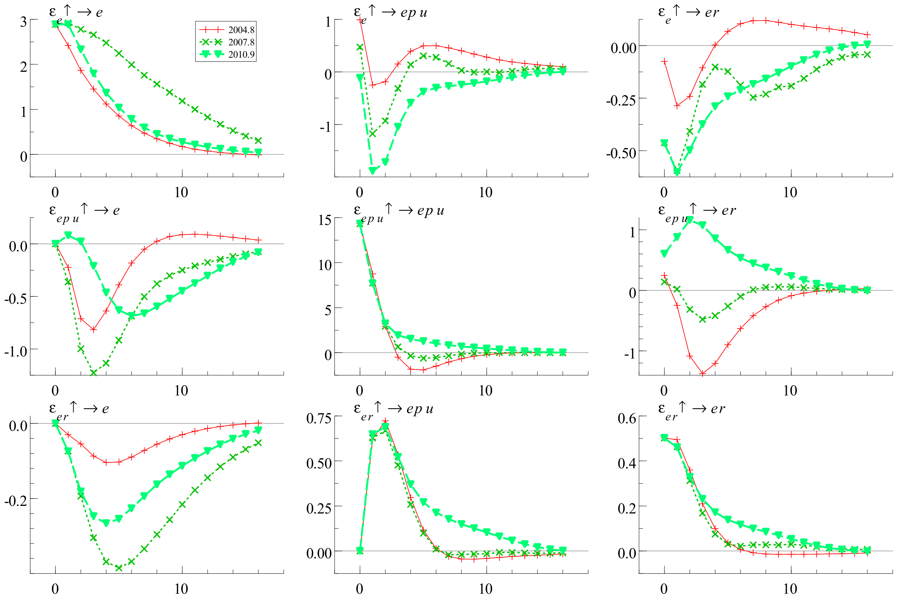
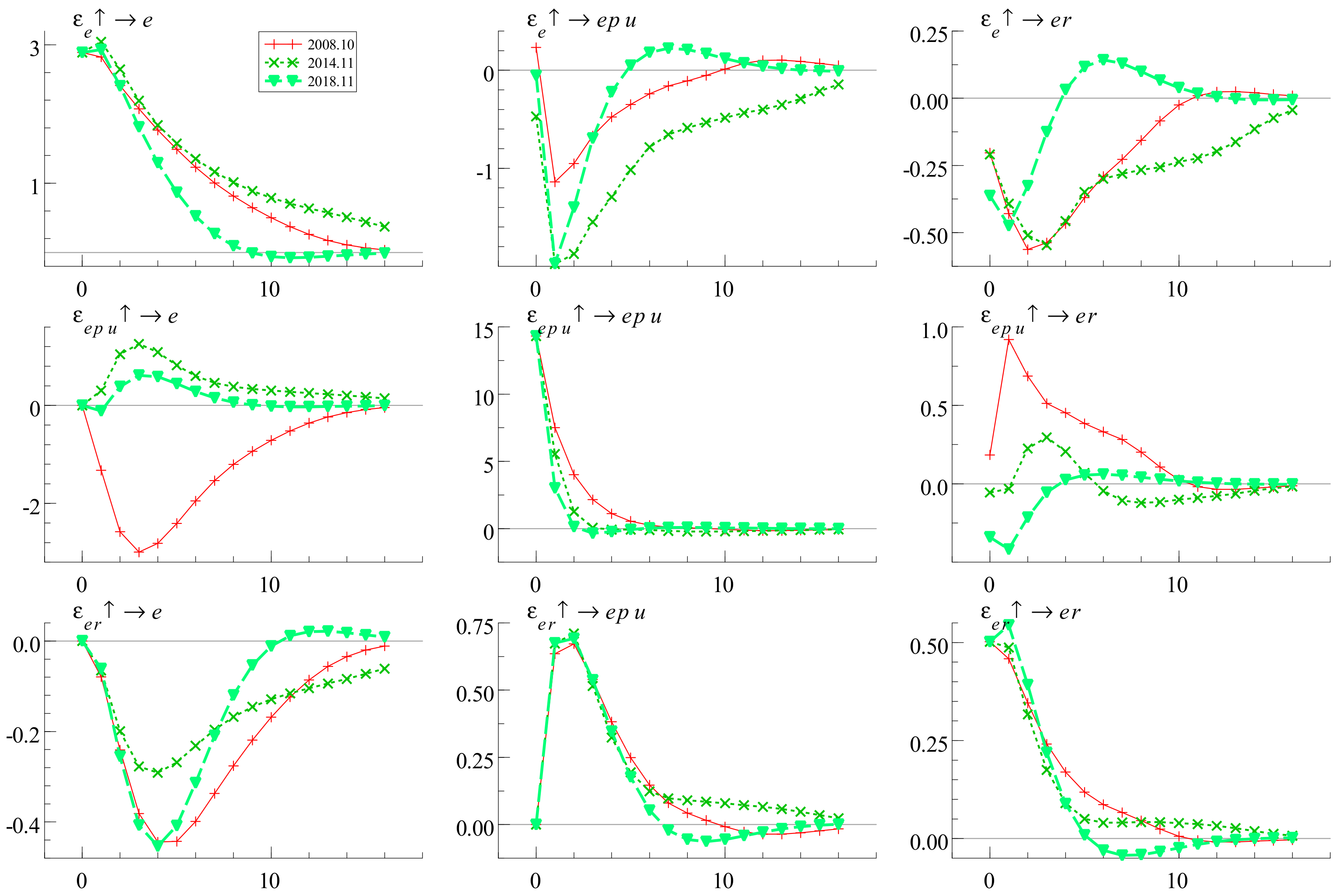
4.3. Time-Varying Characteristics Based on Structural Breaks

Since the oil price has a break structure, the oil price will change correspondingly to the exchange rate shock, and the dynamic correlation between oil price and exchange rate will change accordingly. In general, the point of time at which dynamic changes are most likely to occur is near the breakpoint. Figure 6 shows the dynamic relationship between oil price and exchange rate when oil price break impact occurs.

As shown in Figure 6, the evolution of the exchange rate due to a change in oil price is estimated for a horizon of 16 months and for each moment over the period from March 1996 to April 2019. The exchange rate is expected to decline immediately after the positive impact of oil prices. After one to four periods of shocks, the exchange rate rose then fluctuated slightly. For time intervals close to six structural breaks, the impulse responses experience fluctuations with peaks and valleys. The direct reason is that the U.S. dollar has been the dominant currency of the oil market, therefore a hike of oil prices is inclined to strengthen the U.S. dollar as members of the Organization of the Petroleum Exporting (OPEC) prefer to hold U.S. dollars [64]. Yousefi and Wirjanto [65] found that most OPEC countries adjusted the value of crude oil prices to the U.S. dollar to ensure market share and purchasing power of oil revenues. A 10% depreciation of the U.S. dollar would cause a 1.9%–8.5% rise in crude oil prices in U.S. dollars. Conversely, rising of oil prices suggests depreciation of the U.S. dollar. The decline of U.S. REER indicates the purchasing power of the U.S. dollar in foreign countries is relatively decreasing. The deeper reason is based on the theory of equilibrium exchange rates, in which movements in the real exchange rate are closely related to the Balassa-Samuelson effect, the net foreign assets and the terms of trade [65,66,67]. Soaring oil prices would affect trade balances of all countries. In the late 1990s, the U.S. is a major oil importer in the world, and as one of the petroleum importers, it has to depreciate its currency to handle its deteriorated trade balances [11]. Thanks to technological advancement and capital assistance, the United States has ranked first in the world in terms of natural gas production and crude oil production in recent years (the crude oil has fluctuated slightly, and the production of the U.S. is very close to the production of Saudi Arabia and Russia), which makes it a major exporter of natural gas and crude oil. As oil prices rise, oil exporter, such as the U.S., tends to hold more external assets, leading to the appreciation in the U.S. dollar. By contrast, petroleum importers have to depreciate their currencies to handle their deteriorated trade balances [11]. Obviously, economic theories cannot give enough explanations to our empirical results. Therefore, we further analyze time-varying shocks of the oil prices on the economic policy uncertainty.

In order to further analyze the causes of the dynamic relationship between crude oil price and exchange rate after the structural breaks, the above-mentioned economic policy uncertainty is introduced, and the dynamic change relationship between various variables is shown in Figure 7.

Figure 7 depicts the evolution of the economic policy uncertainty due to changes in oil prices, which is estimated for a horizon of 16 months and for each moment over the period from March 1996 to April 2019. The economic policy uncertainty reduced immediately after a shock in oil prices. In the late 1990s and the early 2000s, the economic policy uncertainty recovered slowly from a trough and converged to zero after 10-period shocks. During the global financial crisis, the economic policy uncertainty took longer to recover from oil price shocks. After 2008, the impulse responses of the economic policy uncertainty to a positive oil price shock kept fluctuating around zero. There is evidence to support that a rise in economic policy uncertainty reduces the oil price by a statistically significant amount in a window between 12 and 16 months [68]. Accordingly, there is a negative correlation between economic policy uncertainty and oil price movements, which is supported by our study.

5. Conclusions and Policy Implications

This paper studies the dynamic relationship between crude oil price and exchange rate and draws the following conclusions.

First, the correlation between crude oil price and exchange rate is time-varying and dynamic. According to the estimation based on the TVP-VAR model, the parameters of the impact of crude oil price on the exchange rate fluctuate between −0.25 and 0, while the parameters of the impact of the exchange rate on the price of crude oil fluctuate between −0.25 and 0.5, showing time-varying correlation between the two.

Second, the impact of crude oil prices on the exchange rate is basically negative in the short term, medium term and long term, but the response degrees are different. The TVP-VAR model presents equal time interval impulse response functions in 3-period, 6-period and 12-period, which respectively describe the spillover effects among variables in the short term, medium term, and long term. After the shock of crude oil prices, the change of the exchange rate shows negative response most of the time, and the response degree is relatively large in the short term and relatively small in the long run. The economic policy uncertainty may affect the spillover effect between the two.

Third, the impact of crude oil price on the exchange rate varies greatly at different time points, and as a whole, it is negative. The TVP-VAR model presents the impulse response functions at different time points. Although they all show a trend of first decreasing, then rising and then stabilizing, the degrees are different at each time point, especially at the structural breakpoint.

Given the recent economic trend and the characteristics of relatively strong dollar, low oil price and volatility in the current oil market, our research provides first-hand evidence for the dynamic relationship between oil price and exchange rate changes under the influence of economic policy uncertainty. In the first and second quarters of 2019, due to the uncertainty of the economic situation and trade frictions between China and the United States, oil inventories in the United States increased, the manufacturing sector in the United States contracted, and the rise of international oil prices was somewhat restrained. With the changes in oil prices, the U.S. dollar either depreciates or appreciates. When oil prices remain stable at a low level, oil-exporters may be confronted with great challenges brought by low oil prices and strong U.S. dollar. In other words, how oil exporters can boost growth while keeping inflation and exchange rates stable is a tricky and complex question. As for the U.S., a unique oil exporter, low oil prices have a negative impact on its oil exports, but a strong dollar helps to offset the negative impact on its trade account. On the other hand, high oil prices promote the terms of trade of oil exporting countries and weaken the international competitiveness of oil importing countries. Oil importers, especially some emerging economies, are under enormous pressure to maintain economic stability. The uncertainty of economic policy also brings a lot of uncertainty to the adjustment of monetary policy in oil importing countries.

References

1. Wen, F.H.; Xu, L.H.; Ouyang, G.D.; Kou, G. Retail investor attention and stock price crash risk: Evidence from China. Int. Rev. Financ. Anal. 2019, 65, 15. [Google Scholar] [CrossRef]
2. Chen, H.T.; Liu, L.; Wang, Y.D.; Zhu, Y.M. Oil price shocks and US dollar exchange rates. Energy 2016, 112, 1036–1048. [Google Scholar] [CrossRef] [Green Version]
3. Chang, H.F.; Huang, L.C.; Chin, M.C. Interactive relationships between crude oil prices, gold prices, and the NT-US dollar exchange rate-a Taiwan study. Energy Policy 2013, 63, 441–448. [Google Scholar] [CrossRef]
4. Hussain, M.; Zebende, G.F.; Bashir, U.; Ding, D.H. Oil price and exchange rate co-movements in Asian countries: Detrended cross-correlation approach. Phys. A 2017, 465, 338–346. [Google Scholar] [CrossRef]
5. Cong, R.G.; Wei, Y.M.; Jiao, J.L.; Fan, Y. Relationships between oil price shocks and stock market: An empirical analysis from China. Energy Policy 2008, 36, 3544–3553. [Google Scholar] [CrossRef]
6. Jawadi, F.; Louhichi, W.; Ben Ameur, H.; Cheffou, A.I. On oil-us exchange rate volatility relationships: An intraday analysis. Econ. Model. 2016, 59, 329–334. [Google Scholar] [CrossRef]
7. Volkov, N.I.; Yuhn, K.H. Oil price shocks and exchange rate movements. Glob. Financ. J. 2016, 31, 18–30. [Google Scholar] [CrossRef]
8. Turhan, M.I.; Sensoy, A.; Hacihasanoglu, E. A comparative analysis of the dynamic relationship between oil prices and exchange rates. J. Int. Financ. Mark. Inst. Money 2014, 32, 397–414. [Google Scholar] [CrossRef]
9. Mensah, L.; Obi, P.; Bopkin, G. Cointegration test of oil price and us dollar exchange rates for some oil dependent economies. Res. Int. Bus. Financ. 2017, 42, 304–311. [Google Scholar] [CrossRef]
10. Sun, X.; Lu, X.; Yue, G.; Li, J. Cross-correlations between the US monetary policy, US dollar index and crude oil market. Phys. A Stat. Mech. Its Appl. 2017, 467, 326–344. [Google Scholar] [CrossRef]
11. Coudert, V.; Mignon, V. Reassessing the empirical relationship between the oil price and the dollar. Energy Policy 2016, 95, 147–157. [Google Scholar] [CrossRef] [Green Version]
12. Kumar, S. Asymmetric impact of oil prices on exchange rate and stock prices. Q. Rev. Econ. Financ. 2019, 72, 41–51. [Google Scholar] [CrossRef]
13. Bahmani-Oskooee, M.; Saha, S. On the effects of policy uncertainty on stock prices: An asymmetric analysis. Quant. Financ. Econ. 2019, 3, 412–424. [Google Scholar] [CrossRef]
14. Basher, S.A.; Haug, A.A.; Sadorsky, P. Oil prices, exchange rates and emerging stock markets. Energy Econ. 2012, 34, 227–240. [Google Scholar] [CrossRef] [Green Version]
15. Bildirici, M.E.; Badur, M.M. The effects of oil prices on confidence and stock return in China, India and Russia. Quant. Financ. Econ. 2018, 2, 884–903. [Google Scholar] [CrossRef]
16. Jones, C.M.; Kaul, G. Oil and the stock markets. J. Financ. 1996, 51, 463–491. [Google Scholar] [CrossRef]
17. Sornette, D.; Cauwels, P.; Smilyanov, G. Can we use volatility to diagnose financial bubbles? Lessons from 40 historical bubbles. Quant. Financ. Econ. 2018, 2, 1–105. [Google Scholar] [CrossRef]
18. McLeod, R.C.D.; Haughton, A.Y. The value of the US dollar and its impact on oil prices: Evidence from a non-linear asymmetric cointegration approach. Energy Econ. 2018, 70, 61–69. [Google Scholar] [CrossRef]
19. Anoruo, E. Testing for Linear and Nonlinear Causality between Crude Oil Price Changes and Stock Market Returns. Int. J. Econ. Sci. Appl. Res. 2012, 4, 75–92. [Google Scholar]
20. De Vita, G.; Trachanas, E. ‘Nonlinear causality between crude oil price and exchange rate: A comparative study of China and India’—A failed replication (negative type 1 and type 2). Energy Econ. 2016, 56, 150–160. [Google Scholar] [CrossRef]
21. Ewing, B.T.; Malik, F. Modelling asymmetric volatility in oil prices under structural breaks. Energy Econ. 2017, 63, 227–233. [Google Scholar] [CrossRef]
22. Chen, L.; Du, Z.; Hu, Z. Impact of economic policy uncertainty on exchange rate volatility of China. Financ. Res. Lett. 2020, 32, 101266. [Google Scholar] [CrossRef]
23. Yang, L.; Cai, X.J.; Hamori, S. Does the crude oil price influence the exchange rates of oil-importing and oil-exporting countries differently? A wavelet coherence analysis. Int. Rev. Econ. Financ. 2017, 49, 536–547. [Google Scholar] [CrossRef]
24. Tiwari, A.K.; Albulescu, C.T. Oil price and exchange rate in India: Fresh evidence from continuous wavelet approach and asymmetric, multi-horizon Granger-causality tests. Appl. Energy 2016, 179, 272–283. [Google Scholar] [CrossRef]
25. Bartsch, Z. Economic policy uncertainty and dollar-pound exchange rate return volatility. J. Int. Money Finan. 2019, 98, 17. [Google Scholar] [CrossRef]
26. Li, Z.; Zhong, J. Impact of economic policy uncertainty shocks on China’s financial conditions. Financ. Res. Lett. 2019, 101303. [Google Scholar] [CrossRef]
27. Li, Z.H.; Dong, H.; Huang, Z.H.; Failler, P. Asymmetric effects on risks of virtual financial assets (VFAs) in different regimes: A case of bitcoin. Quant. Financ. Econ. 2018, 2, 860–883. [Google Scholar] [CrossRef]
28. Apergis, N.; Miller, S.M. Do structural oil-market shocks affect stock prices? Energy Econ. 2009, 31, 569–575. [Google Scholar] [CrossRef] [Green Version]
29. Salisu, A.A.; Fasanya, I.O. Modelling oil price volatility with structural breaks. Energy Policy 2013, 52, 554–562. [Google Scholar] [CrossRef]
30. Sadorsky, P. Modelling and forecasting petroleum futures volatility. Energy Econ. 2006, 28, 467–488. [Google Scholar] [CrossRef]
31. Kang, S.; Yoon, S. Forecasting Volatility of Crude Oil Markets. Energy Econ. 2009, 31, 119–125. [Google Scholar] [CrossRef]
32. Jian, J.; Gu, R. Asymmetrical long-run dependence between oil price and US dollar exchange rate—Based on structural oil shocks. Phys. A Stat. Mech. Its Appl. 2016, 456, 75–89. [Google Scholar] [CrossRef]
33. Bai, D.P.; Rath, B.N. Nonlinear causality between crude oil price and exchange rate: A comparative study of China and India. Energy Econ. 2015, 51, 149–156. [Google Scholar] [CrossRef]
34. Mollick, A.V.; Sakaki, H. Exchange rates, oil prices and world stock returns. Resour. Policy 2019, 61, 585–602. [Google Scholar] [CrossRef]
35. Jain, A.; Biswal, P.C. Dynamic linkages among oil price, gold price, exchange rate, and stock market in India. Resour. Policy 2016, 49, 179–185. [Google Scholar] [CrossRef]
36. Reboredo, J.C. Modelling oil price and exchange rate co-movements. J. Policy Model. 2012, 34, 419–440. [Google Scholar] [CrossRef]
37. Ji, Q.; Shahzad, S.J.H.; Bouri, E.; Suleman, M.T. Dynamic Structural Impacts of Oil Shocks on Exchange Rates: Lessons to Learn; Springer: Berlin/Heidelberg, Germany, 2020; Volume 9. [Google Scholar] [CrossRef] [Green Version]
38. Brémond, V.; Hache, E.; Razafindrabe, T. On the link between oil price and exchange rate: A time-varying VAR parameter approach. Work. Pap. 2015. [Google Scholar] [CrossRef]
39. Wen, F.; Xiao, J.; Huang, C.; Xia, X. Interaction between oil and US dollar exchange rate: Nonlinear causality, time-varying influence and structural breaks in volatility. Appl. Econ. 2018, 50. [Google Scholar] [CrossRef]
40. Castro, C.; Jiménez-Rodríguez, R. Time-Varying Relationship between Oil Price and Exchange Rate. MPRA Paper. 2018. Available online: https://mpra.ub.uni-muenchen.de/87879/ (accessed on 9 October 2019).
41. Primiceri, G.E. Time varying structural vector autoregressions and monetary policy. Rev. Econ. Stud. 2005, 72, 821–852. [Google Scholar] [CrossRef]
42. Jebabli, I.; Arouri, M.; Teulon, F. On the effects of world stock market and oil price shocks on food prices: An empirical investigation based on tvp-var models with stochastic volatility. Energy Econ. 2014, 45, 66–98. [Google Scholar] [CrossRef]
43. Liao, G.K.; Li, Z.H.; Du, Z.Q.; Liu, Y. The heterogeneous interconnections between supply or demand side and oil risks. Energies 2019, 12, 17. [Google Scholar] [CrossRef] [Green Version]
44. Xu, Y.; Han, L.; Wan, L.; Yin, L. Dynamic link between oil prices and exchange rates: A non-linear approach. Energy Econ. 2019, 84. [Google Scholar] [CrossRef]
45. Balcilar, M.; Gupta, R.; Kyei, C.; Wohar, M.E. Does economic policy uncertainty predict exchange rate returns and volatility? Evidence from a nonparametric causality-in-quantiles test. Open Econ. Rev. 2016, 27, 229–250. [Google Scholar] [CrossRef] [Green Version]
46. You, W.; Guo, Y.; Zhu, H.; Tang, Y. Oil price shocks, economic policy uncertainty and industry stock returns in China: Asymmetric effects with quantile regression. Energy Econ. 2017, 68, 1–18. [Google Scholar] [CrossRef]
47. Dong, H.; Liu, Y.; Chang, J. The heterogeneous linkage of economic policy uncertainty and oil return risks. Green Financ. 2019, 1, 46–66. [Google Scholar] [CrossRef]
48. Beckmann, J.; Czudaj, R.L.; Arora, V. The relationship between oil prices and exchange rates: Revisiting theory and evidence. Energy Econ. 2020. [Google Scholar] [CrossRef]
49. Baker, S.R.; Bloom, N.; Davis, S.J. Measuring Economic Policy Uncertainty. Chicago Booth Research Paper No. 13-02; SSRN. 2013. Available online: https://ssrn.com/abstract=2198490 (accessed on 9 October 2019). [CrossRef] [Green Version]
50. Baker, S.R.; Bloom, N.; Davis, S.J. Measuring economic policy uncertainty. Q. J. Econ. 2016, 131, 1593–1636. [Google Scholar] [CrossRef]
51. Jarque, C.M.; Bera, A.K. Efficient tests for normality, homoscedasticity and serial independence of regression residuals. Econ. Lett. 1980, 6, 255–259. [Google Scholar] [CrossRef]
52. Hodrick, R.J.; Prescott, E.C. Postwar US business cycles: An empirical investigation. J. Money Credit Bank. 1997, 24, 1–16. [Google Scholar] [CrossRef]
53. Nakajima, J. Time-Varying Parameter VAR Model with Stochastic Volatility: An Overview of Methodology and Empirical Applications. Available online: https://www.imes.boj.or.jp/research/papers/english/11-E-09.pdf (accessed on 9 October 2019).
54. Brahmasrene, T.; Huang, J.C.; Sissoko, Y. Crude oil prices and exchange rates: Causality, variance decomposition and impulse response. Energy Econ. 2014, 44, 407–412. [Google Scholar] [CrossRef]
55. Kido, Y. On the link between the US economic policy uncertainty and exchange rates. Econ. Lett. 2016, 144, 49–52. [Google Scholar] [CrossRef]
56. Troster, V.; Shahbaz, M.; Uddin, G.S. Renewable energy, oil prices, and economic activity: A Granger-causality in quantiles analysis. Energy Econ. 2018, 70, 440–452. [Google Scholar] [CrossRef] [Green Version]
57. Huang, Z.H.; Liao, G.K.; Li, Z.H. Loaning scale and government subsidy for promoting green innovation. Technol. Forecast. Soc. Chang. 2019, 144, 148–156. [Google Scholar] [CrossRef]
58. Li, Z.H.; Liao, G.K.; Wang, Z.Z.; Huang, Z.H. Green loan and subsidy for promoting clean production innovation. J. Clean Prod. 2018, 187, 421–431. [Google Scholar] [CrossRef]
59. Nusair, S.A.; Olson, D. The effects of oil price shocks on Asian exchange rates: Evidence from quantile regression analysis. Energy Econ. 2019, 78, 44–63. [Google Scholar] [CrossRef]
60. Bai, J.S.; Perron, P. Estimating and testing linear models with multiple structural changes. Econometrica 1998, 66, 47–78. [Google Scholar] [CrossRef]
61. Bai, J.; Perron, P. Computation and analysis of multiple structural change models. J. Appl. Econom. 2003, 18, 1–22. [Google Scholar] [CrossRef] [Green Version]
62. Andrews, D.W.K.; Monahan, J.C. An improved heteroskedasticity and autocorrelation consistent Covariance-matrix estimator. Econometrica 1992, 60, 953–966. [Google Scholar] [CrossRef]
63. Li, Z.; Liao, G.; Albitar, K. Does corporate environmental responsibility engagement affect firm value? The mediating role of corporate innovation. Bus. Strateg. Environ. 2019. [Google Scholar] [CrossRef]
64. Golub, S.S. Oil prices and exchange-rates. Econ. J. 1983, 93, 576–593. [Google Scholar] [CrossRef]
65. Yousefi, A.; Wirjanto, T.S. Exchange rate of the US dollar and the j curve: The case of oil exporting countries. Energy Econ. 2003, 25, 741–765. [Google Scholar] [CrossRef]
66. Coudert, V.; Couharde, C.; Mignon, V. Does Euro or dollar pegging impact the real exchange rate? The case of oil and commodity currencies. World Econ. 2011, 34, 1557–1592. [Google Scholar] [CrossRef]
67. Wen, F.H.; Zhao, Y.P.; Zhang, M.Z.; Hu, C.Y. Forecasting realized volatility of crude oil futures with equity market uncertainty. Appl. Econ. 2019, 51, 6411–6427. [Google Scholar] [CrossRef]
68. Kang, W.S.; Ratti, R.A. Oil shocks, policy uncertainty and stock market return. J. Int. Financ. Mark. Inst. Money 2013, 26, 305–318. [Google Scholar] [CrossRef]
Figure 1. Posterior estimates for simultaneous relations.
Energies 13 02395 g001
Figure 2. Time-varying impulse responses of the TVP-VAR model.
Energies 13 02395 g002
Figure 3. WTI crude oil prices in 1996M1–2019M4.
Energies 13 02395 g003
Figure 4. Time-varying impulse responses of the TVP-VAR model for structural breaks. Notes: 1. Horizontal axes indicate the number of months after a shock. 2. Vertical axes represent the standardized responses to shocks for each variable.
Energies 13 02395 g004
Figure 5. Time-varying impulse responses of the TVP-VAR model for structural breaks (continued). Notes: 1. Horizontal axes indicate the number of months after a shock. 2. Vertical axes represent the standardized responses to shocks for each variable.
Energies 13 02395 g005
Figure 6. Impulse response function of the exchange rate due to a change in the level of the oil price, for 16 months and in each moment from 1996M3 up until 2019M4 (Time axis).
Energies 13 02395 g006
Figure 7. Impulse response function of the economic policy uncertainty due to a change in the level of the oil price for 16 months and in each moment in time from 1996M3 up until 2019M4 (Time axis).
Energies 13 02395 g007