Article

A Sliding Mode Control Strategy with Repetitive Sliding Surface for Shunt Active Power Filter with an LCLCL Filter

1
College of Electronics and Information Engineering, Taiyuan University of Science & Technology, Taiyuan 030024, China
2
State Grid Taiyuan Power Supply Company, Taiyuan 030024, China
3
College of Electrical and Power Engineering, Taiyuan University of Technology, Taiyuan 030024, China
*
Author to whom correspondence should be addressed.
Energies 2020, 13(7), 1740; https://doi.org/10.3390/en13071740
Submission received: 4 March 2020 / Revised: 3 April 2020 / Accepted: 3 April 2020 / Published: 5 April 2020
(This article belongs to the Special Issue Control Strategies for Power Conversion Systems)

Abstract

:
This paper proposes a novel sliding mode control (SMC) scheme with a repetitive sliding surface for shunt active power filters (SAPF) to enhance the system robustness and eliminate harmonic current tracking errors. Traditional control schemes, such as PI control, repetitive control (RC), proportional resonance control (PR), improve the stability of the SAPF in the stable grid to a certain extent. However, the robustness of the SAPF control system has not been improved. In this paper, the SMC is applied to SAPF, and a sliding mode controller is constructed by using a linear sliding mode surface composed of the system state variables and a fast exponential power-reaching law, which can effectively enhance the system robustness. When the grid parameters change or external disturbances exist, sliding surface drift and sliding mode chattering will occur. Although fast-tracking of the harmonic current can still be achieved, it is difficult to accurately compensate AC harmonic current. Moreover, this may cause the harmonic current compensation error to be amplified. RC can achieve infinite gain at multiples of the fundamental frequency and can track inputs without static errors. In order to fully eliminate the harmonic current tracking error and effectively suppress the total harmonic distortion (THD) of the grid, the sliding mode surface was modified. An RC term of harmonic current error is introduced to the sliding mode surface, and a novel plugin-repetitive sliding mode control strategy (RCSMC) for SAPF is proposed. Finally, simulation and experiment results on the LCLCL-filter based SAPF show the effectiveness of the proposed control strategy.

Graphical Abstract

1. Introduction

Traditional control schemes applied to shunt active power filters (SAPF), such as PI control, repetitive control (RC), proportional resonance control (PR), and their hybrid control, can compensate the current harmonics accurately in the stable power grid [1,2,3]. This meets the expected requirements of industrial occasions. However, when the power grid parameters fluctuate, the transfer function of the SAPF control system is changed, which will cause system instability and affect system robustness. The sliding mode control (SMC) strategy has been applied in SAPF due to its good dynamic response, strong robustness, and good regulation performance in a wide operating condition. Various SMC methods for SAPF have been proposed [4,5]. Their robustness is always enhanced, and the steady-state accuracy is also highlighted.
In practical applications, the SMC method is implemented by a digital system. It needs to detect intermediate variables using multiple sensors, construct a state equation, and then establish the sliding mode surface. To meet the desired control objectives, it also relies on high switching frequency to achieve the sliding mode surface reach and follow. The ideal SMC method requires infinite switching of the power switches, so that the system state should always meet the sliding mode, ensuring the sliding mode motion, realizing accurate tracking, zero error adjustment and fast dynamic response [6,7]. However, during the SMC implementation, chattering caused by non-ideal infinite switch switching, discrete system delay, unmodeled dynamic effects and parameter uncertainty will restrict the steady-state compensation accuracy of the control system [8]. In the current research, the steady-state performance of SMC is improved by reaching law design and sliding surface modification. In general, the common linear sliding surface is composed of a linear combination of system state variables. When the system parameters are changed or external interference exists, the sliding surface would drift, which will affect the system output tracking error. Integral sliding mode control (ISMC), and intelligent SMC incorporating fuzzy logic and artificial neural networks have become a research focus, to improve SMC performance [8,9,10,11]. In [12], the integral term of the state variables is introduced into the sliding mode-switching function in the SMC to eliminate the steady-state error. In [13,14], an ISMC method is proposed for DC-DC converters and DC-AC inverters, which uses sequential integration to smooth chatter and improve system steady-state accuracy. Based on ISMC, a new dual-integral sliding mode controller (DISMC) is present for the maximum power point tracker (MPPT) in DC tracking systems [15]. The double integration term of tracking voltage error was used in its sliding surface to eliminate steady-state errors. Z. Liu [16] proposed a new sliding mode surface based on the learning rate, which maintains the advantages of high sliding speed of the traditional SMC strategy. The convergence speed will become slower when the error variable approaches the sliding mode surface, so the chattering problem that is caused by the high convergence speed can be suppressed and the system tracking accuracy can be improved. However, for AC tracking systems, these methods can reduce steady-state errors, but they cannot fully reduce the sinusoidal tracking errors of the inverter [13]. For SAPF, the above methods have a limited tracking ability for harmonics, and ISMC is prone to problems such as large overshoot and long adjustment time, which deteriorate transient performance. To address these deficiencies, [17] introduced a multi-resonance term of grid-connected current error on the sliding mode surface, and a multiresonance sliding mode controller (MRSMC) is proposed, which eliminated the grid-connected current tracking error by using the high-loop gain characteristics of resonance control to the periodic signal. The derivation and demonstration are only for a single-phase grid-connected inverter, and the influence of grid fluctuations on resonance control is not fully considered.
In this paper, a sliding mode controller composed of a linear sliding mode surface of state variables and a fast exponential power reaching law is designed to enhance the robustness of the SAPF. Furtherly, aiming at the steady-state error problem caused by chattering and parameter uncertainty, the sliding mode surface was modified. Considering the advantages of RC with gain amplification for harmonics and non-static error tracking for periodic signals, an RC term of harmonic current error is introduced to the sliding mode surface, and a novel plugin-repetitive sliding mode control strategy (RCSMC) for SAPF is proposed. Finally, simulation and experiment results on the LCLCL-based SAPF show the effectiveness of the proposed control strategy.
The rest of this paper is organized as follows: in Section 2, the SMC for SAPF with an LCLCL filter is designed. In Section 3, the RCSMC is proposed. An RC term of harmonic current error is introduced to the sliding mode surface to suppress the tracking error and THD. Section 4 and Section 5 present the simulation and experimental results, respectively. Finally, conclusions are stated in Section 6.

2. Sliding Mode Control Model Analysis

2.1. Sliding Mode Controller Design

Figure 1 shows the control system of the SAPF with an LCLCL filter. The main topology consists of a voltage source inverter and an LCLCL filter. The inverter is a harmonic generator. The DC side capacitors Cd1 and Cd2 are used to keep the DC voltage udc constant. The LCLCL filter is used to filter out the SAPF output current ripple. Where, Ls is the grid equivalent inductor, L1 is grid side inductor, L2 is inverter side inductor, Cf is filter capacitor, and Rd is parasitic damping resistor of Cf. The system introduces a resonant branch consisting of Lh and Ch, which is tuned at the switching frequency of the inverter. As a bandpass filter for switching ripple, it also reduces the power loss of the damping resistor. The non-linear load is a three-phase diode rectifier with a resistive load. In Figure 1, udc is the dc bus voltage; us is the grid voltage; ui is the inverter output voltage; uc is the capacitor branch voltage, and is, iL, ish, ic, iinv is grid current, current drawn by the non-linear load, SAPF grid-connected current, capacitor current, and inverter output current, respectively. The main circuit parameters are shown in Table 1.
The harmonic current control scheme is given in the control circuit part of Figure 1. It can be seen that the harmonic command current is calculated by detecting the load current and using the d-q method based on the instantaneous reactive power theory. The composite current controller is used to control the inverter to provide a compensated harmonic current for the non-linear load. As a result, the grid current becomes an ideal sine wave. The inverter DC-side bus voltage is modulated by the traditional PI control strategy, which provides active power during harmonic compensation.
The voltage and current vectors in Figure 1 are defined as follows
i i n v = [ i i n v a i i n v b i i n v c ] , i s h = [ i s h a i s h b i s h c ] , u i = [ u i a u i b u i c ] , u c = [ u c a u c b u c c ] , u s = [ u s a u s b u s c ]
The secondary parasitic series resistor associated with the inductor in the main circuit can be ignored in modeling, control design and simulation [18,19]. Because the additional LhCh resonant branch has an operating bandwidth that exceeds the Nyquist frequency, the controller design is not affected even if LhCh is ignored. Therefore, SAPF control model can be denoted as
{ L 2 d i i n v d t = u i u c C f d u c d t = i i n v i s h L 1 d i s h d t = u c u s
The inverter output voltage vector u i in (1) can be expressed as follows, according to its relationship to the DC-side voltage udc:
u i = [ u i a u i b u i c ] = s k u d c = [ s a u d c 2 s b u d c 2 s c u d c 2 ]
where sk is the switching state. It can be defined as
s k = { 1 When   the   upper   arm   is   turned   on   and   the   lower   arm   is   turned   off 0 When   the   upper   arm   is   turned   off   and   the   lower   arm   is   turned   on   ( k = a , b , c )
To further simplify the analysis, when the frequency is high enough, the high-frequency component of the PWM wave is ignored, and the PWM duty cycle dk (the average value of sk in one switching cycle) is used to replace sk [20]. Then, (2) can be written as
u i = [ u i a u i b u i c ] = d k u d c = [ d a u d c 2 d b u d c 2 d c u d c 2 ]
Therefore, the continuous-time dynamic model can be expressed as
{ L 2 d i i n v d t = d k u d c 2 u c C f d u c d t = i i n v i s h L 1 d i s h d t = u c u s
For a three-phase symmetrical system, the three phases can be controlled independently. The analysis is based on the A- phase. The dynamic model of the A-phase can be written as
{ L 2 d i i n v a d t = d a u d c 2 u c a C f d u c a d t = i i n v a i s h a L 1 d i s h a d t = u c a u s a
where each symbol is a physical quantity of the A-phase. da is the duty cycle of A-phase, which is the control input of the A- phase. The sliding mode controller is designed based on the A-phase system model. The other two phases are similar to the A-phase, and the derivation results are consistent.
Define state variables x1a, x2a and x3a as
x 1 a = i i n v a i i n v a ,   x 2 a = u c a u c a ,   x 3 a = i s h a i s h a
where i i n v a , u c a and i s h a is the A-phase reference for inverter output current, the reference for filter capacitor voltage, and the reference for the SAPF grid-connected current (that is, harmonic command current), respectively. Those satisfy (5), and i i n v a and u c a can be written as
u c a = L 1 i ˙ s h a + u s a
i i n v a = C f u ˙ c a + i s h a
x1a, x2a and x3a are the three error variables concerned. If the three error variables tend to 0 through the control input da, SAPF can achieve perfect harmonic compensation. Construct a state space equation as follows
X ˙ = A X + B u + D
where, X ˙ = [ x ˙ 1 a x ˙ 2 a x ˙ 3 a ] T , X = [ x 1 a x 2 a x 3 a ] T , u is the control law.
From (5) to (8), the following can be derived (assuming the grid voltage is constant):
x ˙ 1 a = i ˙ i n v a i ˙ i n v a = d a u d c 2 L 2 u c a L 2 i ˙ i n v a = d a u d c 2 L 2 x 2 a L 2 u c a L 2 i ˙ i n v a
x ˙ 2 a = u ˙ c a u ˙ c a = i i n v a C f i s h a C f ( i i n v a C f i s h a C f ) = 1 C f x 1 a 1 C f x 3 a
x ˙ 3 a = i ˙ s h a i ˙ s h a = u c a u s a L 1 u c a u s a L 1 = x 2 a L 1
Then, the coefficients and state inputs of the system state space equation can be described as
A = [ 0 1 L 2 0 1 C f 0 1 C f 0 1 L 1 0 ] ,   B = [ u d c 2 L 2 0 0 0 0 0 0 0 0 ] ,   D = [ u c a L 2 i ˙ i n v a 0 0 ] ,   u = [ d a 0 0 ]
Select linear sliding mode switching function σa can be described as
σ a = C X = [ α 1 α 2 α 3 ] X
where α1, α2 and α3 are positive real constants for achieving system stability.
The sliding mode motion suffers from the chattering, which may cause current harmonic misalignment and affect the accuracy of harmonic compensation. Therefore, in order to improve the quality of sliding mode motion and effectively suppress high-frequency chattering, a fast exponential power reaching law is selected [21]. The reaching law meets the reaching condition and makes the system stable.
σ ˙ a = k 1 σ a k 2 | σ a | γ sgn ( σ a ) k 1 > 0 , k 2 > 0 , 0 < γ < 1
Substituting (9), (13), and (14) into (15), (15) can be rewritten as
σ ˙ a = C X ˙ = C A X + C B u + C D = k 1 σ a k 2 | σ a | γ sgn ( σ a )
By solving (16), the control law u of the system can be obtained, and the duty cycle da can be obtained as
d a = 2 u d c [ α 2 L 2 α 1 C f ( x 1 a x 3 a ) ( α 3 L 2 α 1 L 1 1 ) x 2 a + ( u c a + L 2 i ˙ i n v a ) ] + 2 L 2 α 1 u d c ( k 1 σ a k 2 | σ a | γ sgn ( σ a ) )
where,
  • d a _ e q = 2 u d c [ α 2 L 2 α 1 C f ( x 1 a x 3 a ) ( α 3 L 2 α 1 L 1 1 ) x 2 a + ( u c a + L 2 i ˙ i n v a ) ]
    d a _ l = k 1 2 L 2 α 1 u d c σ a
    d a _ n = k 2 2 L 2 α 1 u d c | σ a | γ sgn ( σ a )
From (17), the control input da can be divided into three parts: an equivalent part da_eq, a linear part da_l, and a non-linear part da_n. Where the equivalent part da_eq is an equivalent control law that can be obtained by solving σ ˙ a = 0 , the linear part da_l and the non-linear part da_n are compensation effects of the fast exponential power-reaching law. Therefore, the A-phase control block diagram of SAPF based on SMC can be shown in Figure 2, where, the inverter output gain KPWM is udc/2. The control law of B-phase and C-phase is the same as that of the A-phase.

2.2. Error Analysis of Sliding Mode Controller

From (11) and (12), it can be obtained as follows
x 2 a = L 1 x ˙ 3 a
x 1 a = C f x ˙ 2 a + x 3 a = C f L 1 x ¨ 3 a + x 3 a
Therefore, the sliding mode switching function becomes
σ a = α 1 x 1 a + α 2 x 2 a + α 3 x 3 a = α 1 C f L 1 x ¨ 3 a + α 2 L 1 x ˙ 3 a + ( α 1 + α 3 ) x 3 a
It can be seen that the sliding mode switching function is still essentially a linear combination of harmonic current tracking error and its various derivatives. Then, the sliding mode surface σ a = 0 can be deduced as
x ¨ 3 a + α 2 α 1 C f x ˙ 3 a + ( α 1 + α 3 ) α 1 C f L 1 x 3 a = 0
Assuming m = α 2 α 1 C f , n = ( α 1 + α 3 ) α 1 C f L 1 , then
x ¨ 3 a + m x ˙ 3 a + n x 3 a = 0
The harmonic current error x3a can be obtained as
x 3 a = C 1 e ( m 2 + 1 2 m 2 4 n ) t + C 2 e ( m 2 1 2 m 2 4 n ) t
Obviously, as long as m > 0 and n > 0 are guaranteed, the compensation current error x3a will tend to 0 when the steady state is reached, but an infinite switching frequency is required to achieve a high-precision steady-state performance. From (17), the control input da is closely related to the system parameters. Renewable energy is often produced far from the power load center and transmitted through long transmission lines and a large number of transformers, which causes the grid impedance to increase. In addition, temperature, voltage, and harmonics also affect the value of the capacitor. As a result, the system parameters will appear uncertain. In fact, because the system modeling is not necessarily accurate, and the system modeling may also be affected by the changes in system parameters or external interference, the sliding surface will drift, which will increase the output tracking error of the system. From (17) and (23), the harmonic current error x3a is directly related to the grid-connected inductor L1 and the filter capacitor Cf, and is related to the inverter-side inductor L2 through the control input da. The change in the parameters will directly affect the result of x3a. Taking the uncertainty of the filter capacitor Cf and the grid-side inductance L1 as examples, they are analyzed as follows.
Assuming that the initial nominal values of the filter capacitor and the grid-side inductor are Cf and L1, respectively, and those variations are ΔCf and ΔL1, the actual values after the change can be expressed as
C f = C f + Δ C f ,   L 1 = L 1 + Δ L 1
After the filter parameters change, the reference value of the filter capacitor voltage u c a and the reference value of the inverter-side inductor current i i n v a also change accordingly. The reference value of the grid-connected inductor current i s h a is given by the calculation of the harmonic detection algorithm, which is only related to the load and not affected by parameter changes. Therefore, (7) and (8) should be written as
u c a = L 1 i ˙ s h a + u s a = L 1 i ˙ s h a + u s a + Δ L 1 i ˙ s h a = u c a + Δ L 1 i ˙ s h a
i i n v a = C f u ˙ c a + i s h a = C f u ˙ c a + Δ C f u ˙ c a + i s h a = i i n v a + C f Δ L 1 i ¨ s h a + Δ C f u ˙ c a + Δ C f Δ L 1 i ¨ s h a
Consequently, the state variables x1a and x2a can be written as
x 1 a = i i n v a i i n v a = x 1 a C f Δ L 1 i ¨ s h a Δ C f u ˙ c a Δ C f Δ L 1 i ¨ s h a
x 2 a = u c a u c a = u c a u c a Δ L 1 i ˙ s h a = x 2 a Δ L 1 i ˙ s h a
Therefore, the sliding mode switching function can be modified as
σ a = α 1 x 1 a + α 2 x 2 a + α 3 x 3 a = α 1 x 1 a + α 2 x 2 a + α 3 x 3 a Δ σ a
where
Δ σ a = α 1 C f Δ L 1 i ¨ s h a + α 1 Δ C f u ˙ c a + α 1 Δ C f Δ L 1 i ¨ s h a + α 2 Δ L 1 i ˙ s h a
From (29), because of the inaccurate system modeling, the actual sliding surface is drifted by Δσ.
The harmonic current reference and grid voltage are set as
i s h a = k = 1 n o I s h k sin ( k ω t )
u s a = U s a sin ( ω t )
Then, the sliding surface offset can be written as
Δ σ a = α 1 ( C f + Δ C ) Δ L 1 ω 2 k = 1 n o k 2 I s h k sin ( k ω t ) α 1 Δ C f ( ω 2 L 1 k = 1 n o k 2 I s h k sin ( k ω t ) + ω U s a cos ( ω t ) ) + α 2 Δ L 1 ω k = 1 n o k I s h k cos ( k ω t )
From (20), σ a can be rewritten as
σ a = α 1 C f L 1 x ¨ 3 a + α 2 L 1 x ˙ 3 a + ( α 1 + α 3 ) x 3 a Δ σ a
The sliding surface can be modified as
x ¨ 3 a + m x ˙ 3 a + n x 3 a + h 1 k = 1 n o k 2 I s h k sin ( k ω t ) + h 2 k = 1 n o k I s h k cos ( k ω t ) + h 3 cos ( ω t ) = 0
where
  • m = α 2 α 1 C f , n = ( α 1 + α 3 ) α 1 C f L 1 ,
    h 1 = ω 2 ( C f + Δ C f ) Δ L 1 + ω 2 L 1 Δ C f C f L 1 , h 2 = α 2 Δ L 1 ω α 1 C f L 1 , h 3 = ω Δ C f U s a C f L 1 .
Compared with (22), the AC tracking error is introduced into the sliding surface, and the error term x3a can be calculated by the dsolve function in MATLAB. In addition to the first two items in (23), there are many harmonic components in the calculation results. Obviously, the defects in the system model make the sliding surface drift, which increase the harmonic current tracking error, and seriously affect the grid current THD.

3. Plug-in Repetitive Sliding Mode Controller Design

According to the internal model principle, the system controller can realize a zero tracking error control only if it contains the mathematical model which can generate the required reference input. RC is based on the internal model principle. It is able to provide an infinite loop gain for all harmonics. According to the nature of the exponential function [22], the internal model structural form of RC in the time domain can be expressed as
G R C ( s ) = k R C × e s T 1 e s T = k R C 2 + k R C T s + 2 k R C T n s s 2 + n 2 ω 2
where, kRC is the RC gain, T is the fundamental period of the input signal, ω is the fundamental frequency, and n is the harmonic order.
From (35), the internal model of the RC is very similar to the typical PR control. Compared with the PR control, the RC internal model adds a proportional control term, an integral control term which has infinite gain to the DC signal, and a multi-resonance control term which has infinite gain to the AC signal at multiple fundamental frequency. Therefore, the repetitive controller is essentially a combination of the PI and multi-resonant control. In practice, in order to increase the stability margin, a filter, Q, is usually connected in series in the internal model (taken as a constant less-than-1 or a low-pass filter). When Q is constant, (35) can be written as [23]
G R C ( s ) = k R C × Q e s T 1 Q e s T k R C 2 + k R C T s + 2 k R C T n s s 2 + 2 ω c s + n 2 ω 2
where, ωc is the resonance frequency, and ω c = ln Q T . When the ωc is much smaller than ω, (36) is established.
Obviously, compared with (35), the multi-resonance term in (36) has changed, which is similar to the structure of the PR controller. Therefore, as in [17], adding a multi-PR term, it is possible to add an RC term for the harmonic current error x3a into the sliding mode switching function.
First, after performing Laplace transform on (29), the sliding mode switching function can be transformed into a sliding mode in the s domain.
σ a ( s ) = α 1 x 1 a ( s ) + α 2 x 2 a ( s ) + α 3 x 3 a ( s ) Δ σ a ( s )
where
Δ σ a ( s ) = α 1 ω 2 ( C f Δ L 1 + Δ C f Δ L 1 + Δ C f L 1 ) k = 1 n o k 2 I s h k k ω s 2 + k 2 ω 2 α 1 Δ C f ω U s a s s 2 + ω 2 + α 2 Δ L 1 ω k = 1 n o k I s h k s s 2 + k 2 ω 2
Then, introducing the RC term, the sliding mode switching function can be modified as
σ a ( s ) = α 1 x 1 a ( s ) + α 2 x 2 a ( s ) + α 3 x 3 a ( s ) + G R C ( s ) x 3 a ( s )
When the disturbance of the filter capacitor and the grid-side inductor exists, the harmonic error x3a(s) can be solved according to the sliding surface constructed by (38) after introducing an RC term
x 3 a ( s ) = h 1 k = 1 n o k 2 I s h k k ω s 2 + k 2 ω 2 + h 2 k = 1 n o k I s h k s s 2 + k 2 ω 2 + h 3 s s 2 + ω 2 s 2 + m 1 s + n 1 + G R C ( s )
where, G R C ( s ) = G R C ( s ) α 1 C f L 1 , other coefficients are consistent with the above.
To simplify the analysis, considering only the harmonic current has a 7th order harmonic portion, (39) can be rewritten as
x 3 a ( s ) = 49 h 1 I s h 7 7 ω s 2 + 49 ω 2 + 7 h 2 I s h 7 s s 2 + 49 ω 2 + h 3 s s 2 + ω 2 s 2 + m 1 s + n 1 + G R C ( s )
when △L1 = 0.1 mH, △Cf = 1 uF, Ish7=1 A, kRC = 1, ω = 100π, ωc = 20, the bode plot of x3a(s) is shown in Figure 3.
From Figure 3, the error x3a(s) has a large attenuation at the fundamental frequency and the harmonic frequency when RCSMC is applied, and the amplitude gain is less than −200 dB. Therefore, any harmonic error can be attenuated when the filter parameters are changed. Similarly, for other defects in the system model, the harmonic tracking errors can also be eliminated. It is proved that adding an RC term to the sliding surface can replace the multiple resonance term and play a better role in error correction. Obviously, the SAPF system based on RCSMC can not only enhance robustness, but also achieve full harmonic compensation and further reduce steady state errors.
The A-phase control block diagram of the SMC system with RC term is shown in Figure 4. In Figure 4, an RC term of harmonic current error x3a is introduced to the sliding mode surface. The repetitive controller transfer function GRC (s) can achieve the best harmonic compensation by reasonably adding a compensator C(z) when the discrete implementation. According to [24], the compensator C(z) is composed of three parts: proportional gain kr, phase lead zk, and filter S(z). For the system parameters in this paper, the compensator is designed as [24]:
C ( z ) = k r z k S ( z ) = 0.95 × z 5 × z 2 + 2 + z 2 4 × 0.6291 z + 0.2634 z 2 0.1922 z + 0.08476

4. Simulation Results Analysis

To verify the proposed RCSMC scheme, the SAPF model with an LCLCL-filter is built in MATLAB. Compared with the traditional SMC, MRSMC and feedforward RC methods, the steady-state simulation and dynamic-state simulation is performed, respectively. For non-linear load, the DC side resistance of the rectifier is 40 Ω. The main circuit parameters and controller parameters are shown in Table 1 and Table 2.

4.1. Steady-State Characteristics

Figure 5, Figure 6 and Figure 7 show the simulation results of the steady-state waveform and spectrum of the grid current using SMC, MRSMC and RCSMC. The THD of the grid current is 1.87%, 1.29%, 0.82%, respectively. At the same non-linear load conditions, RCSMC scheme is the best. After the RC term is introduced into the sliding mode surface, the harmonic content of the grid current is further reduced, and all orders of which are lower than 0.2%. It is evident that RCSMC scheme can attenuate all other harmonics and improve the accuracy of harmonic compensation.
Figure 8 shows the A-phase harmonic current error x3a(t) waveform using the SMC, MRSMC and RCSMC strategy. The x3a(t) waveform using traditional SMC is shown in Figure 8a. It is evident from Figure 8a that the uncertainty of system modeling and parameters make the sliding mode surface drift, which affects the harmonic current tracking error. As shown in Figure 8b, the harmonic current error x3a(t) is greatly reduced using MRSMC (the amplitude decreases from 3 A to 1 A), and the x3a(t) waveform is similar to the harmonic reference. However, the MRSMC strategy has a limited ability to achieve gain amplification for all order harmonics, so that it cannot fully eliminate the harmonic current error in steady state. The harmonic current error x3a(t) using RCSMC, as shown in Figure 8c, is further reduced. The amplitude of the harmonic current error is about 0.4 A, and the amplitude of the grid current is about 13.98 A. Compared with the other two control strategies, the high-precision compensation of the current harmonics is realized using RCSMC. Although the design of an RC internal model filter Q(z) and compensator C(z) is limited by the system stability so as to affect the harmonic compensation precision, the results presented are already excellent.

4.2. Dynamic Characteristics

Figure 9 shows the dynamic simulation waveform of the grid current using RCSMC under the non-linear load step change. The non-linear load current amplitude is changed form 13.98 A to 20.39 A in 0.63 seconds. It can be seen that, when the non-linear load step changes, SAPF has good tracking ability and grid current is has perfect sinusoidal waveform. Due to the introduction of the RC term, there is a small distortion point at the peak of the current in the transient process, but the proposed control strategy still has a good dynamic response.

4.3. Robustness Analysis

An important feature of SMC is its strong robustness, which is reflected in the insensitivity of the control system to changes in grid parameters or SAPF parameters or external disturbances. When grid parameters are changed or disturbances exist, the system should not only maintain stability but also have perfect steady-state accuracy. By changing the grid inductor Ls (0.1 to 0.5 mH), the filter parameters L1 (△L1 = 0.1 mH) and Cf (△Cf = 1 uF), the anti-disturbance capability of the SAPF is verified in feedforward RC and RCSMC at the same nonlinear load condition, respectively, as shown in Figure 10 and Figure 11.
Figure 10 shows the dynamic simulation results when the grid inductor Ls and filter parameters change in 0.53 seconds. As shown in Figure 10a, using the feedforward RC, the harmonic current error x3a increases by about ±1 A, and the grid current isa presents a distortion. The THD increased from 2.85% to 4.33%. As shown in Figure 10b, using RCSMC, the harmonic current error x3a increased by ± 0.1 A in an instant. The grid current THD changed from 0.82% to 0.94%.
Figure 11 shows the steady-state simulation results after the grid inductor Ls and filter parameters change. As can be seen from Figure 11a, using the feedforward RC, the results show that there is a significant error in the harmonic compensation current ish and the grid current is compensation accuracy decreases. The grid current is THD increased from the previous 4.33% to 8.05%, and the system becomes gradually unstable as the control model changes. As can be seen from Figure 11b using RCSMC, the reaching of the sliding mode surface has nothing to do with grid parameters, so the system is stable, and the THD remained at 0.94%, and the grid current waveform was still close to a standard sine wave. The simulation results show that, under the change in grid impedance and filter parameters, the feedforward RC strategy cannot suppress the external disturbances and make the system unstable, while the RCSMC method enables the grid to obtain precise and stable harmonic compensation and strong robustness.

5. Analysis of Experimental Results

An overview of the experimental platform built in the laboratory is shown in Figure 12. The platform consists of a 3-kVA SAPF with LCLCL filter and a 6-kVA three-phase uncontrolled rectified non-linear load with the parameters listed in Table 1 and Table 2. The total DC capacitor of SAPF is 3300 μF (Cd1 and Cd2 are respectively composed of two 3300 μF in parallel). The proposed control strategy was implemented in TMS320F28335 DSP based on experimental platform shown in Figure 1 and Figure 12.

5.1. Steady-State Experimental Results

In the steady-state experiment (the DC side is connected with 40 Ω resistor), the harmonic steady-state compensation performance is verified by using SMC, MRSMC and RCSMC. The experimental waveforms of the three control methods are shown in Figure 13, Figure 14 and Figure 15, respectively.
Figure 13 shows that the harmonic current is insufficiently compensated using SMC and the grid current is non-sinusoidal waveform with a high THD (approximately 3.4%). As described in Section 2.2 and Section 4.1, the SAPF using SMC is unable to effectively compensate the harmonic current due to imperfect system modeling and parameter uncertainty and sampling delay. The compensation current has a periodic error of about ±1 A. Figure 14 shows the grid current and harmonic error waveforms using MRSMC. It can be seen that the grid current waveform has improved significantly. In view of the sliding mode surface drift, the MRSMC exerts an influence on the sliding mode surface, so that the specified low-order harmonics are compensated. The system has high steady-state accuracy, and the grid current THD is reduced to 2.4%. The experimental waveform using RCSMC is shown in Figure 15. As can be seen, the harmonic currents are effectively compensated and the grid current is almost sinusoidal, with a small THD of about 1.7%. It is fully proved that RC can enhance the tracking ability of the periodic harmonic of SAPF system, and realize the full harmonic compensation, and further improve the steady-state accuracy by introducing a great gain at all harmonic frequencies.

5.2. Dynamic Experimental Results

To evaluate the dynamic performance with load variations, the transient responses of the SAPF using different control strategies are shown in Figure 16 and Figure 17, respectively. As shown, as soon as the load is changed from 14 to 20 A, the SAPF current quickly responds to changes to compensate harmonic current and to ensure a sine grid current. It is verified that both the MRSMC and RCSMC strategy have good dynamic responses. In comparison, because of the inherent periodic delay in the RC, the fast response of harmonics is limited, and the dynamic response speed of the RCSMC is slightly lower than that of the MRSMC. However, the reaching law and the equivalent control law can make the system state variables stabilize on the sliding mode surface in a limited time, thereby ensuring the good sliding mode motion quality. In fact, due to the effect of SMC, the response time of the grid current is minimally increased, which is far less than one period of the grid voltage. Moreover, RCSMC results in a smaller current overshoot.

5.3. Robust Experimental Result

Figure 18 shows the grid current waveform using RCSMC after the filter inductor changes. It can be seen that, after the filter inductor changes from 0.7 to 0.8 mH, the harmonic current error x3a has hardly changed. The grid current THD increased from 1.7% to 1.8%. Although the inductor changes make the system model change accordingly, which will cause the sliding mode surface to drift and AC tracking error, the sliding mode function and the fast exponential power reaching law act commonly to keep the system stable, and the introduced RC term compensates excellently the tracking error. Experimental results show that RCSMC method has strong robustness.

6. Conclusions

This paper proposes a novel sliding mode control scheme with a repetitive sliding surface for SAPF with an LCLCL filter, which effectively eliminates grid-connected harmonic current tracking errors and enhances the system robustness.
(1)
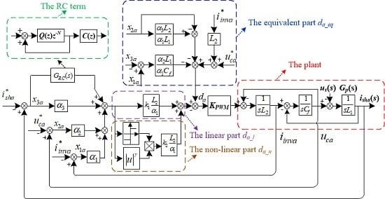
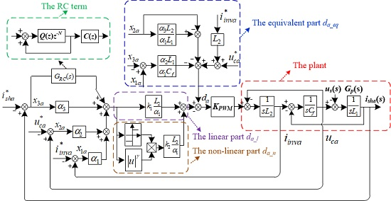
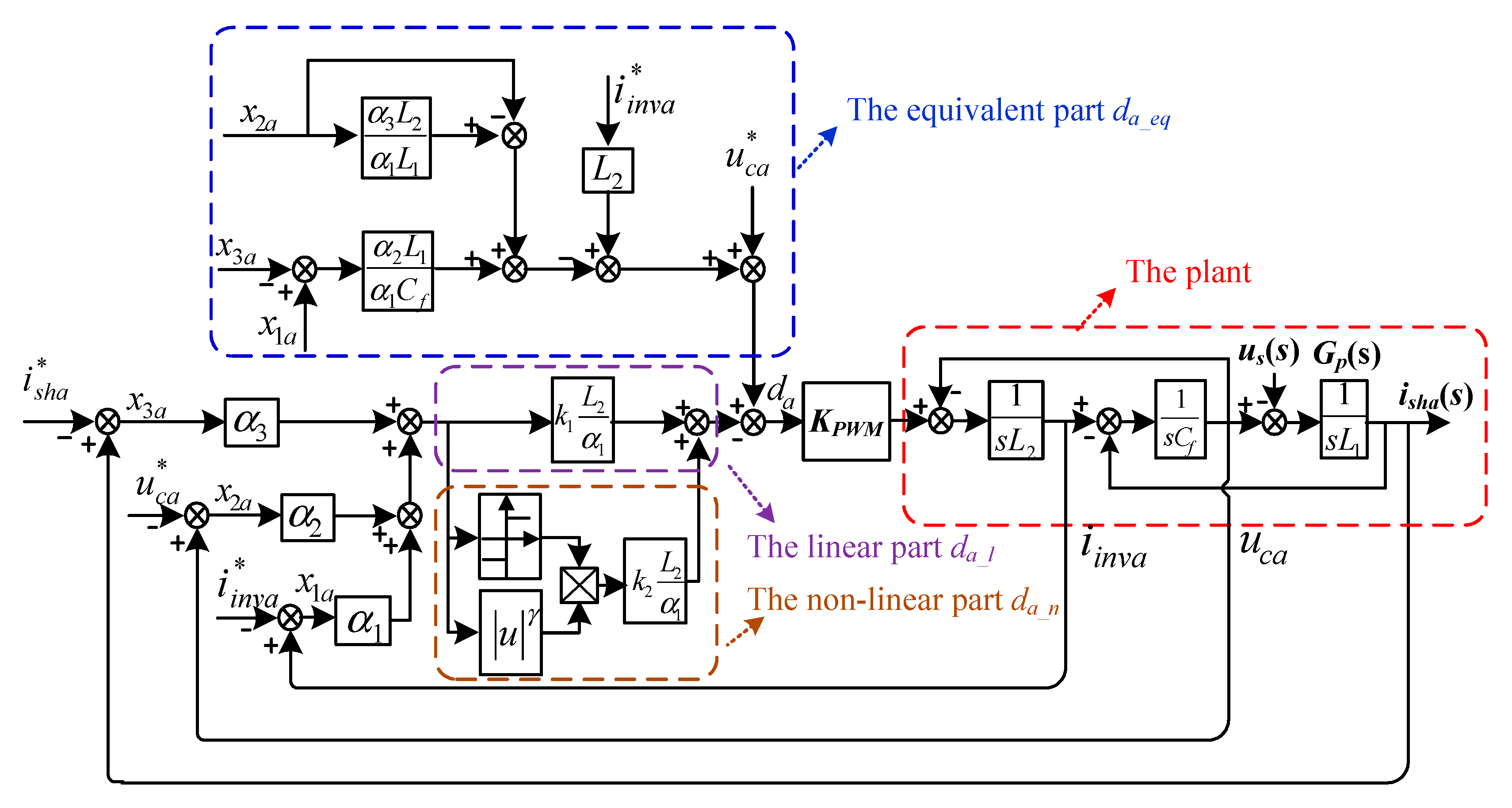
A sliding mode-switching function is established based on a linear combination of three error variables: inverter output current error, filter capacitor voltage error, and grid-connected harmonic current error. The control law is obtained through a fast exponential power reaching law. To address sliding mode surface drift caused by imperfect system modeling and system parameter uncertainty, the RC term of grid-connected harmonic current error are introduced into the sliding mode surface, and a plugin-repetitive sliding mode control strategy (RCSMC) is proposed. This strategy combines the advantages of RC and SMC to eliminate the harmonic current tracking error and suppress the grid current THD;
(2)
Simulation and experimental results on a 380 V, 3 kVA SAPF prototype show that, compared with SMC and MRSMC, the RCSMC has stronger robustness to perturbations, smaller tracking error, lower grid current THD and good dynamic response capabilities. The grid current THD can be reduced to 1.7% after compensation in experiment. The RCSMC is easier to realize in the discrete system, which has the advantage of simplicity and adaptability to SAPF.

Author Contributions

Conceptualization, Y.G. and L.Z.; methodology, Y.G.; software, Y.G. and X.L.; validation, Y.G., X.L., W.Z. and D.H.; formal analysis, L.Z.; investigation, Y.G. and D.H.; resources, Y.G.; data curation, X.L.; writing—original draft preparation, Y.G.; writing—review and editing, L.Z.; visualization, X.L.; supervision, Y.G.; project administration, D.H.; funding acquisition, Y.G. and L.Z. All authors have read and agreed to the published version of the manuscript.

Funding

This research was funded by TAIYUAN UNIVERSITY OF SCIENCE AND TECHNOLOGY SCIENTIFIC RESEARCH INITIAL FUNDING (grant number 20182047) and the Natural Science Foundation of Shanxi Province (grant number 201901D111076).

Acknowledgments

This paper and its related research work were supported by TAIYUAN UNIVERSITY OF SCIENCE AND TECHNOLOGY SCIENTIFIC RESEARCH INITIAL FUNDING (project No.20182047) and the Natural Science Foundation of Shanxi Province (project No.201901D111076).

Conflicts of Interest

The authors declare no conflict of interest.

References

  1. Lascu, C.; Asiminoaei, L.; Boldea, I.; Blaabjerg, F. Frequency response analysis of current controllers for selective harmonic compensation in active power filters. IEEE Trans. Ind. Electron. 2009, 56, 337–347. [Google Scholar] [CrossRef]
  2. Trinh, Q.; Lee, H.; Member, S. An Advanced Current Control Strategy for Three-Phase Shunt Active Power Filters. IEEE Trans. Ind. Electron. 2013, 60, 5400–5410. [Google Scholar] [CrossRef]
  3. Zeng, Z.; Yang, J.Q.; Yu, N.C. Research on PI and repetitive control strategy for Shunt Active Power Filter with LCL-filter. In Proceedings of the 7th International Power Electronics and Motion Control Conference, Harbin, China, 2–5 June 2012; pp. 2833–2837. [Google Scholar]
  4. Lu, W.; Li, C.; Xu, C. Sliding mode control of a shunt hybrid active power filter based on the inverse system method. Int. J. Electron. Power Energy Syst. 2014, 57, 39–48. [Google Scholar] [CrossRef]
  5. Alali, M.A.E.; Shtessel, Y.; Barbot, J.P. Grid-Connected Shunt Active LCL Control via Continuous Sliding Modes. IEEE Trans. Mechatron. 2019, 24, 729–740. [Google Scholar] [CrossRef]
  6. Utkin, V.I. Sliding Modes in Control and Optimization, 1st ed.; Springer: Berlin, Germany, 1992. [Google Scholar]
  7. Shtessel, Y.; Edwards, C.; Fridman, L.; Levant, A. Sliding Mode Control and Observation, 1st ed.; Birkhauser: Basel, Switzerland, 2014. [Google Scholar]
  8. Yu, X.H.; Kaynak, O. Sliding-Mode Control with Soft Computing: A Survey. IEEE Trans. Ind. Electron. 2009, 56, 3275–3285. [Google Scholar]
  9. Li, S.; Liang, X.; Fei, J. Dynamic Surface Adaptive Fuzzy Control of Three-Phase Active Power Filter. IEEE Access 2016, 4, 9451–9458. [Google Scholar]
  10. Fei, J.; Li, S. Adaptive Fractional High Order Sliding Mode Fuzzy Control of Active Power Filter. Soft Computing and Intelligent Systems (SCIS) and 19th International Symposium on Advanced Intelligent Systems (ISIS). In Proceedings of the 2018 Joint 10th International Conference, Toyama, Japan, 5–8 December 2018; pp. 576–580. [Google Scholar]
  11. Liu, N.; Fei, J. Adaptive Fractional Sliding Mode Control of Active Power Filter Based on Dual RBF Neural Networks. IEEE Access 2017, 5, 27590–27598. [Google Scholar] [CrossRef]
  12. Utkin, V.; Shi, J. Integral sliding mode in systems operating under uncertainty conditions. In Proceedings of the 35th IEEE Conference on Decision and Control, Kobe, Japan, 13 December 1996; Volume 4, pp. 4591–4596. [Google Scholar]
  13. Wai, R.J.; Wang, W.H. Grid-connected photovoltaic generation system. IEEE Trans. Circuits Syst. I Reg. Papers 2008, 55, 953–964. [Google Scholar]
  14. Levant, A. Higher-order sliding modes, differentiation and output feedback control. Int. J. Control 2003, 76, 924–941. [Google Scholar] [CrossRef]
  15. Pradhan, R.; Subudhi, B. Double Integral Sliding Mode MPPT Control of a Photovoltaic System. IEEE Trans. Control Syst. Technol. 2016, 1, 285–292. [Google Scholar] [CrossRef]
  16. Liu, Z.; Liu, X.; Cheng, J.; Fang, C. Altitude control for variable load quadrotor via learning rate based robust sliding mode controller. IEEE Access 2019, 7, 9736–9744. [Google Scholar] [CrossRef]
  17. Hao, X.; Yang, X.; Liu, T.; Huang, L.; Chen, W.A. Sliding-mode controller with multiresonant sliding surface for single-phase grid-connected VSI with an LCL filter. IEEE Trans. Power Electron. 2013, 28, 2259–2268. [Google Scholar] [CrossRef]
  18. Tang, Y.; Loh, P.C.; Wang, P.; Choo, F.H.; Gao, F. Exploring inherent damping characteristic of LCL-filters for three-phase grid-connected voltage source inverters. IEEE Trans. Power Electron. 2012, 27, 1433–1443. [Google Scholar] [CrossRef]
  19. Wang, J.; Yan, J.; Jiang, L. Pseudo-derivative-feedback current control for three-phase grid-connected inverters with LCL filters. IEEE Trans. Power Electron. 2016, 31, 3898–3912. [Google Scholar] [CrossRef] [Green Version]
  20. He, N.; Zhang, J.; Zhu, Y.; Shen, G.; Xu, D. Weighted average current control in three-phase grid inverter with LCL filter. IEEE Trans. Power Electron. 2013, 28, 2785–2797. [Google Scholar] [CrossRef]
  21. Yu, S.; Yu, X.; Shirinzadeh, B.; Man, Z. Continuous finite-time control for robotic manipulators with terminal sliding mode. Automatica 2005, 41, 1957–1964. [Google Scholar] [CrossRef]
  22. Gradshteyn, L.S.; Ryzhik, L.M. Table of Integrals, Series, and Products; Academic Press: San Diego, CA, USA, 2007; pp. 20–30. [Google Scholar]
  23. Zhu, M.Z.H.; Ye, Y.Q.; Zhao, Q. A design method of repetitive controller against variation of grid frequency. Proc. CSEE 2016, 36, 3857–3867. [Google Scholar]
  24. Gao, Y.G.; Jiang, F.Y.; Song, J.C.; Zheng, L.J.; Tian, F.Y.; Geng, P.L. A novel dual closed-loop control scheme based on repetitive control for grid-connected inverters with an LCL filter. ISA Trans. 2018, 74, 194–208. [Google Scholar] [CrossRef] [PubMed]
Figure 1. Structure of shunt active power filter (SAPF) system with an LCLCL filter.
Energies 13 01740 g001
Figure 2. A-phase control block diagram of SAPF based on sliding mode control (SMC).
Energies 13 01740 g002
Figure 3. Bode plot of harmonic error x3a(s) with plugin-repetitive sliding mode control (RCSMC).
Energies 13 01740 g003
Figure 4. A-phase control block diagram of SAPF based on RCSMC.
Energies 13 01740 g004
Figure 5. Simulation waveform of SAPF based on SMC in steady state.
Energies 13 01740 g005
Figure 6. Simulation waveform of SAPF based on multi-resonance sliding mode controller (MRSMC) in steady state.
Energies 13 01740 g006
Figure 7. Simulation waveform of SAPF based on RCSMC in steady state.
Energies 13 01740 g007
Figure 8. Waveform of x3a(t) using different control strategies.
Energies 13 01740 g008
Figure 9. Simulation waveform of SAPF based on RCSMC in dynamic state.
Energies 13 01740 g009
Figure 10. Simulation waveform of SAPF in dynamic state when the grid impedance changes.
Energies 13 01740 g010
Figure 11. Simulation waveform of SAPF in steady state when the grid impedance changes.
Energies 13 01740 g011
Figure 12. Experimental platform of SAPF with LCLCL filter.
Energies 13 01740 g012
Figure 13. Experimental waveform of the grid current and harmonic error with SMC.
Energies 13 01740 g013
Figure 14. Experimental waveform of the grid current and harmonic error with MRSMC.
Energies 13 01740 g014
Figure 15. Experimental waveform of the grid current and harmonic error with RCSMC.
Energies 13 01740 g015
Figure 16. Experimental waveform of SAPF based on MRSMC in dynamic state.
Energies 13 01740 g016
Figure 17. Experimental waveform of SAPF based on RCSMC in dynamic state.
Energies 13 01740 g017
Figure 18. Experimental waveform of SAPF based on RCSMC after the filter inductor L1 changes.
Energies 13 01740 g018
Table 1. Main parameters of SAPF system.
SymbolDescriptionValue
Ls/L1/L2/Lhinductor0.1 mH/0.7 mH/2 mH/0.3 mH
Cf/Chfilter capacitor10 uF/1 uF
Rdparasitic resistance of filter capacitor0.005 Ω
usgrid voltage380 V
udcDC bus voltage750V
fgrid voltage frequency50 Hz
fc/fscarrier frequency/sampling frequency9 kHz
Ssystem capacity3k VA
Table 2. Parameters of RCSMC.
ParametersValue
k15 × 104
k2105
γ0.3
α11
α21
α31

