Article

A Local Control Strategy for Distributed Energy Fluctuation Suppression Based on Soft Open Point

1
Institute of Electrical Engineering of the Chinese Academy of Sciences, Beijing 100190, China
2
School of Electronic, Electrical and Communication Engineering, University of Chinese Academy of Sciences, Beijing 100049, China
*
Author to whom correspondence should be addressed.
Energies 2020, 13(6), 1520; https://doi.org/10.3390/en13061520
Submission received: 17 February 2020 / Revised: 9 March 2020 / Accepted: 22 March 2020 / Published: 23 March 2020
(This article belongs to the Section C: Energy Economics and Policy)

Abstract

:
This paper proposes a local control strategy applied in the soft open point (SOP) to suppress voltage fluctuation when adding a renewable energy source into the system. The mathematic model of the grid connected to SOP is established based on the characteristics of a low-voltage distribution network. Combined with the mathematic model and local voltage information, the local control strategy is proposed to optimize the active and reactive power distribution and consume the minimum apparent power of the converter. The local control strategy can effectively suppress the voltage fluctuation caused by renewable energy access, which was testified by MATLAB/Simulink simulation. In addition, the local control strategy can deduce the communication resource and increase the response speed compared to global optimization. This paper is meaningful for renewable energy source distribution and voltage balance in low-voltage distribution systems.

1. Introduction

In recent years, middle-income and high-income nations have been trying to switch to renewable energy, such as wind power and photovoltaic; however, the major industries in these nations are lagging behind in switching from non-renewable energy to renewable energy [1]. This may be blamed on the poor power quality supplied in the distribution network caused by the random power fluctuation of renewable power. To deal with the power quality problems, especially voltage sag, the traditional distribution system has to reconfigure the distribution network structure by opening and closing the contact switches between feeders of a distributed network. However, because of the limited switching times of the components, it is impossible to realize infinite dynamic regulation of the voltage, and easy to cause the problem of an impact current at the switching time. Given the above problems, active distribution network (ADN) technology has attracted the attention of scholars all over the world.
Soft open point (SOP), one of the ADN devices, first proposed by the Imperial College London [2], is also known as soft normal open point (SNOP), which is defined as several power electronic converters connected to two or more feeders in the distribution network [3]. It has the function of bidirectional continuous active power regulation and reactive power generation, which can improve the phenomenon of overvoltage, power imbalance, and reactive power shortage in ADN. However, the way that the SOP works to achieve better performance is still a problem.
In the existing research, the SOP relies on the global optimization algorithm, which can realize dynamic power flow optimization [4]. It can not only alleviate an unbalanced feeder load [5] but also suppress voltage fluctuation [6]. However, all optimization is a centralized control strategy. It has a high communication and computation costs [7]. In addition, the feeder nodes in a low-voltage distribution network have a limited ability to monitor each node voltage. One study [8] proposes the decentralized control strategy, which adopts the Q V curve to realize the local reactive power control of SOP. Another study [9] combined the central and local control strategy to achieve rapid response to frequent voltage fluctuation. However, the main role of voltage regulation is still undertaken by reactive power. In [10], the voltage was regulated via the reactive power of a distributed generation inverter and SOP. These studies concentrate on local reactive power regulation while the voltage fluctuation is not merely associated with it. In a low-voltage distributed network, the line resistance cannot be ignored [11], which means it may cause the voltage to be unstable by frequent active power of the distributed generation (DG).
Considering the limitation mentioned above, this paper proposes a local control strategy to regulate the voltage more effectively and economically. The overall contributions of this paper are summarized as follows:
(1)
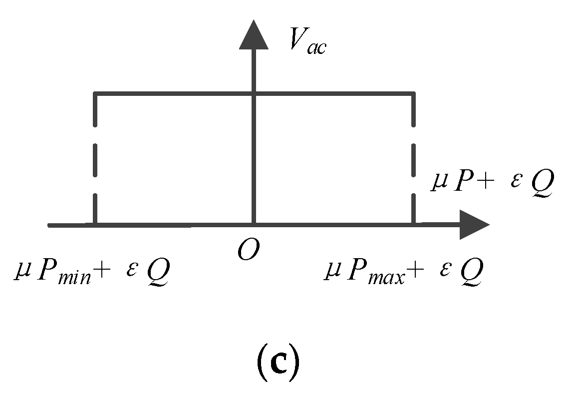
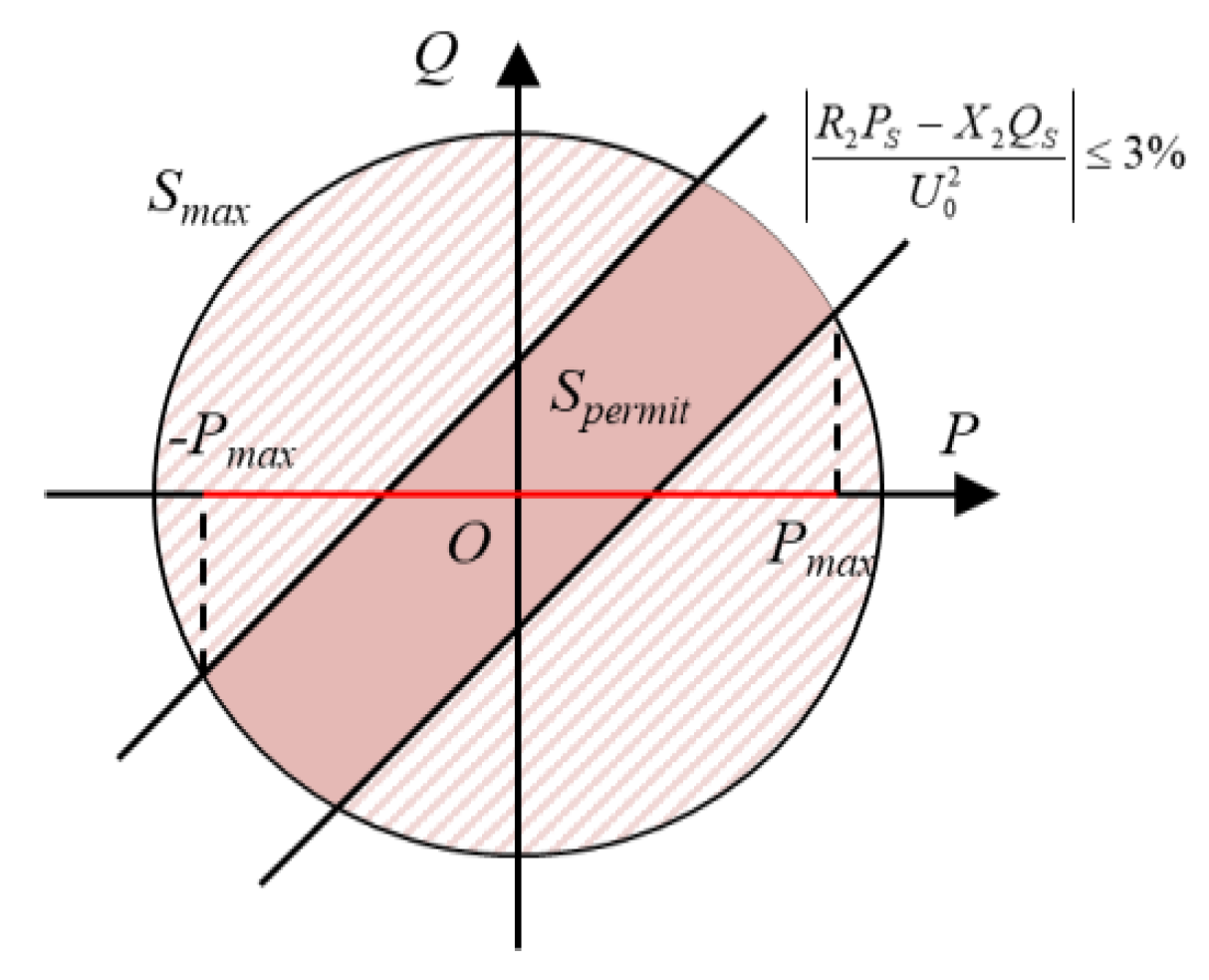
Taking both the active and reactive power of SOP into consideration to regulate the voltage of feeder nodes based on the line impedance, which can fully utilize the apparent power of SOP.
(2)
Achieving the goal of saving the computation and communication costs, and the local control proposed can respond rapidly to voltage fluctuation compared with the traditional global optimization control.
The remainder of this paper is organized as follows. Section 2 establishes the SOP math model, and analyzes the principle of power regulation. Section 3 simplifies the model of the low-voltage distribution network by using the impedance characteristics of a low-voltage distribution network to establish a fast local non-communication control strategy, which aims to reduce the impact of new energy access on the voltage of the feeder nodes. Section 4 carries out the simulation analysis to verify the control effect.

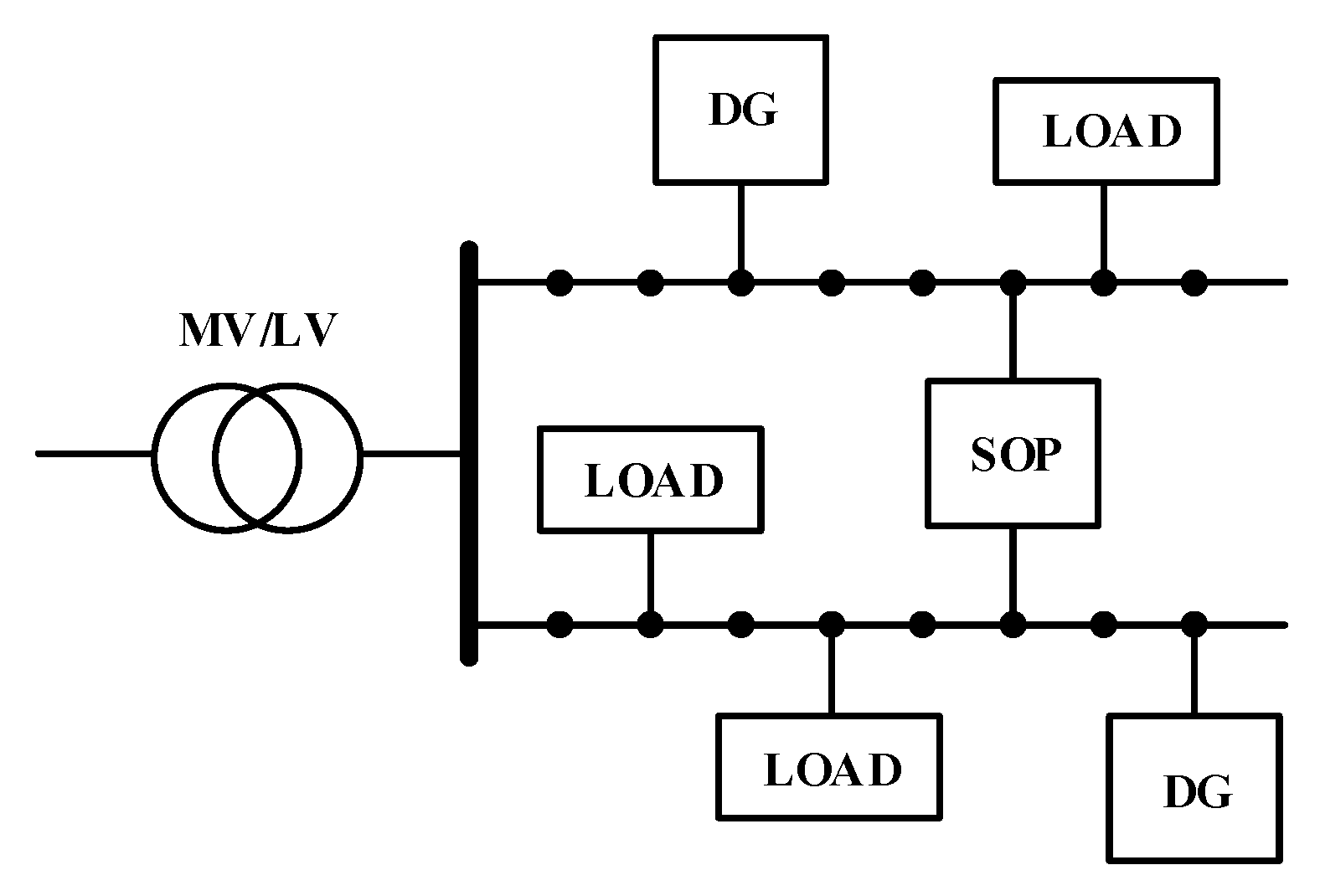
2. System Modeling and Analysis

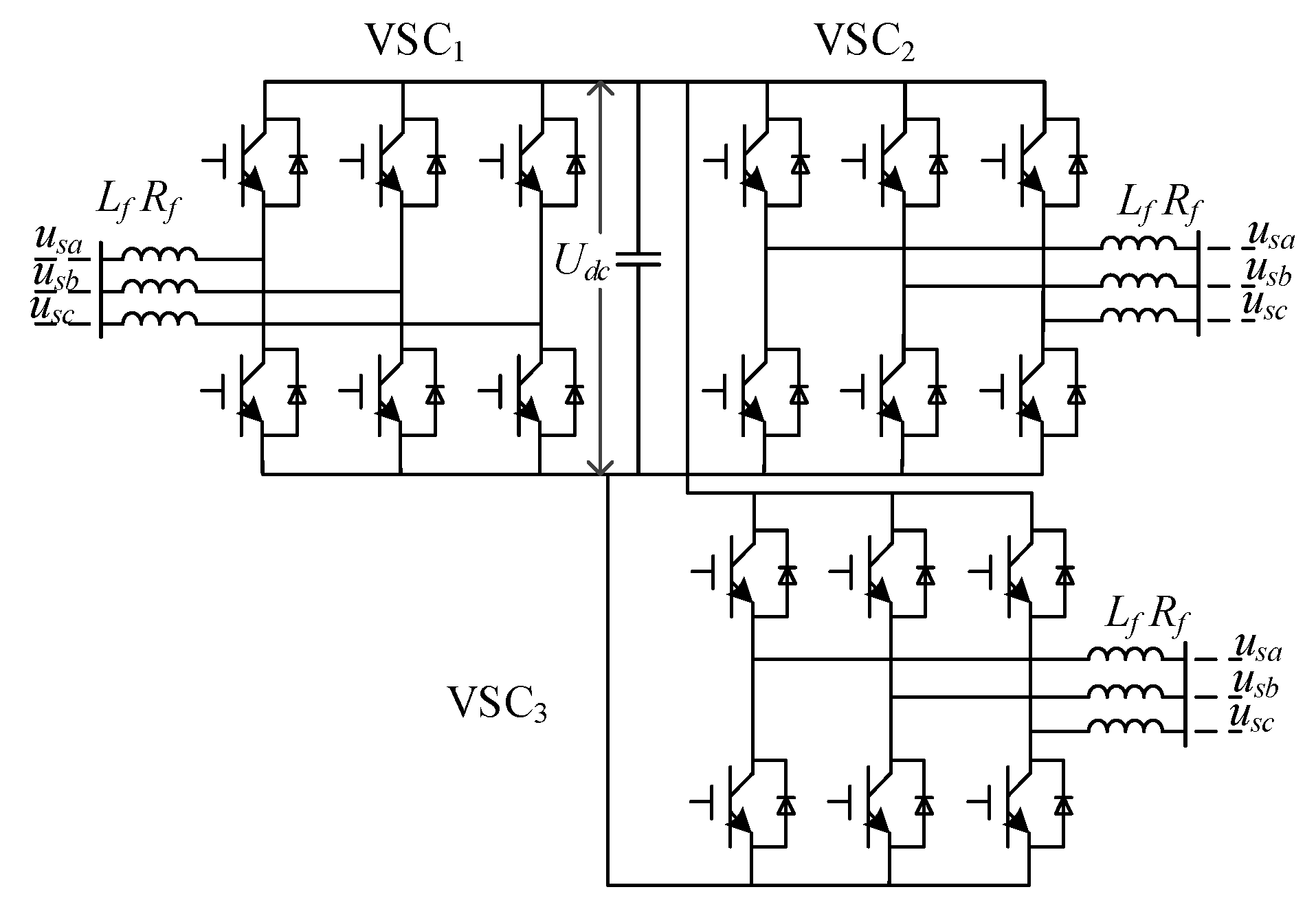
2.1. Modeling of Soft Open Points

The typical application of SOP is shown in Figure 1. The SOP monitors the voltage between the terminal of itself. If the voltage exceeds the reference, it will change the flow direction of the active power to balance the feeders. The SOP topology is shown in Figure 2. u s j is the phase voltage at the point of common coupling in the grids (PCC), U d c is the SOP bus voltage, and L f and R f are the converter inductance and equivalent resistance. The loop voltage equation at one terminal of SOP can be established by the Kirchhoff voltage law:
u s j + L f d i j d t + R f i j = m j U d c j = a , b , c u s j + L f d i j d t + R f i j = m j U d c j = a , b , c .
As the three converters have the same parameters, one phase can be used to represent the other two converters. Equation (1) is a soft open pointing differential equation in steady state, and in the equation, m j is the modulation ratio of the converter.
In the state of three-phase equilibrium, the equation of the three-phase signal can be converted to a two-phase rotating coordinate system, using the Park’s transformation. As a result, the matrix expression in the DQ coordinate system can be obtained:
[ u s d u s q ] + L f d d t [ i d i q ] + R f [ i d i q ] + L f [ 0 ω ω 0 ] [ i d i q ] = U d c [ m d m q ] .
According to the instantaneous reactive power theory, the instantaneous active power and reactive power injected into the AC system can be expressed as:
[ p s q s ] = 3 2 [ u s d u s q u s q u s d ] [ i d i q ] [ p s q s ] = 3 2 [ u s d u s q u s q u s d ] [ i d i q ] .
In a steady state, the q-axis component of the network voltage measurement is zero, so Equation (3) can be simplified to:
{ p s = 3 2 u s d i d q s = 3 2 u s d i q .
From Equation (4), it can be concluded that the active and reactive power of the converter can be controlled by decoupling the current in the DQ axis, which lays the foundation for subsequent hybrid power compensation.
Assuming that the DC bus voltage is stable, the active power of the three terminals should be balanced, which can be expressed as:
P S 1 + P S 2 + P S 3 = 0 .
From Equation (5), it can be concluded that the SOP itself cannot generate active power. Once the electronic convert of SOP at a feeder regulates the terminal active power, other cooperation is needed. Therefore, it is necessary to establish the external characteristic model of the soft open point access network strategy and further study the active power distribution.

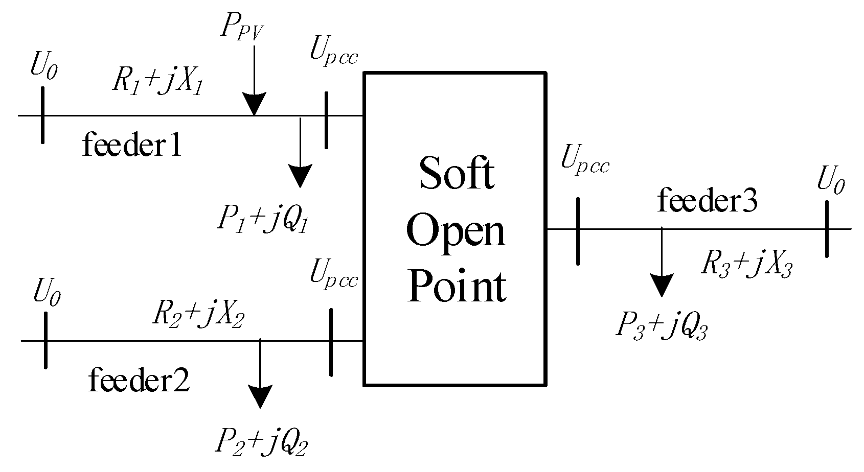
2.2. Local Network Modeling

Taking the photovoltaic power generation system as an example, there are three low-voltage distribution feeders that derive from different distributed networks. Two of them are connected to the photovoltaic distributed generations. If the active power emitted by the photovoltaic is higher than that required by the load, the power flow of the distribution network will turn back to the distributed networks, resulting in unnecessary line loss. In order to suppress the active power fluctuation, the feeders with photovoltaic generation and supportive feeders are connected to the SOP. The excess active power can be transferred to the supportive feeder through SOP to achieve the absorption of renewable energy sources.
The feeder model mentioned above is simplified as shown in Figure 3. All the loads after the photovoltaic access point of feeder 1 are equivalent to P 1 + j Q 1 , and the equivalent feeder line impedance is R 1 + j X 1 . In this paper, we consider the worst situation for renewable generation. The reactive power output of the inverter is neglected, and the active power is the dominant output. The photovoltaic access power is equivalent to PPV. The line impedance of feeder 2 is R2+jX2, and the load equivalent is P 2 + j Q 2 . The line impedance of feeder 3 is R 3 + j X 3 , and the load equivalent is P 3 + j Q 3 .
Before the soft open point is connected, according to the line impedance and the distribution of load in Figure 3, the voltage at the PCC of the line is as follows:
U P C C = U 0 R 1 ( P 1 P P V ) + X 1 Q 1 U 0 .
According to [11], a low-voltage distribution network has two distinct characteristics: (1) Higher r/x of line, and (2) radial topology. Because of the high r/x of low-voltage lines, the decoupling relationship in the active power to thee phase angle and reactive power to voltage no longer exists. As a result, both active and reactive energy have a significant impact on the voltage. For the lines with r>x, the sensitivity of the active power to the voltage is greater than that of the reactive power to the voltage; that is, the effect of active power on voltage is more significant. Therefore, when the active power of the photovoltaic output fluctuates rapidly, the voltage at PCC fluctuates accordingly.
At present, the SOPs used at the end of the feeder are mostly multi-terminal, with which active power is coupled. However, the terminal voltage is only affected by the terminal power. If the power transferred by the soft open point connected to feeder 1 is P S and the reactive power generated independently is Q S , the voltage at PCC of the feeder can be obtained as follows:
U P C C = U 0 R 1 ( P 1 P P V P S 1 ) + X 1 ( Q 1 Q S 1 ) U 0 .
In theory, as long as the numerator R 1 ( P 1 P p v P s 1 ) + X 1 ( Q 1 Q S 1 ) in Equation (7) is kept at zero, the compensation demand can be met.
The influence of the active power on the voltage of feeder 2 and 3 can be expressed as follows:
U P C C = U 0 R 2 , 3 ( P 2 , 3 + P S 2 , S 3 ) + X 2 , 3 ( Q 2 , 3 Q S 2 , S 3 ) U 0 .
Equation (8) shows that the voltage fluctuation of feeder 2 and 3 will be increased by compensating feeder 1. Therefore, to maintain the voltage balance of feeder 2 and 3, on the one hand, the maximum active power transmission should be limited; on the other hand, the reactive power should be compensated to a certain extent.
From the above two equations, it can be seen that the voltage of the feeder node is affected by the active power and reactive power of the load, power supply, and soft open point. So, adjusting the active and reactive power output of the soft open point can weaken the influence of the distributed energy and load on the voltage of the feeder.

3. Distributed Energy Fluctuation Suppression Strategy

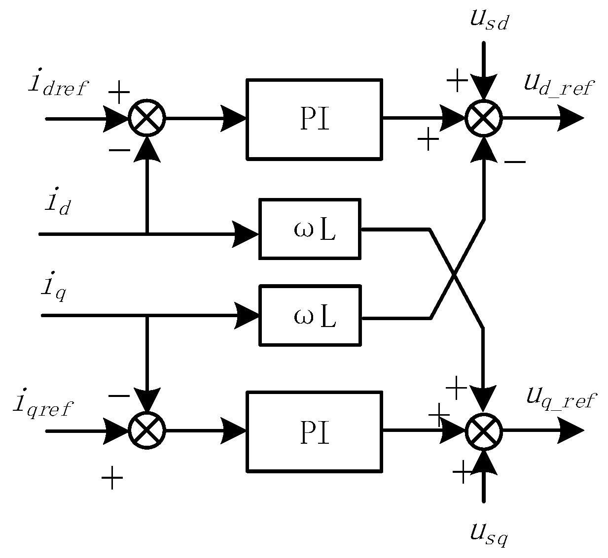
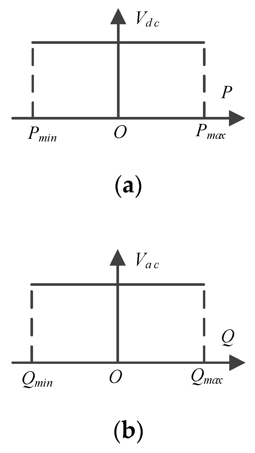
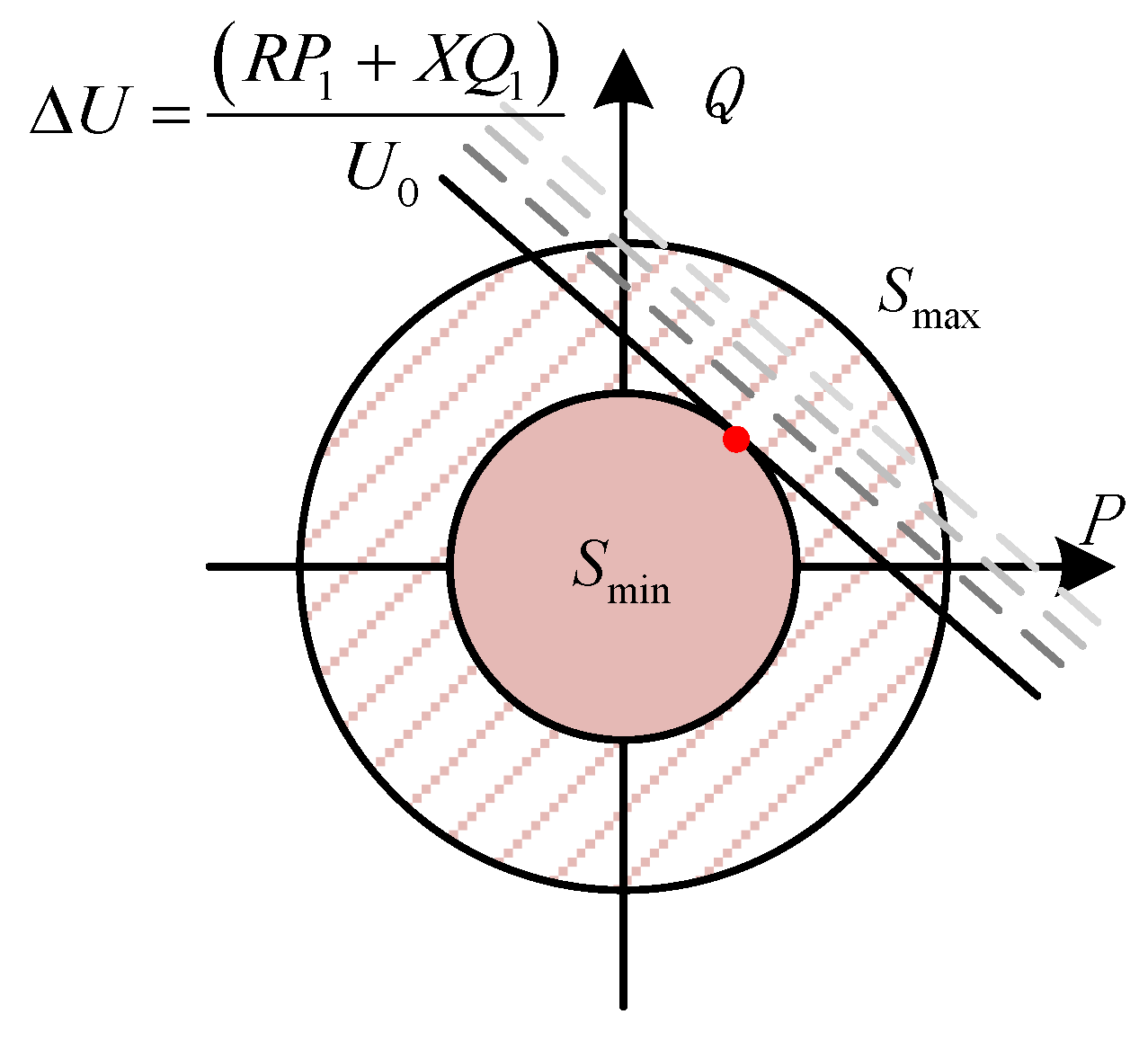
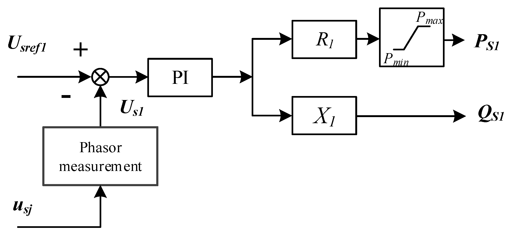
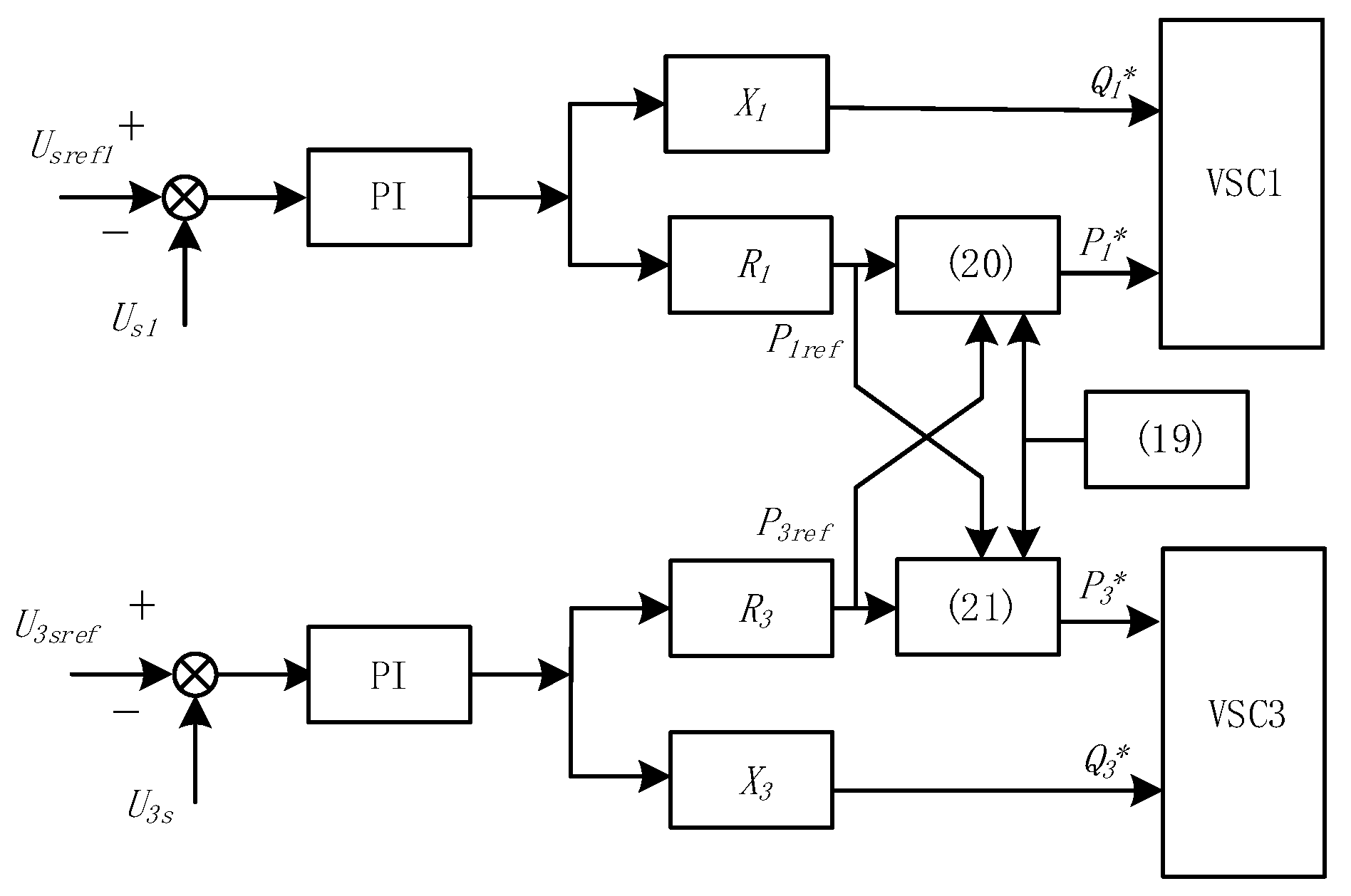
3.1. Converter Control Strategy

In this section, the inner control strategy of SOP is established. It can be seen from Equation (2) that the current of the convert is coupled in the equation after Park’s transformation, so decoupling control should be considered in the design of the current loop, as shown in Figure 4. The D-axis and Q-axis currents given by the outer loop subtract the grid-side currents, and are then fed to the PI regulator. The compensative signal of the DQ axis current multiplied by the impedance ( L f i d q ) is added to the output of the current loop to eliminate the coupling caused by the Park’s transformation. In addition, the feeder PCC voltage signal ( u s d q ) is added to eliminate the influence of the grid voltage. The output DQ axis reference voltage signal ( u s d q _ r e f ) is converted by inverse Park’s transformation to output the controllable AC modulation signal. With the access of the distributed energy, SOP needs to monitor the voltage changes of the power grid in real time, and the current should be compensated without delay. Therefore, the bandwidth of the current loop needs to be broad, which can provide high feedback gain for large-scale signals.
For the outer loop control strategy, the diversity of control objectives should be considered. As the Park’s transformation can decouple active and reactive currents, the controller is often divided into active power and reactive power regulation in the design of the outer loop.
Figure 5a is classified as the active power regulation curve, adjusting the d-axis current ( i d _ r e f ) in Figure 4. It mainly ensures the internal DC voltage of SOP is stable. Figure 5b is the active power regulation curve, adjusting the q-axis current ( i q _ r e f ) in Figure 4. It mainly ensures the external AC voltage of SOP is stable. It can be inferred that the reactive power should mainly suppress the voltage at PCC of the feeder. However, this control method only make sense in a low r/x distributed network. In the high r/x distributed network, the fluctuation of active power will cause more voltage to be unstable. Therefore, a hypothesis is formulated that a mixed control strategy would perform better, as shown in Figure 5c. There are two undetermined coefficients μ and ε , which will be calculated in the next section.

3.2. Feeder Voltage Control Strategy

A previous study [12] lists the optimization equation of SOP. It uses a genetic algorithm to calculate power regulation. However, in a low-voltage distribution network, the communication network is unsatisfactory and the reliability is low [13]. It does not have the condition of collecting all nodes’ information like that in a medium-voltage distribution network for global optimization.
Because of the high line impedance, optimization and compensation are not suitable for remote implementation, so a local compensation control strategy is needed to adjust the operation mode of the multi-terminal soft open point based on different requirements.
(1) Minimum apparent power control
The impedance ratio r/x of the terminal line of a low voltage distribution network is high. The active and reactive power of the load or distributed energy can affect the voltage of the common connection point (PCC) at the same time. How to optimize the power output of SOP is a problem to be solved in the local control strategy. In order to quantify the effect of these variables on the common connection points, the PCC voltage in Equation (6) is taken as partial derivatives by the active and reactive power, respectively:
U P C C P = R 1 U 0 ,
U P C C Q = X 1 U 0 .
Equations (9) and (10) show that the resistance value of the feeder determines the effect of the active power on the line voltage, and the reactance value of the feeder determines the effect of the reactive power on the line voltage. Therefore, an optimal problem arises. This paper proposes a control strategy to distribute the converter power reasonably by using the actual line impedance value to achieve the maximum utilization ratio of the converter capacity. The detailed analysis is as follows:
m i n S = P S 1 2 + Q S 1 2 subject   to Δ U = ( R 1 P S 1 + X 1 Q S 1 ) U 0 P S 1 2 + Q S 1 2 S m a x 2 P S 1 P S 2 m a x P S 3 m a x .
Equation (11) shows that in the case of photovoltaic power fluctuation at one end, power support is provided by the other two ends, and there is a minimum apparent power condition for one end converter:
m i n S 1 = P S 1 2 + Q S 1 2 S 3 = P S 3 2 + Q S 3 2 subject   to Δ U 1 = ( R 1 P S 1 + X 1 Q S 1 ) U 0 Δ U 3 = ( R 3 P S 3 + X 3 Q S 3 ) U 0 P S 1 2 + Q S 1 2 S m a x 2 P S 3 2 + Q S 3 2 S m a x 2 P S 1 + P S 3 P S 2 m a x .
Equation (12) indicates that in the case of fluctuation of the photovoltaic power at both ends, the third end supports all the active power. A minimum apparent power of the two-end converter exists on the premise of satisfying the active power constraints.
The power circle is an effective method for analyzing the SOP. As shown in Figure 6, the outer circle enclosure area is the maximum apparent power of the converter, and the family of functions in the diagram is the corresponding compensation function under different voltage drops Δ U . Under the limitation of the maximum apparent power and compensation curve, the minimum apparent power utilization of the converter is the red point, where the apparent power circle is tangent to the compensation function. In other words, when the static working point satisfies Equation (13), the converter achieves the minimum apparent power condition:
Q S = X 1 R 1 P S .
Therefore, in the design of a local control strategy, active and reactive power regulations share a voltage loop. As shown in Figure 7, the phasor measurement takes the time-domain voltage u s j into the aptitudes of it. Though the PI controller, the outputs are respectively multiplied by the coefficient of Equation (13) to synchronously regulate the voltage.
(2) Mode switching strategy
The local control of SOP requires not only the minimum apparent power control of the converter but also the suitable switching strategy of the converter under different conditions.
Equation (5) shows that the SOP can compensate for the power fluctuation at one end or both ends. However, it does not have an energy storage structure. The power control has only two degrees of freedom. As a result, it can suppress the photovoltaic fluctuation on, at most, two feeders. Two effective modes are discussed in the next paragraph.
Mode 1: A feeder has photovoltaic power generation. Assuming that the feeder connected to the photovoltaic power generation has adopted minimum apparent power compensation, the active power transferred is P 1 , the supportive active power of feeder 2 is P 2 , and the supporting active power of feeder 3 is P 3 . The voltage fluctuation of the support feeder can be expressed as a standard deviation:
m i n σ 2 ( Δ U 2 ) + σ 3 ( Δ U 3 ) s u b j e c t   t o P S 1 = P S 2 + P S 3 Δ U 2 = R 2 P S 2 U 0 Δ U 3 = R 3 P S 3 U 0
Equation (14) pays attention to the effect of the active power on the voltage of the supporting feeder. It shows that different line resistors have different voltage variation rates, which means that smaller feeder resistances can support more active power in the same range of voltage fluctuation. Therefore, the sum of standard deviations of voltage fluctuations for feeder 2,3 is the smallest when Equation (15) is satisfied for the feeder support:
R 2 P 2 = R 3 P 3 .
It can be seen from Equation (15) that if the voltage fluctuations of the two supporting feeders are consistent, the power distribution should be carried out according to the line impedance. The active power support reference values of feeder 2 and feeder 3 can be obtained from the simultaneous Equations (5) and (15):
P 2 = P 1 R 3 R 2 + R 3 ,
P 3 = P 1 R 2 R 2 + R 3 .
Mode 2: Photovoltaic power generation exists in the two feeders, such as feeder 1 and 3. In this mode, the power demand of feeder 1 and 3 is determined by the minimum apparent power control loop, and the supportive power of feeder 2 is determined due to the power balance. It can be controlled by the V d c Q control strategy. However, there is a problem in this mode; that is, the supportive feeder may risk overvoltage due to the overactive power support. Therefore, it is necessary to add active power saturation in the control loop of the supportive converter. First, it is necessary to calculate the influence of the active power transferred by SOP on the voltage of feeder 2:
Δ U P C C = | R 2 P S X 2 Q S U 0 2 | .
Equation (18) is the fluctuation voltage generated by SOP on feeder 2. For the random and irregular voltage fluctuation, the limit value of the low-voltage distribution network is 3%. Therefore, it is necessary to limit the active power derived from feeder 2. That is, Equation (18) is less than 3%.
Limited by the fluctuating voltage of feeder 2, the active power transmitted by SOP is bounded. As shown in Figure 8, the overlapping part between the equation of the fluctuation voltage limitation and the maximum apparent power is the transmission power feasible region, and the junction point is the transmission active power boundary: P m a x and P m a x .
The active power at the boundary of Equation (11) is calculated by solving the algebraic equation:
P m a x = S s i n ( 2 a r c t a n ( R 2 S R 2 2 S 2 + X 2 2 S ( 0.03 U 0 2 + X 2 S ) 0.03 U 0 2 X 2 S ) ) .
In mode 2, the transmission boundary of the active power support from feeder 2 under the premise of reactive power compensation is Equation (19), and the corresponding reactive power value can be calculated by Equation (12). Therefore, when the sum of active power required by feeder 1 and feeder 3 exceeds the maximum active power provided by feeder 2, the voltage fluctuation rate can be sacrificed appropriately to limit the transfer power so as to stabilize the node voltage of the DC bus and feeder 2:
P 1 * = { P 1 r e f | P 1 r e f + P 3 r e f | < P 2 m a x P 2 m a x P 1 r e f + P 3 r e f P 1 r e f | P 1 r e f + P 3 r e f | P 2 m a x ,
P 3 * = { P 3 r e f | P 1 r e f + P 3 r e f | < P 2 m a x P 2 m a x P 1 r e f + P 3 r e f P 3 r e f | P 1 r e f + P 3 r e f | P 2 m a x .
In Equations (20) and (21), P1ref and P3ref are the active power reference values of the voltage control output while P 1 * and P 3 * are the reference values of the actual output to the power loop after limitation. Feeder 2 adopts constant DC voltage control, so its active reference values P 2 * are determined by the demand of VSC1 and VSC3. The complete outer loop control loop is shown in Figure 9. Under this condition, the sum of the transformation active power of the two feeders will not exceed the supportive power limit of feeder 3.

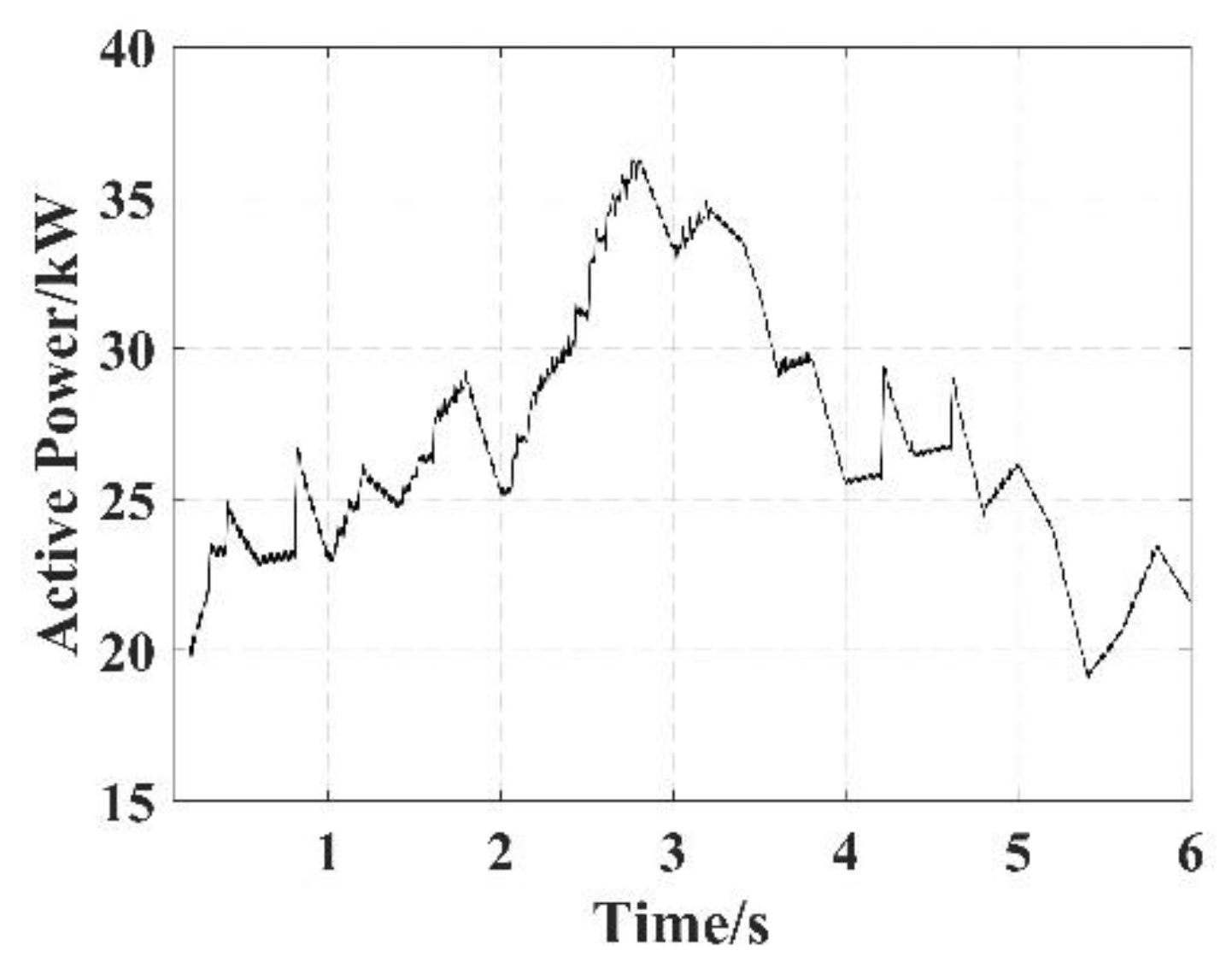
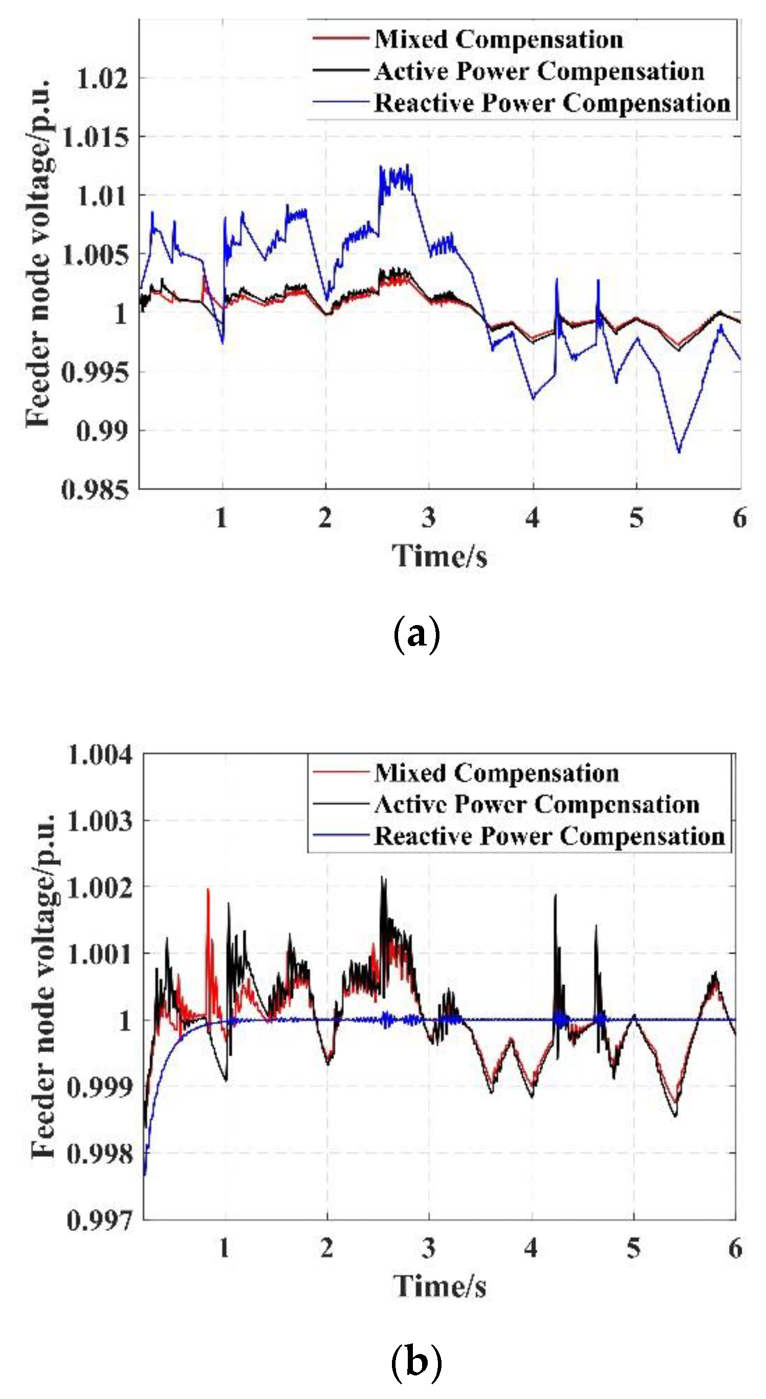
4. Simulation Analysis

Using MATLAB/Simulink simulation software, the model of SOP connecting to a low-voltage distribution network was established. The line adopted a LGJ-35 steel-cored aluminum strand with a resistance of 0.85 /km, reactance of 0.366 /km, line impedance ratio of r/x of 2.322, and line length of 1 km. The feeder 1 load was 20 kW rated active power and 1 kvar rated reactive power. Feeder 2 load was 15 kW rated active power, 1 kvar rated reactive power. Feeder 3 load was 10 kW rated active power, 1 kvar rated reactive power. The main parameters of the converter are: AC filter inductance L f = 250 μH, inductance equivalent resistance Rf = 2mΩ, DC capacitor 6mF, three-phase AC line voltage effective value 380V, DC voltage 400V.
Taking the city office building with photovoltaic self-generating as an example, the characteristic is that the load and photovoltaic power were concentrated. In total, 125 photovoltaic blocks were connected in series and parallel. The maximum output power was 38 kW. Under the condition of random fluctuation of light and temperature, the maximum power tracking algorithm was adopted. The active power output of photovoltaic inverters was obtained by simulation as shown in Figure 10.
It can be seen that the active power output of the photovoltaic inverters fluctuates rapidly in 6 s, reaching a maximum of 32 kW and a minimum of 15 kW. The frequency of photovoltaic output fluctuation is mainly distributed in 0.1 to 1Hz, which accounts for 92.1% in the system. This means the SOP has enough time to compensate the feeder voltage.

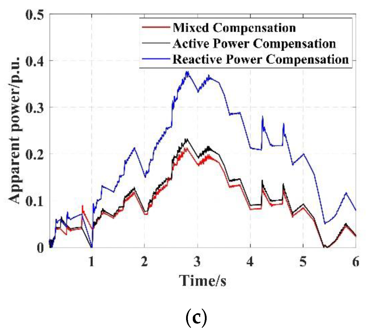
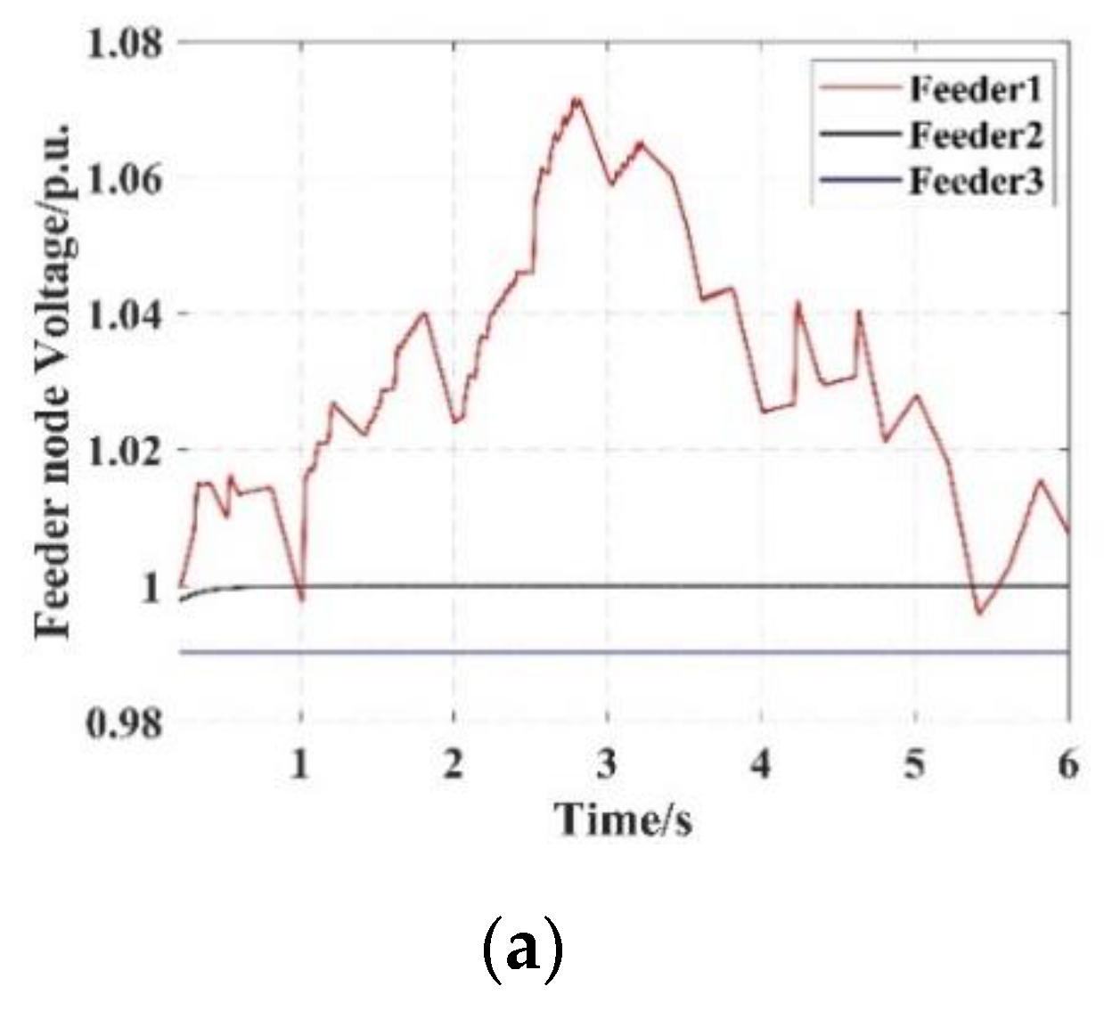
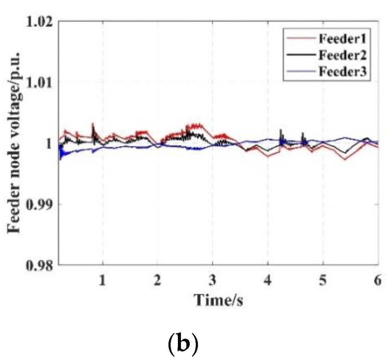
4.1. Verification of Minimum Apparent Power Compensation for Soft Open Point

SOP is composed of bidirectional converters, which can transfer active power bidirectionally and actively generate reactive power. This simulation aimed to verify that the mixed compensation has a better performance than the sole compensation in a low voltage feeder with a high impedance ratio r/x.
In this simulation example, feeder 1 was connected to a photovoltaic power generation. The effects of three voltage compensation methods, reactive power compensation, active power compensation, and minimum apparent power compensation (mixed compensation), were compared. Figure 11a shows that the maximum PCC voltage deviation under reactive power compensation is 2.8%, the maximum PCC voltage deviation under active power compensation is 0.8%, and that under the mixed compensation is 0.8%. In Figure 11c, the maximum apparent power consumption under reactive power compensation is 0.278 p.u., the maximum apparent power consumption under active power compensation is 0.199 p.u., and that under the mixed compensation consumption is 0.184 p.u.
It can be analyzed as follows:
(1) In a low voltage distribution network with the line resistance greater than the inductance, the compensation effect of the active power on the line voltage is better than that of the reactive power. However, if active power compensation is used solely, it will lead to larger pressure on other feeders that derive active power. In Figure 11b, feeder 2 provides active support to feeder 1, and the voltage fluctuation of feeder 2 is 0.7%, the same as that of feeder 2. The voltage fluctuation caused by hybrid compensation is 0.5%. It can be seen that the voltage fluctuation of feeder 1 and 2 is well balanced by mixed compensation.
(2) Active power compensation and mixed compensation consume lower apparent power on the premise of having the same voltage compensation effect, which can reduce the cost of equipment to a certain extent.

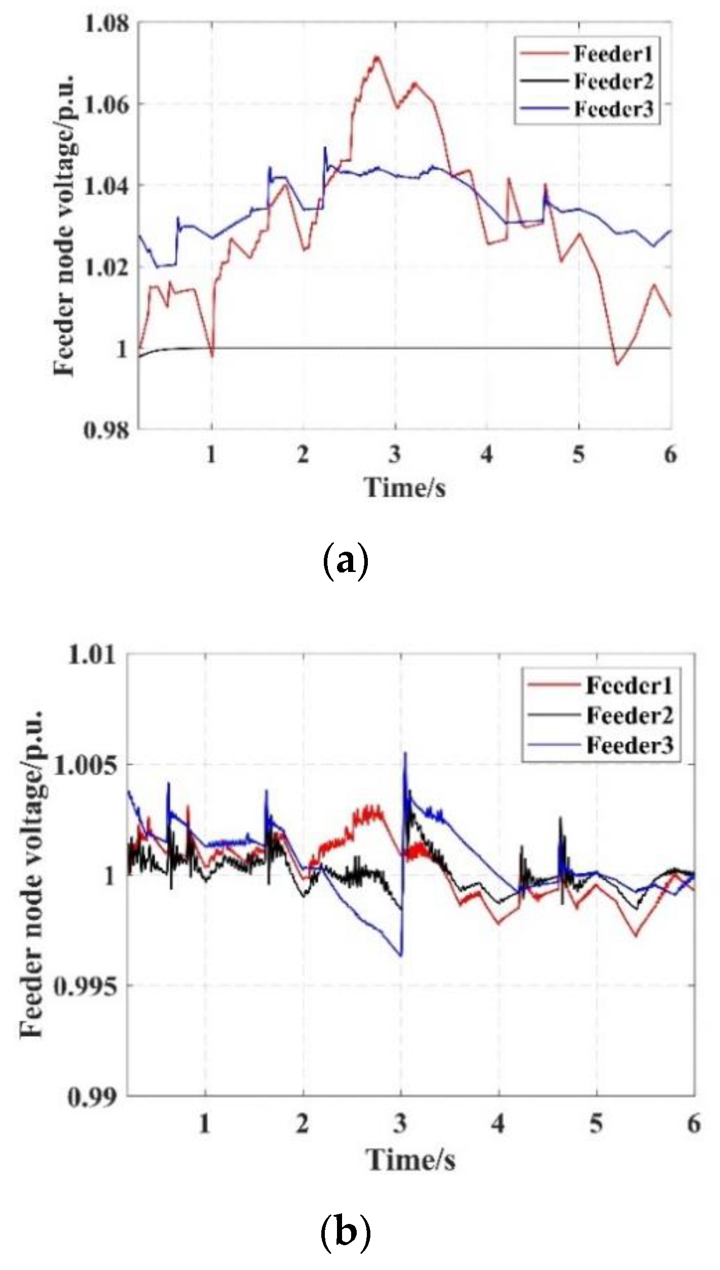
4.2. Verification of Mode Switching for SOP

(1) Photovoltaic access to one node
In this simulation example, the feeder 1 was connected to a photovoltaic power generation and feeder 2 and 3 are supportive feeders. As shown in Figure 12a, without soft open point, the voltage fluctuation of feeder 1 exceeded 7%, which risks the voltage exceeding the limit. When the SOP is committed, as shown in Figure 12b, the voltage fluctuation is divided equally into the remaining feeders. As can be seen from Table 1, the standard deviation of feeder 1 was reduced by 92.6%. The active power fluctuation caused by photovoltaic is suppressed.
Before the soft open point is connected, according to the line impedance and the distribution of load in Figure 3, the voltage at the PCC of the line is as follows.
(2) Photovoltaic access to both nodes
In this simulation example, the feeders 1 and 3 were connected to photovoltaic power generations and the feeder 2 and 3 were supportive feeders. As shown in Figure 13a and Table 2, on the condition that both feeder 1 and feeder 3 were connected to the photovoltaic, feeder 1 has a risk of overvoltage and feeder 3 is close to the edge of overvoltage. When SOP is committed, as shown in Figure 13b and Table 2, the standard deviation of feeder 1 decreases by 93%, and that of feeder 3 decreases by 86%. The random voltage fluctuation is less than 1%. This means that the distributed energy is greatly suppressed, which meets the requirements of the power grid.

5. Conclusions

In this paper, a local control strategy applied to the multi-terminal SOP was proposed to suppress renewable energy generation fluctuation. Based on the characteristic of line resistance and inductance, the active and reactive power can be regulated at the same time, as the former mainly balances the two terminal voltages whereas the latter keeps the voltage close to rated. Compared with the existing single reactive power compensation strategy based on a photovoltaic converter, the result showed that mixed compensation based on SOP performs better in voltage suppression and consumes less apparent power in a low-voltage distributed grid. In addition, the proposed local control strategy can respond rapidly to address the uncertainties of DG outputs compared to the traditional strategy. In general, the SOP intervention provides more power output space for renewable energy generation, which boosts the adoption of it.
The limitation of the study is that the model of the distributed network is bounded, and the number of SOP is finite, which means once the distributed network becomes larger and more complex, this method may not achieve the optimal result. Therefore, broadening of the simulated network and the application of more SOPs will be the next direction of this research.

Author Contributions

G.X. conceived and designed the study; Y.J., W.T. and H.Q. have given suggestions and revised the manuscript. All authors have read and agreed to the published version of the manuscript.

Funding

Project supported by National Natural Science Foundation of China (51607171), Chinese Academy of Sciences Youth Innovation Association (2017180), Research on the coordinated control technology of PET and FCL in AC / DC system(j2019131), China Postdoctoral Science Foundation (2019M652028).

Conflicts of Interest

The authors declare no conflict of interest.

Nomenclature

mjModulation ratio of the SOP
indices usd, usq(usdq)Voltage source of PCC in DQ form
jPhase a, b and cid, iqOutput current of converter in DQ form
iIndices of nodes, from 1 to 3ps, qsActive and reactive power of the SOP
Variables usdq_refReference voltage of PCC in DQ form
Pi, QiActive and reactive power of load in feeder iParameters
PPVActive power of photovoltaic generationμ, εundetermined coefficient of control
PSi, QSiActive and reactive power of SOP in feeder iUsrefReference voltage of PCC
UPCCVoltage at the point of common couplingRf, LfResistance and Inductance of SOP
SmaxThe maximum apparent power of SOPUdcSOP bus voltage
PSimaxThe maximum active power of SOPRi, XiEquivalent line resistance and inductance
usjVoltage source of PCCU0Voltage at the secondary side of the transformer
ijOutput current of SOP

References

  1. Narayan, S.; Doytch, N. An investigation of renewable and non-renewable energy consumption and economic growth nexus using industrial and residential energy consumption. Energy Econ. 2017, 68, 160–176. [Google Scholar] [CrossRef]
  2. Bloemink, J.M. Increasing distributed generation penetration using soft normally-open points. In Proceedings of the Power & Energy Society General Meeting, Providence, RI, USA, 25–29 July 2010; pp. 1–8. [Google Scholar]
  3. Huo, Q.; Su, M.; Wu, L.; Wei, T.; Wang, P. Compound Control Strategy for Soft open point. Autom. Electr. Power Syst. 2018, 42, 166–170. [Google Scholar]
  4. Ji, H.; Wang, C.; Li, P.; Zhao, J.; Song, G.; Wu, J. Quantified Flexibility Evaluation of Soft Open Points to Improve Distributed Generator Penetration in Active Distribution Networks Based on Difference-of-Convex Programming. Appl. Energy 2018, 218, 338–348. [Google Scholar] [CrossRef]
  5. Qi, Q.; Wu, J.; Long, C. Multi-Objective Operation Optimization of an Electrical Distribution Network with Soft Open Point. Appl. Energy 2017, 208, 734–744. [Google Scholar] [CrossRef]
  6. Yao, C.; Zhou, C.; Yu, J.; Xu, K.; Li, P.; Song, G. A Sequential Optimization Method for Soft Open Point Integrated with Energy Storage in Active Distribution Network. Energy Procedia 2018, 145, 528–533. [Google Scholar] [CrossRef]
  7. Ji, H.; Yu, H.; Song, G.; Li, P.; Wang, C.; Wu, J. A decentralized voltage control strategy of soft open points in active distribution networks. Energy Procedia 2019, 159, 412–417. [Google Scholar] [CrossRef]
  8. Li, P.; Ji, H.; Song, G.; Yao, M.; Wang, C.; Wu, J. A Combined Central and Local Voltage Control Strategy of Soft Open Points in Active Distribution Networks. Energy Procedia 2019, 158, 2524–2529. [Google Scholar] [CrossRef]
  9. Li, P.; Ji, H.; Yu, H.; Zhao, J.; Wang, C.; Song, G.; Wu, J. Combined decentralized and local voltage control strategy of soft open points in active distribution networks. Appl. Energy 2019, 241, 613–624. [Google Scholar] [CrossRef]
  10. Zheng, Y.; Song, Y.; Hill, D.J. A general coordinated voltage regulation method in distribution networks with soft open points. Int. J. Electr. Power Energy Syst. 2020, 116, 105571. [Google Scholar] [CrossRef]
  11. Cai, Y.; Tang, W.; Xu, O.; Zhang, L. Review of Voltage Control Research in LV Distribution Network With High Proportion of Residential PVs. Power Syst. Technol. 2018, 42, 220–229. [Google Scholar]
  12. Cao, W.; Wu, J.; Jenkins, N.; Wang, C.; Green, T. Operating principle of Soft Open Points for electrical distribution network operation. Appl. Energy 2016, 164, 245–257. [Google Scholar] [CrossRef] [Green Version]
  13. Long, C.; Wu, J.; Thomas, L.; Jenkins, N. Optimal operation of soft open points in medium voltage electrical distribution networks with distributed generation. Appl. Energy 2016, 184, 427–437. [Google Scholar] [CrossRef] [Green Version]
Figure 1. A typical application of soft open point.
Energies 13 01520 g001
Figure 2. Three-terminal soft open point.
Energies 13 01520 g002
Figure 3. Soft open point access network.
Energies 13 01520 g003
Figure 4. Inner loop control strategy of soft open point.
Energies 13 01520 g004
Figure 5. Outer-loop control strategy of SOP: (a) Active power regulation to DC voltage; (b) Reactive power regulation to AC voltage; (c) mixed regulation to AC voltage.
Energies 13 01520 g005aEnergies 13 01520 g005b
Figure 6. Principle of minimum apparent power.
Energies 13 01520 g006
Figure 7. Power delivery based on minimum apparent power control.
Energies 13 01520 g007
Figure 8. Transmission power boundary of SOP.
Energies 13 01520 g008
Figure 9. Local control strategy of SOP.
Energies 13 01520 g009
Figure 10. Photovoltaic active power fluctuation.
Energies 13 01520 g010
Figure 11. Effect of different compensation modes for SOP: (a) Voltage at the end of feeder 1; (b) Voltage at the end of feeder 2; (c) Apparent power consumption.
Energies 13 01520 g011aEnergies 13 01520 g011b
Figure 12. Feeder node voltage in mode 1: (a) SOP is uncommitted into operation; (b) Soft open point is committed into operation.
Energies 13 01520 g012aEnergies 13 01520 g012b
Figure 13. Feeder node voltage in mode 2: (a) SOP is uncommitted to operation; (b) Soft open point is committed to operation.
Energies 13 01520 g013
Table 1. Standard deviation of feeder node voltage.
Switching StateFeed 1Feed 2Feed 3
uncommitted0.01891e-63.3e-7
committed0.00140.00210.0021
Table 2. Standard deviation of the feeder node voltage.
Switching StateFeed 1Feed 2Feed 3
uncommitted0.01841.5e-70.0059
committed0.00130.00150.0008

