Performance Evaluation of Wire Cloth Micro Heat Exchangers

 ,
,
Abstract
:
1. Introduction
2. Methods
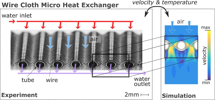
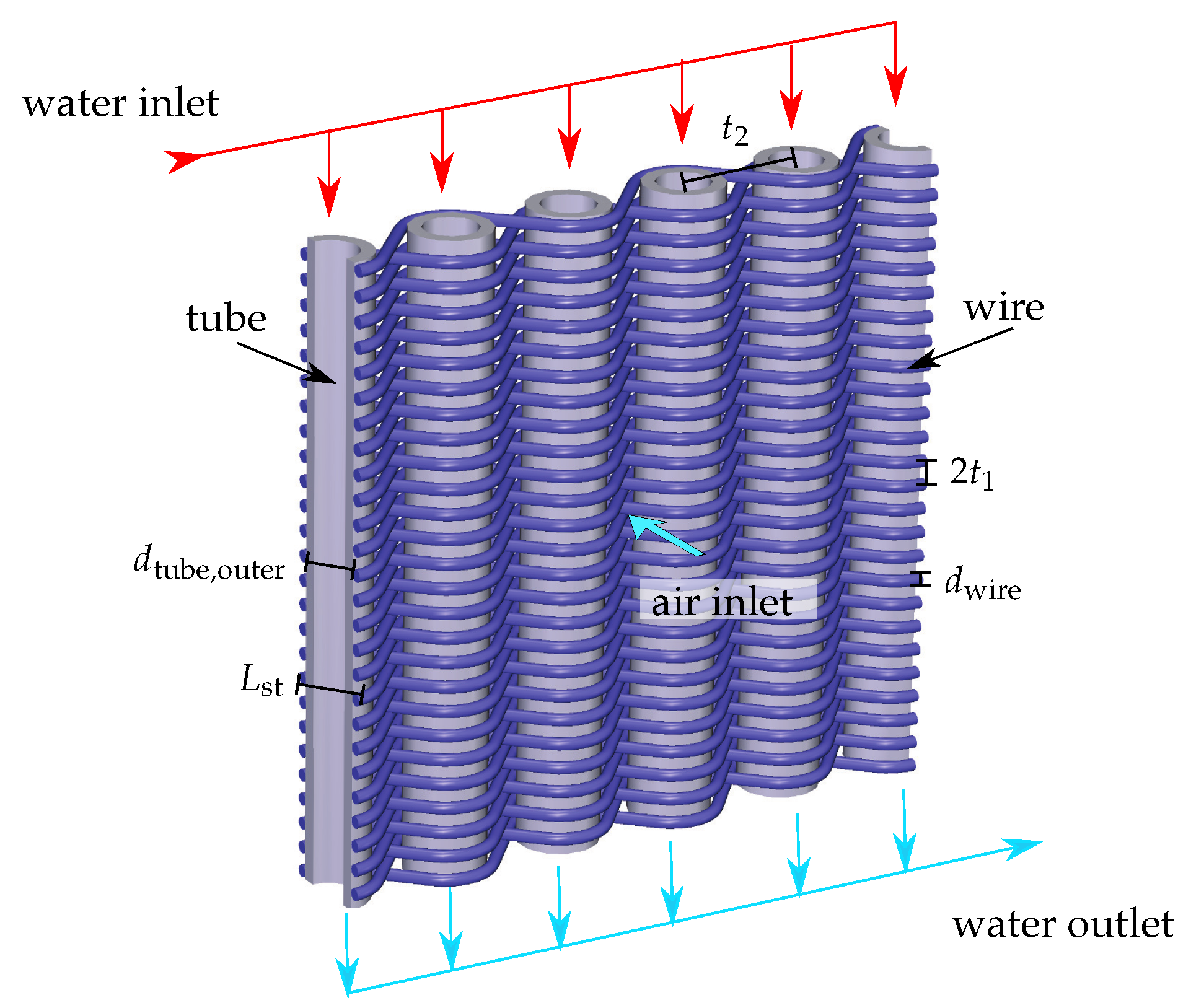
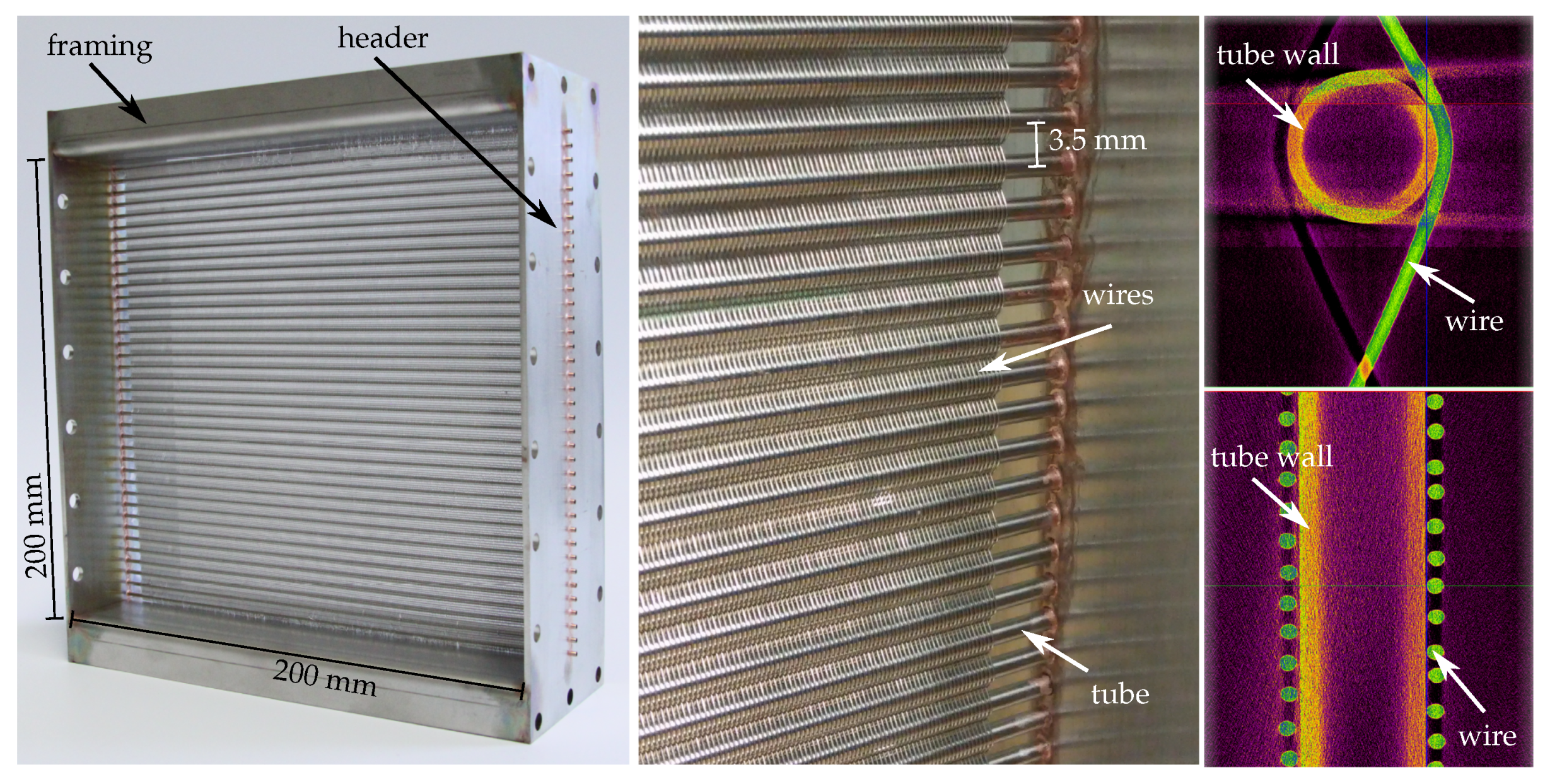
2.1. Test Hardware
2.2. Analysis Model
2.2.1. Governing Equations and Assumptions
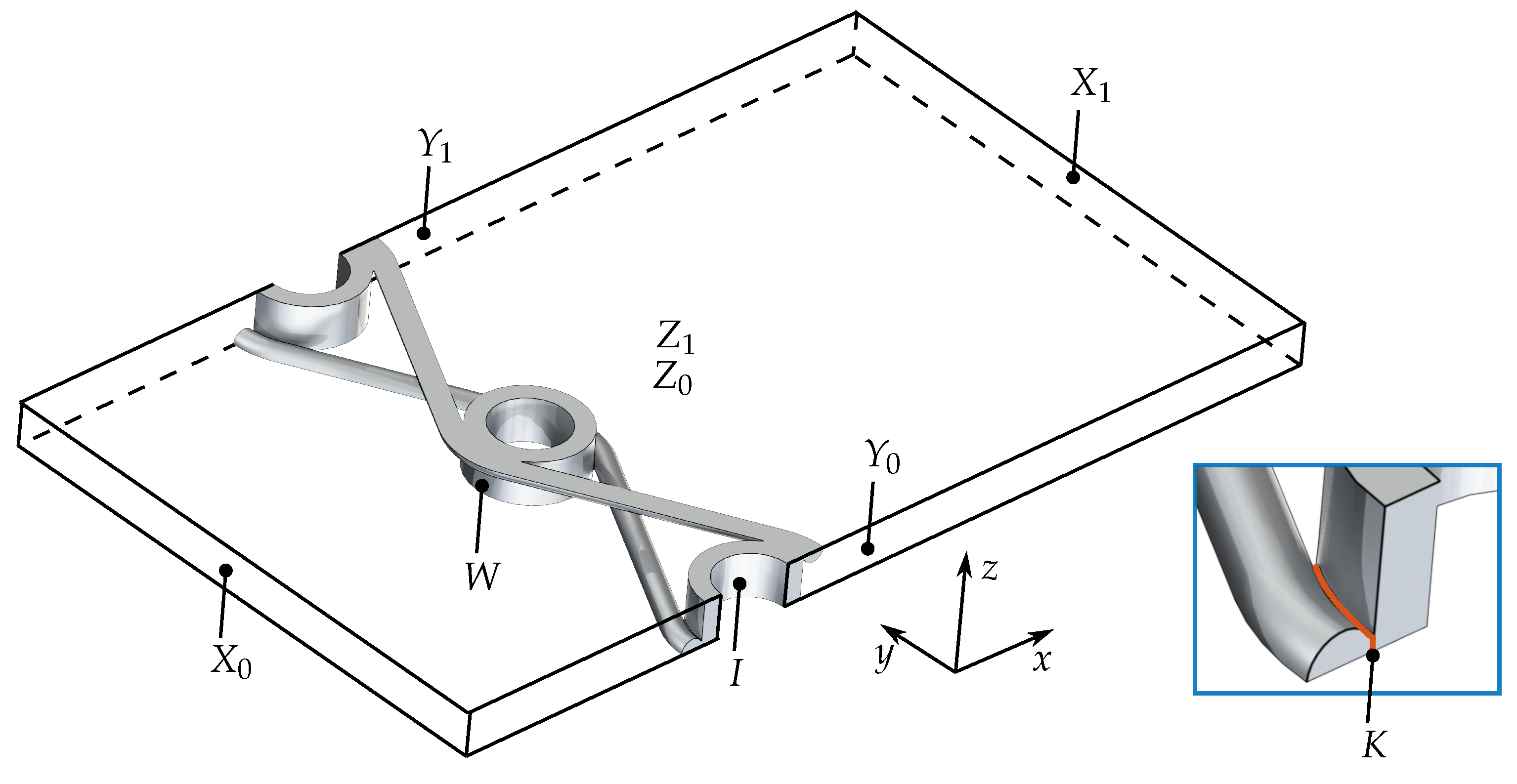
2.2.2. Simulation Domain and Boundary Conditions
2.2.3. One-Way Coupling between Momentum- and Energy-Equation
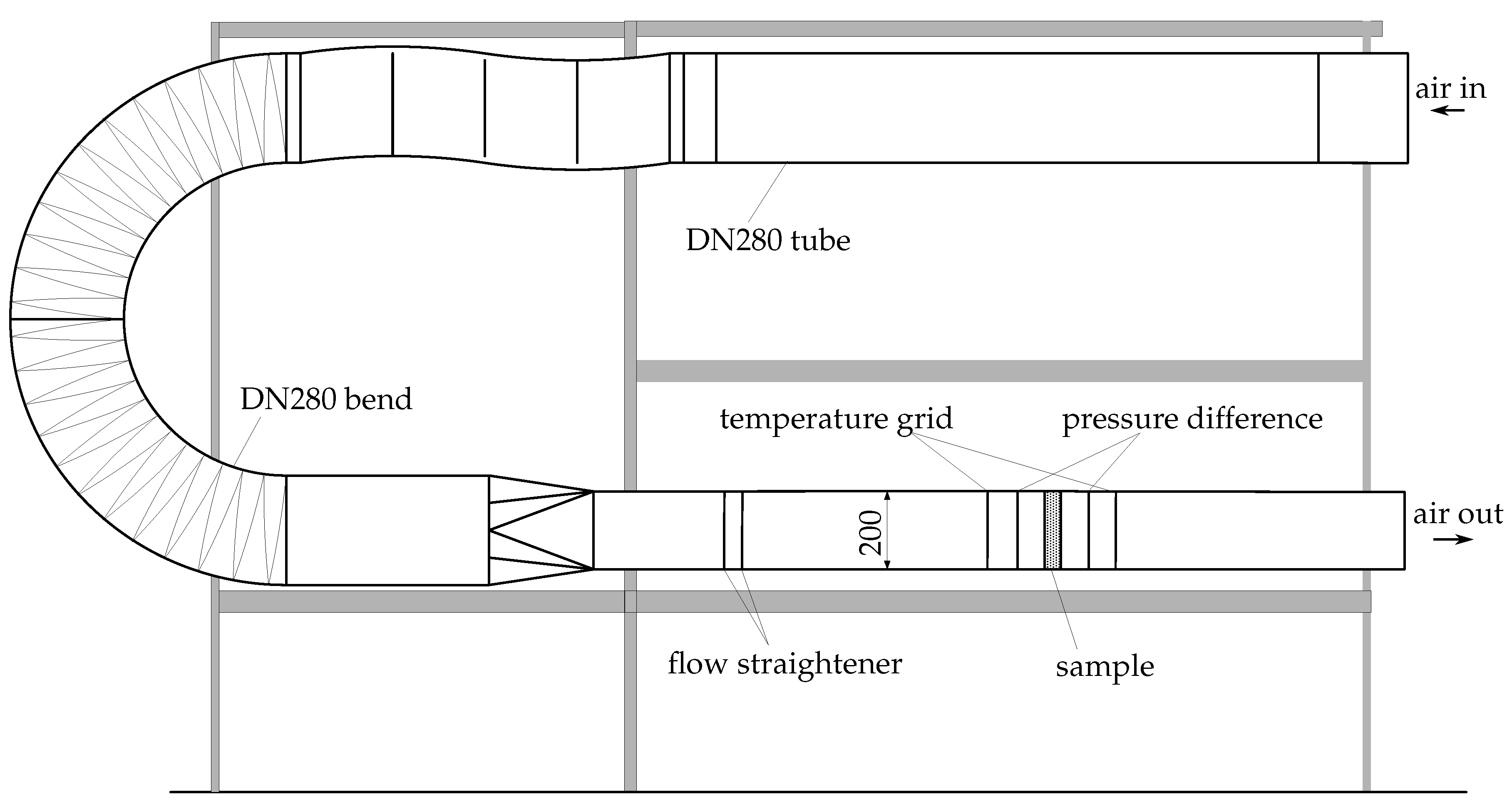
2.3. Experimental Set-Up
2.4. Performance Parameters
3. Results
4. Discussion
5. Conclusions
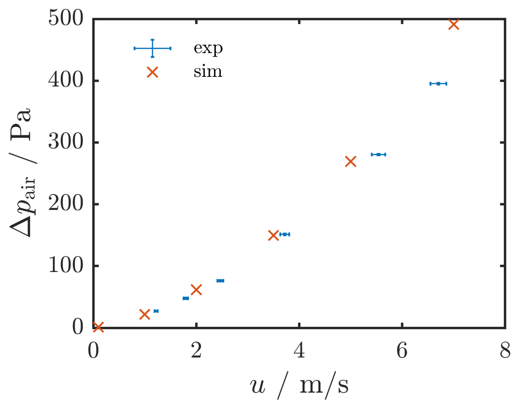
- Simulation results showed reasonable agreement with measured data for pressure drop across the wire cloth with relative differences below 16%.
- The thermal contact between tubes and wires could not be determined independently, thus the thermal contact resistance was fitted with measured data. The fitted value is in good agreement with the values reported in literature.
- Simulated and measured values for the efficient heat transfer coefficient data are in very good agreement based on the fitted thermal contact resistance.
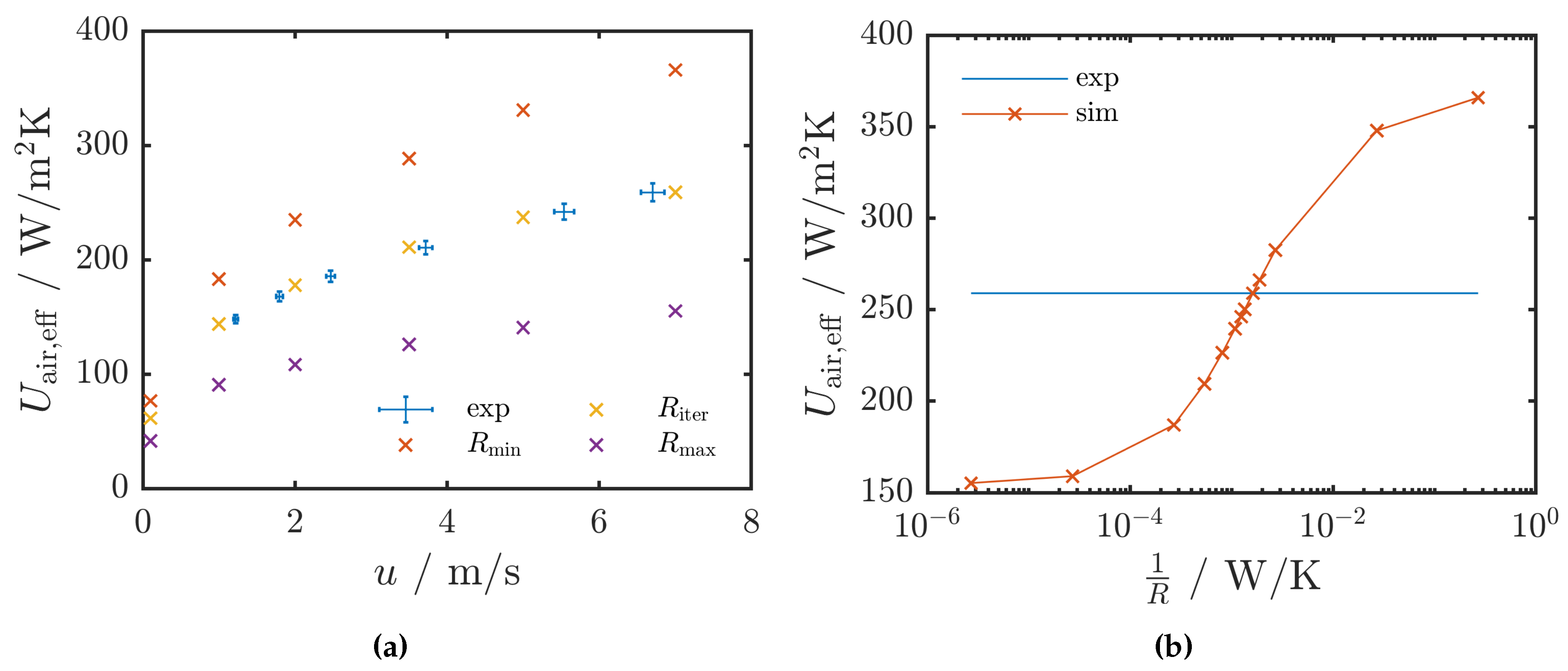
- Values for the efficient heat transfer coefficient are strongly dependent on the thermal contact resistance between tubes and wires. A very good contact could yield up to 40% higher values for the efficient heat transfer coefficient compared to the investigated sample (cf. Figure 7b).
- The produced and tested sample heat exchanger was not intended to yield a good thermal-hydraulic performance, but did allow evaluation of the employed manufacturing wire cloth process and benchmarking of the simulation model. Therefore, the realised performance is only to a limited extent comparable with other types of heat exchangers. Specifically:
- The achieved effective heat transfer coefficient of 180 / at is in the range of very compact louvered fin heat exchangers, but not superior.
- The pressure drop of the wire cloth heat exchanger sample is very high (by a factor of 7 to 11) compared to louvered fin heat exchangers and with respect to the provided heat transfer surface area.
- Wire cloth micro heat exchangers provide flexibility in heat exchanger construction. They allow, for example, curved shapes as well as different spacings of the tubes within one heat exchanger.
Author Contributions
Funding
Acknowledgments
Conflicts of Interest
Abbreviations
| Greek Symbols | |
| heat transfer surface area density (/) | |
| difference of a quantity | |
| angle of contact area tube to wire in y-direction () | |
| angle of contact area tube to wire in z-direction () | |
| efficiency (-) | |
| density () | |
| stress tensor () | |
| temporal standard deviation of the velocity () | |
| Latin Symbols | |
| A | surface area () |
| A | heat transfer surface area of primary and secondary surface on the air-side () |
| heat capacity () | |
| outer tube diameter () | |
| dwall | tube wall thickness () |
| dwire | wire diameter () |
| F | correction factor for flow configuration (-) |
| height of heat exchanger () | |
| h | enthalpy (/) |
| air-side heat transfer coefficient () | |
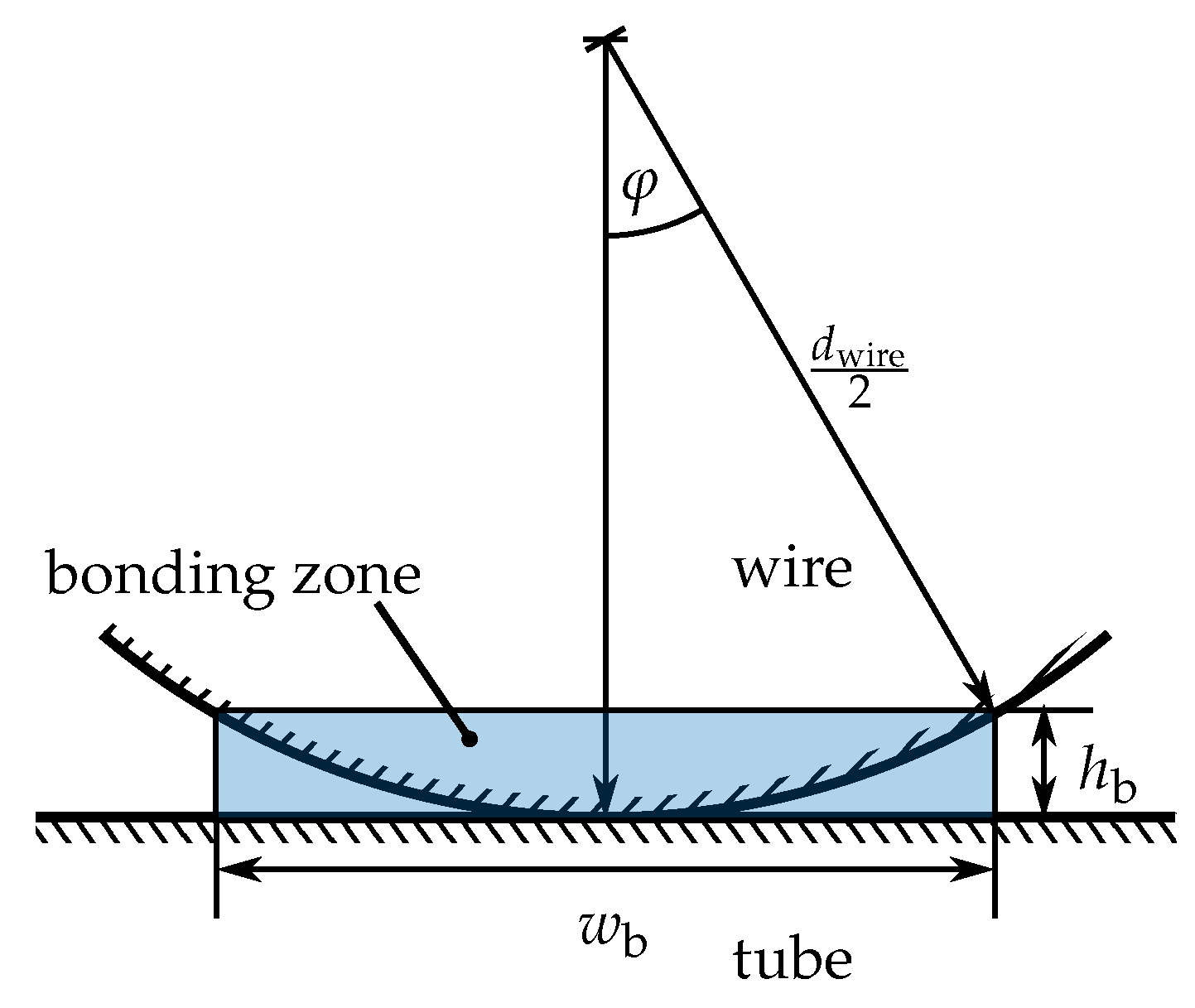
| height of diffusion bonding zone () | |
| water-side heat transfer coefficient () | |
| I | interface between inner tube wall and water |
| K | interface between wire and tube domains |
| k | thermal conductivity () |
| Lst | length of structure () |
| l | length () |
| mass flow rate (/) | |
| number of tubes (-) | |
| normal vector on boundaries () | |
| p | pressure () |
| heat transfer rate within the heat exchanger () | |
| R | thermal resistance () |
| T | temperature () |
| temperature difference () | |
| t | time () |
| wire pitch perpendicular to flow direction () | |
| tube pitch perpendicular to flow direction () | |
| effective heat transfer coefficient () | |
| UHX | overall heat transfer coefficient () |
| u | velocity magnitude () |
| vector for the velocity field () | |
| Volume flow rate () | |
| W | interface between solid and fluid/air domains |
| width of heat exchanger () | |
| w | thickness () |
| X | boundary wall |
| Y | boundary wall |
| Z | boundary wall |
| Subscripts | |
| air | related to the air-side |
| b | bonding zone |
| f | fin |
| HX | heat exchanger |
| in | inlet of the heat exchanger |
| int | interface |
| log | logarithmic mean |
| m | mean |
| out | outlet of the heat exchanger |
| s | related to a straight wire |
| solid | solid domain including wires and tube wall |
| wall | related to the tube wall |
| water | related to the water-side |
| wire | related to the wire |
Appendix A. Geometry Parameters of investigated Wire Cloth

Appendix B. Experimental Information

| Domain | Measured Variable | Technolgy | Range | Standard Uncertainty |
|---|---|---|---|---|
| air | temperature | thin Pt100 | 5–90 | |
| air | volume flow rate | ultrasonic flow meter | 10–270 / | 2% of meas. value |
| air | volume flow rate | orifice plate | 150–1000 / | 2% of meas. value |
| air | pressure drop | differential pressure transmitter | 0–50 | |
| air | pressure drop | differential pressure transmitter | 0–250 | 1 |
| air | absolute pressure | barometric pressure sensor | 500–1100 | |
| water | temperature | Pt100 rod sensor | 5–90 | |
| water | volume flow rate | electromagnetic flow sensor | 0–7.2 / | 0.4% of meas. value |
| water | pressure drop | differential pressure transmitter | 0–0.6 | 3 |
| (/) | (/) | () | () | () | () | () |
|---|---|---|---|---|---|---|
| 169 ± 4 | 0.89 ± 0.004 | 24.5 ± 0.12 | 50.4 ± 0.12 | 84 ± 0.12 | 165.4 ± 0.12 | 54 ± 0.6 |
| 169 ± 4 | 1.08 ± 0.004 | 24.4 ± 0.12 | 50.5 ± 0.12 | 84.1 ± 0.12 | 166 ± 0.12 | 54 ± 0.6 |
| 250 ± 6 | 1.08 ± 0.004 | 24.3 ± 0.12 | 45.6 ± 0.12 | 84.1 ± 0.12 | 165.6 ± 0.12 | 96 ± 1.2 |
| 251 ± 6 | 0.89 ± 0.004 | 24.4 ± 0.12 | 45.4 ± 0.12 | 84 ± 0.12 | 165 ± 0.12 | 96 ± 1.2 |
| 346 ± 8 | 1.08 ± 0.004 | 24.3 ± 0.12 | 42 ± 0.12 | 84.1 ± 0.12 | 165.2 ± 0.12 | 152 ± 1.2 |
| 346 ± 8 | 0.89 ± 0.004 | 24.4 ± 0.12 | 41.9 ± 0.12 | 84 ± 0.12 | 164.4 ± 0.12 | 152 ± 1.2 |
| 526 ± 12 | 1.08 ± 0.004 | 24.4 ± 0.12 | 38.1 ± 0.12 | 84.1 ± 0.12 | 164.6 ± 0.12 | 304 ± 1.2 |
| 526 ± 12 | 0.89 ± 0.004 | 24.5 ± 0.12 | 38.1 ± 0.12 | 84 ± 0.12 | 163.6 ± 0.12 | 302 ± 1.2 |
| 790 ± 18 | 0.89 ± 0.004 | 24.6 ± 0.12 | 35 ± 0.12 | 83.2 ± 0.12 | 161.2 ± 0.12 | 558 ± 1.2 |
| 790 ± 18 | 1.08 ± 0.006 | 24.5 ± 0.12 | 35.3 ± 0.12 | 84.1 ± 0.12 | 163.8 ± 0.12 | 564 ± 1.2 |
| 959 ± 22 | 0.89 ± 0.004 | 24.7 ± 0.12 | 33.6 ± 0.12 | 81.5 ± 0.12 | 157.6 ± 0.12 | 790 ± 1.2 |
| 961 ± 22 | 1.08 ± 0.006 | 24.6 ± 0.12 | 34.1 ± 0.12 | 84.1 ± 0.12 | 163.4 ± 0.12 | 790 ± 1.2 |
References
- Xu, J.; Tian, J.; Lu, T.J.; Hodson, H.P. On the thermal performance of wire-screen meshes as heat exchanger material. Int. J. Heat Mass Transf. 2007, 50, 1141–1154. [Google Scholar] [CrossRef]
- Prasad, S.B.; Saini, J.S.; Singh, K.M. Investigation of heat transfer and friction characteristics of packed bed solar air heater using wire mesh as packing material. Sol. Energy 2009, 83, 773–783. [Google Scholar] [CrossRef]
- Fugmann, H.; Laurenz, E.; Schnabel, L. Wire Structure Heat Exchangers—New Designs for Efficient Heat Transfer. Energies 2017, 10, 1341. [Google Scholar] [CrossRef] [Green Version]
- Liu, Y.; Xu, G.; Luo, X.; Li, H.; Ma, J. An experimental investigation on fluid flow and heat transfer characteristics of sintered woven wire mesh structures. Appl. Therm. Eng. 2015, 80, 118–126. [Google Scholar] [CrossRef]
- Fugmann, H.; Tahir, A.J.; Schnabel, L. Woven Wire Gas-To-Liquid Heat Exchanger. In World Congress on Mechanical, Chemical and Material Engineering; MCM15, Ed.; Avestia Publishing, International ASET Inc.: Ottawa, ON, Canada, 2015. [Google Scholar]
- Fugmann, H.; Di Lauro, P.; Sawant, A.; Schnabel, L. Development of Heat Transfer Surface Area Enhancements: A Test Facility for New Heat Exchanger Designs. Energies 2018, 11, 1322. [Google Scholar] [CrossRef]
- Fugmann, H. Investigation of Wire Structures for Heat Transfer Enhancement in Compact Heat Exchangers. Ph.D. Thesis, Karlsruher Institut für Technologie, Karlsruhe, Germany, 2019. [Google Scholar] [CrossRef]
- Chen, L.; Wirtz, R.A. Development of a high performance heat sink based on screen-fin technology. In Proceedings of the Ninteenth Annual IEEE Semiconductor Thermal Measurement and Management Symposium, San Jose, CA USA, 11–13 March 2003; pp. 53–60. [Google Scholar] [CrossRef]
- van Andel, E.; van Andel, E. Heat Exchanger and Applications Thereof. Patent US7963067 B2, 21 June 2011. [Google Scholar]
- Bonestroo, J.P. Calculation Model of Fine-Wire Heat Exchanger. Master’s Thesis, Twente University, Enschede, The Netherlands, 2012. [Google Scholar]
- Fugmann, H.; Schnabel, L.; Frohnapfel, B. Heat transfer and pressure drop correlations for laminar flow in an in-line and staggered array of circular cylinders. Numer. Heat Transf. Part A Appl. 2019, 75, 1–20. [Google Scholar] [CrossRef]
- Kumra, A.; Rawal, N.; Samui, P. Prediction of Heat Transfer Rate of a Wire-on-Tube Type Heat Exchanger: An Artificial Intelligence Approach. Procedia Eng. 2013, 64, 74–83. [Google Scholar] [CrossRef] [Green Version]
- Lee, T.H.; Yun, J.Y.; Lee, J.S.; Park, J.J.; Lee, K.S. Determination of airside heat transfer coefficient on wire-on-tube type heat exchanger. Int. J. Heat Mass Transf. 2001, 44, 1767–1776. [Google Scholar] [CrossRef]
- van Andel, E. Heat Exchanger and Method for Manufacturing Same. Patent EP0714500 B1, 7 January 1999. [Google Scholar]
- Balzer, R. Wärmetauschvorrichtung für einen Wärmeaustausch zwischen Medien und Webstruktur. Patent DE102006022629, 15 November 2007. [Google Scholar]
- Balzer, R.; Fugmann, H.; Schnabel, L. Wire Cloth Micro Heat Exchanger with High Pressure Stability. In Compact Heat Exchangers: Designs, Materials and Applications; Krüssmann, H., Ed.; PP Publico Publications: Essen, Germany, 2018. [Google Scholar]
- Radermacher, R.; Bacellar, D.; Aute, V.; Huang, Z.; Hwang, Y.; Ling, J.; Muehlbauer, J.; Tancabel, J.; Abdelaziz, O.; Zhang, M. Miniaturized Air-to-Refrigerant Heat Exchangers; University of Maryland: College Park, MD, USA, 2017. [Google Scholar] [CrossRef]
- VDI. VDI-Wärmeatlas; Springer: Berlin, Germany, 2013. [Google Scholar]
- Martens, S. Modellierung und numerische Berechnung der thermofluiddynamischen Eigenschaften gewebebasierter Wärmeübertrager. Ph.D. Thesis, Universität Stuttgart, Stuttgart, Germany, 2019. [Google Scholar]
- Shah, R.K.; Sekulić, D.P. Fundamentals of Heat Exchanger Design; Wiley: Hoboken, NJ, USA, 2003. [Google Scholar]
- Nicholas, M.G.; Crispin, R.M. Diffusion bonding stainless steel to alumina using aluminium interlayers. J. Mater. Sci. 1982, 17, 3347–3360. [Google Scholar] [CrossRef]
- Mahendran, G.; Balasubramanian, V.; Senthilvelan, T. Influences of diffusion bonding process parameters on bond characteristics of Mg-Cu dissimilar joints. Trans. Nonferrous Met. Soc. China 2010, 20, 997–1005. [Google Scholar] [CrossRef]
- Nakaso, K.; Mitani, H.; Fukai, J. Convection heat transfer in a shell-and-tube heat exchanger using sheet fins for effective utilization of energy. Int. J. Heat Mass Transf. 2015, 82, 581–587. [Google Scholar] [CrossRef]
- Yovanovich, M.M.; Tuarze, M. Experimental Evidence of Thermal Resistance at Soldered Joints. J. Spacecr. Rockets 1969, 6, 855–857. [Google Scholar] [CrossRef]


| Specification | Parameter | Unit | Wire Structure |
|---|---|---|---|
| material | - | - | stainless steel |
| thermal conductivity | ksolid | /() | 20 |
| number of tubes | - | 57 | |
| width of heat exchanger | 200 | ||
| height of heat exchanger | 200 | ||
| length of structure in flow direction | 2.4 | ||
| outer diameter tubes | 2 | ||
| tube wall thickness | 0.2 | ||
| tube pitch perpendicular to flow direction | 3.5 | ||
| wire diameter | d | 200 | |
| wire pitch perpendicular to flow direction | 200 | ||
| heat transfer surface area | AHTS | 0.2227 | |
| heat transfer surface area density | / | 2320 |
| # | Domain | Coupled? | ||
|---|---|---|---|---|
| ref. | large | yes | - | - |
| 1 | large | no | 5.3% | |
| 2 | small | yes | 3.6% | −2.2% |
| 3 | small | no | 3.6% | −2.1% |
© 2020 by the authors. Licensee MDPI, Basel, Switzerland. This article is an open access article distributed under the terms and conditions of the Creative Commons Attribution (CC BY) license (http://creativecommons.org/licenses/by/4.0/).
Share and Cite
Fugmann, H.; Martens, S.; Balzer, R.; Brenner, M.; Schnabel, L.; Mehring, C. Performance Evaluation of Wire Cloth Micro Heat Exchangers. Energies 2020, 13, 715. https://doi.org/10.3390/en13030715
Fugmann H, Martens S, Balzer R, Brenner M, Schnabel L, Mehring C. Performance Evaluation of Wire Cloth Micro Heat Exchangers. Energies. 2020; 13(3):715. https://doi.org/10.3390/en13030715
Chicago/Turabian StyleFugmann, Hannes, Sebastian Martens, Richard Balzer, Martin Brenner, Lena Schnabel, and Carsten Mehring. 2020. "Performance Evaluation of Wire Cloth Micro Heat Exchangers" Energies 13, no. 3: 715. https://doi.org/10.3390/en13030715