Optimal Operation for Integrated Electricity–Heat System with Improved Heat Pump and Storage Model to Enhance Local Energy Utilization


Abstract
:1. Introduction
- The nonlinear characteristics of the energy conversion units are addressed. For modeling heat pumps, the relationship of heat production and power consumption is expressed by a quadratic function and transformed to conic constraints by the second-order conic relaxation. Additionally, a new expression of stratified heat storage water tank is proposed to be incorporated in the proposed network model.
- A network constrained optimal operation model for the integrated power and heat system is then proposed based on mixed-integer second-order conic programming (MISOCP). For the operation of PDN, ACOPF is modeled and described by the branch flow model. For the operation of DHN, a convex description of the thermal network based on conic relaxation is applied, in which water flow could be adjusted in different time slots while considering temperature dynamics.
- For a decentralized operation between thermal network and electricity network without a centralized operator, an ADMM based approach is proposed to reconstruct the centralized co-operation model into separated network models run by independent heat system operator (HSO) and distribution system operator (DSO). In the proposed structure for decentralized optimization, HSO and DSO can independently operate DHN and PDN with limited information exchange. As shown by the numerical study, a near-optimal solution could be found through iterations, which is very close to the centralized optimization result.
2. Preliminaries and Notations
2.1. Integrated Electricity and Heat System
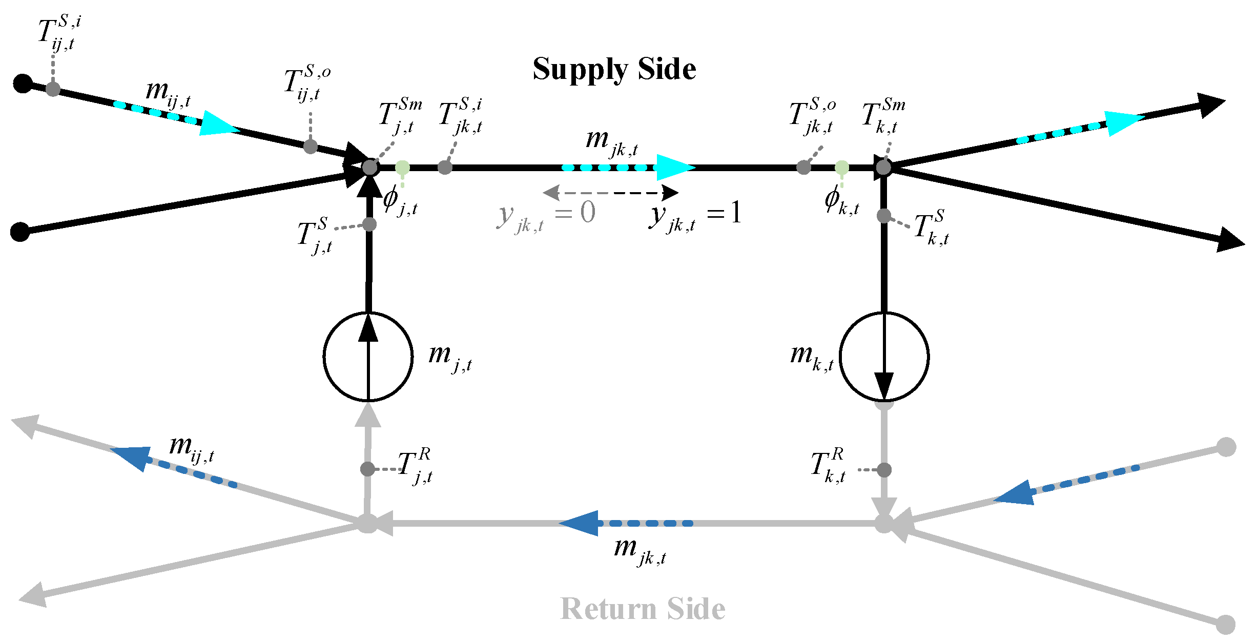
2.2. Notations of District Heating Network
2.3. Notations of Power Distribution Network
3. Problem Formulation
3.1. Objective
3.2. Constraints
3.2.1. Component Constraints
- Combined Heat and Power
- Heat pumps
- PV units
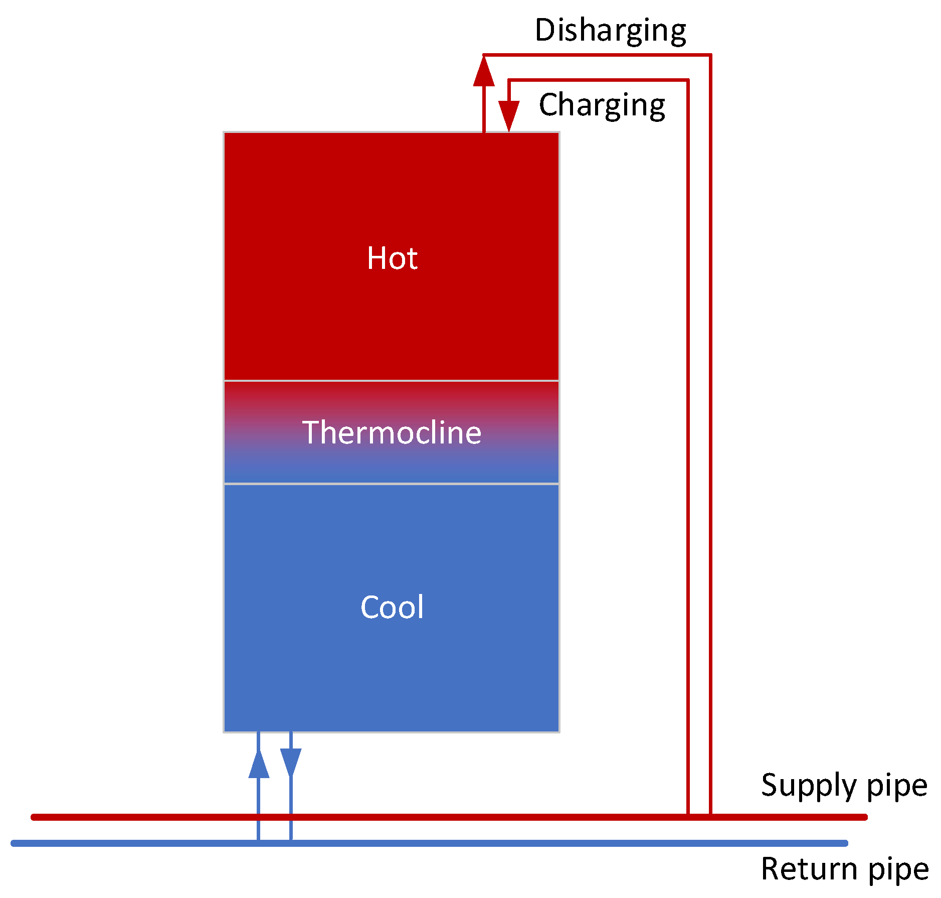
- Heat Storage
3.2.2. Operation Constraints of DHN Model
3.2.3. Operation Constraints of PDN Model
4. Solution Technology
4.1. Convexification of Our Proposed Operation Model
- Heat and its Balance
- Pressure Loss
- Heat Loss
- Temperature Mixing
4.2. ADMM-Based Decentralized Operation
5. Simulation and Results
5.1. System Configuration
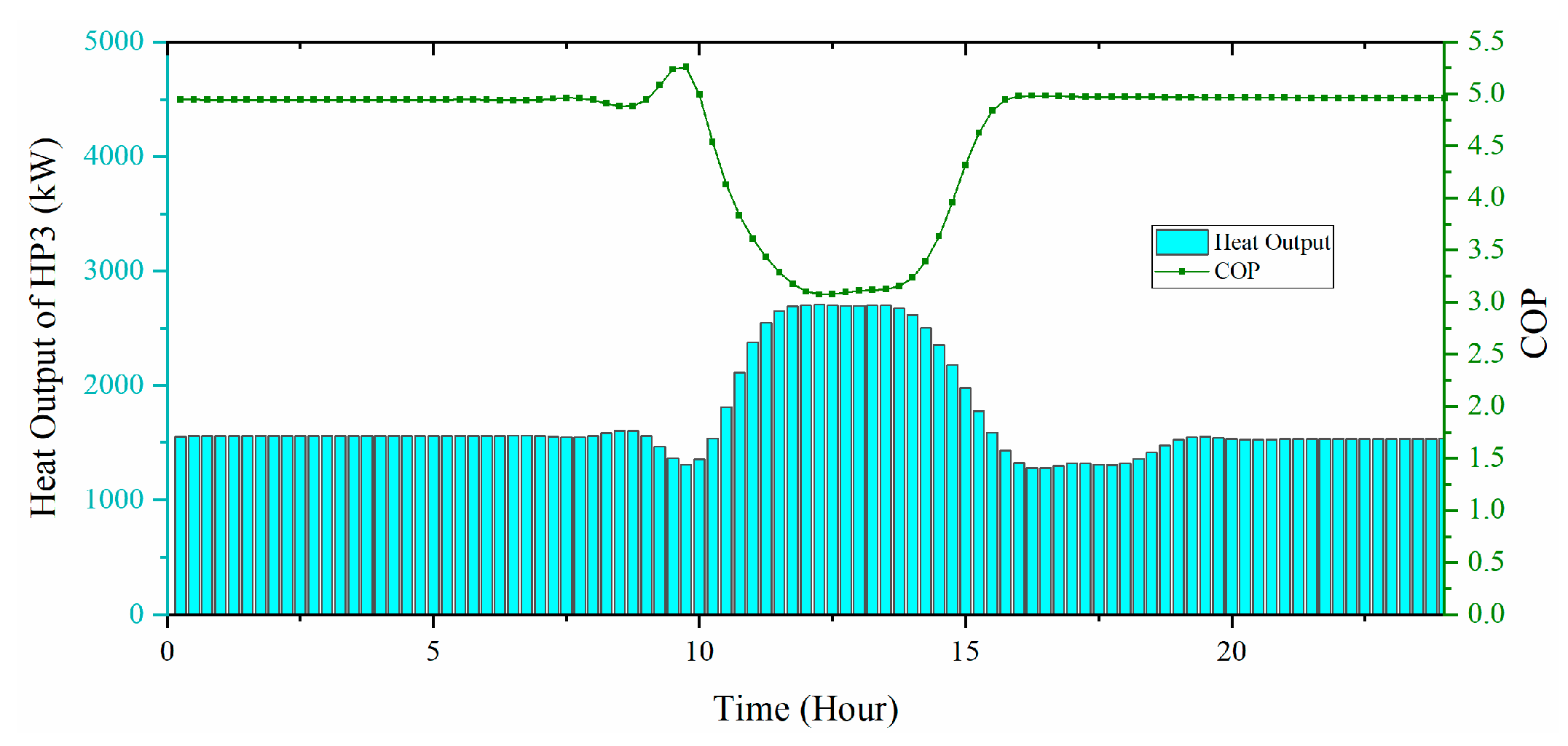
5.2. Optimal Results of DHN-PDN Co-Operation
5.3. Comparison of Different Operation Models
- Case I: Proposed Co-Operation of PDN and DHN (CO)
- Case II: Decoupled Operation of PDN and DHN (DO)
6. Discussion
6.1. Rationality of Assumptions in the Network Model
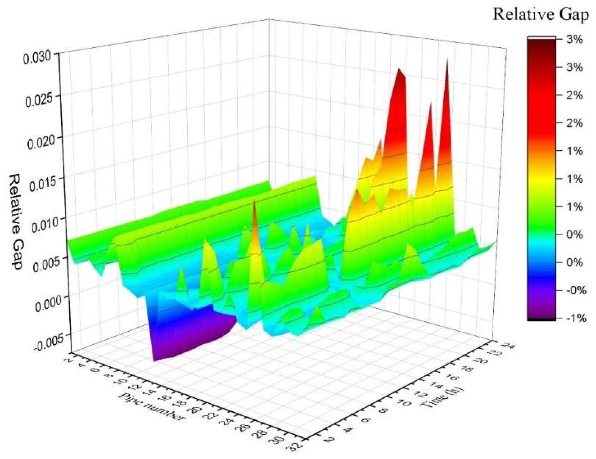
6.2. Exactness of MISOCP in Proposed Model
7. Conclusions
- The proposed model could generate solutions with high accuracy and optimality. On one hand, precise models for both electricity and thermal networks are adopted. Particularly, the VFVT DHN model provides more flexibility than models with the mass flows fixed without loss of accuracy. On the other hand, improved descriptions on heat pumps with variable COP as well as the stratified water tank for heat storage are included and reformulated to integrate with the network model, making the proposed model closer to the actual situation.
- Flexibility of the electricity distribution system could be enhanced through the co-operation of integrated energy system. As a result, the co-operation model of an integrated system could facilitate local energy accommodation and reduce the total operation cost. Compared to the DO, CO’s total operation cost is lower by 2.3% to 4.4% under different scenarios. Additionally, results show that the grid supply electricity is about 149.1MWh per day in DO, 23% larger than 121.4 MWh in CO.
- Decentralized optimization based on ADMM could provide a near-optimal solution but with little sharing of private information. With the distributed techniques, the co-operation could be achieved in a decentralized way with little loss of efficiency. Due to the nonconvexity of MISOCP, there would be a rather small gap (≤0.1%) between the decentralized case with the centralized one. Nevertheless, the operation costs in both cases are significantly decreased compared to the decoupled operation of DHN and PDN.
Supplementary Materials
Author Contributions
Funding
Conflicts of Interest
Nomenclature
| , | Indices of sending and receiving buses of the PDN |
| Indices of sending and receiving nodes of the DHN | |
| Indices of all Heat and Power market participants (Generation/Demands) | |
| Index for times of iteration | |
| Indices of time periods | |
| Set of buses in the PDN | |
| Set of buses in the DHN | |
| Sets of source nodes in the DHN | |
| Sets of demand nodes in the DHN | |
| Sets of storage nodes in the DHN | |
| Set of heat pump systems | |
| Set of time periods | |
| Sets of buses in PDN with heat pump system located | |
| Sets of nodes in DHN with heat pump system located | |
| Sets of Ancestor/Child nodes of node | |
| Specific heat capacity of water | |
| Static active and reactive demand at bus at time | |
| Energy conversion parameters of heat pump in HP system | |
| Power consumption/output capacity of heat pump system | |
| heat production capacity of heat pump | |
| Maximal charging/discharging heat of thermal storage | |
| Storage tank capacity (in heat) of thermal storage | |
| Temperature difference between supply and return network of DHN at node | |
| Upper and lower bounds of temperature in supply network of DHN | |
| Upper and lower bounds of temperature in supply network of DHN | |
| Heat conductance of pipeline from node to node | |
| Upper bound of squared voltage at bus | |
| Upper bound of squared current from bus to | |
| Heat loss in the storage tank | |
| Charging/discharging efficiency of thermal storage | |
| Predicted injection mass flow rate from node to node in supply network | |
| Predicted injection mass flow rate from node to node in return network | |
| Predicted injection/outlet mass flow rate at node | |
| Resistance/reactance from bus to | |
| Price for grid supply heat at time | |
| Coefficient of pressure-mass flow formula in heat pipe | |
| / | Heat loss in heat pipe of supply/return network at time |
| Offer price of heat pump system at time in Electricity Market | |
| Bid price of heat pump system at time in Electricity Market | |
| Offer price of heat pump system at time in Heat Market | |
| Heat output of heat pump at time | |
| Power consumption of heat pump at time | |
| Discharging heat rate of storage at time | |
| Charging heat rate of storage at time | |
| Heat loss of storage at time | |
| Stored thermal energy of storage in system at time | |
| Accumulated heat loss of storage in system at time | |
| Binary variables for storage in system at time indicating loss | |
| Heat supply from traditional generator at time | |
| Flexible demand at time t | |
| Mass flow rate from node to at time | |
| Mass flow rate injected to node at time | |
| Water Pressure at node | |
| Pressure loss along the pipe from node to at time | |
| Temperature at node in the supply network | |
| Temperature at node in the return network | |
| Mixed temperature at node in the supply network | |
| Mixed temperature at node in the return network | |
| Temperature at the inlet port of pipe from node to at time in the supply network | |
| Temperature at the outlet port of pipe from node to at time in the supply network | |
| Temperature at the inlet port of pipe from node to at time in the return network | |
| Temperature at the outlet port of pipe from node to at time in the return network | |
| Temperature loss along the pipe in the supply network from node to at time | |
| Temperature loss along the pipe in the return network from node to at time | |
| Active power generation/demand at time | |
| Primal objective of heating market | |
| Reactive power generation/demand at time | |
| Active power flow in the branch from bus to at time | |
| Reactive power flow in the branch from bus to at time | |
| Squared voltage at bus at time | |
| Squared current from bus to at time | |
| Dual variable | |
| Dual variable |
References
- Grid-Connected Operation of Photovoltaic Power Generation in 2019. Available online: http://www.nea.gov.cn/2020-02/28/c_138827923.htm/ (accessed on 18 November 2020).
- Mazidi, P.; Baltas, G.N.; Eliassi, M.; Rodriguez, P.; Pastor, R.; Michael, M.; Tapakis, R.; Vita, V.; Zafiropoulos, E.; Dikeakos, C. Zero Renewable Incentive Analysis for Flexibility Study of a Grid. In Proceedings of the International Symposium on High Voltage Engineering, Budapest, Hungary, 26–30 August 2019; pp. 47–60. [Google Scholar]
- Levelized Cost of Energy and Levelized Cost of Storage. 2020. Available online: https://www.lazard.com/perspective/levelized-cost-of-energy-and-levelized-cost-of-storage-2020/ (accessed on 18 November 2020).
- Zhang, M.; Wu, Q.; Wen, J.; Lin, Z.; Chen, Q. Optimal operation of integrated electricity and heat system: A review of modeling and solution methods. Renew. Sustain. Energy Rev. 2020, 135, 110098. [Google Scholar] [CrossRef]
- Bilgen, E.; Takahashi, H. Exergy analysis and experimental study of heat pump systems. Exergy 2002, 2, 259–265. [Google Scholar] [CrossRef]
- A Review of Domestic Heat Pump Coefficient of Performance; Birmingham University. 2009. Available online: https://www.academia.edu/1073992/A_review_of_domestic_heat_pump_coefficient_of_performance (accessed on 15 October 2020).
- Cao, Y.; Wei, W.; Wu, L.; Mei, S.; Shahidehpour, M.; Li, Z. Decentralized Operation of Interdependent Power Distribution Network and District Heating Network: A Market-Driven Approach. IEEE Trans. Smart Grid 2019, 10, 5374–5385. [Google Scholar] [CrossRef]
- Soomro, A.A.; Mokhtar, A.A.; Akbar, A.; Abbasi, A. Modelling Techniques Used in the Analysis of Stratified Thermal Energy Storage: A Review. Proc. MATEC Web Conf. 2018. [Google Scholar] [CrossRef]
- Chen, X.; Kang, C.; O’Malley, M.; Xia, Q.; Bai, J.; Liu, C.; Sun, R.; Wang, W.; Li, H. Increasing the Flexibility of Combined Heat and Power for Wind Power Integration in China: Modeling and Implications. IEEE Trans. Power Syst. 2015, 30, 1848–1857. [Google Scholar] [CrossRef]
- Tyagi, V.V.; Buddhi, D. PCM thermal storage in buildings: A state of art. Renew. Sustain. Energy Rev. 2007, 11, 1146–1166. [Google Scholar] [CrossRef]
- Tao, G.; Henwood, M.I.; Ooijen, M.V. An algorithm for combined heat and power economic dispatch. IEEE Trans. Power Syst. 1996, 11, 1778–1784. [Google Scholar] [CrossRef]
- Belli, G.; Giordano, A.; Mastroianni, C.; Menniti, D.; Pinnarelli, A.; Scarcello, L.; Sorrentino, N.; Stillo, M. A Unified Model for the Optimal Management of Electrical and Thermal Equipment of a Prosumer in a DR Environment. IEEE Trans. Smart Grid 2017, 10, 1791–1800. [Google Scholar] [CrossRef]
- Purchala, K.; Meeus, L.; Van Dommelen, D.; Belmans, R. Usefulness of DC power flow for active power flow analysis. In Proceedings of the IEEE Power Engineering Society General Meeting, Denver, CO, USA, 26–30 July 2005; pp. 454–459. [Google Scholar]
- Bai, X.Q.; Wei, H.; Fujisawa, K.; Wang, Y. Semidefinite programming for optimal power flow problems. Int. J. Electr. Power 2008, 30, 383–392. [Google Scholar] [CrossRef]
- Lavaei, J. Zero duality gap for classical OPF problem convexifies fundamental nonlinear power problems. In Proceedings of the 2011 American Control Conference, San Francisco, CA, USA, 29 June–1 July 2011; pp. 4566–4573. [Google Scholar]
- Farivar, M.; Low, S.H. Branch Flow Model: Relaxations and Convexification—Part I. IEEE Trans. Power Syst. 2013, 28, 2565–2572. [Google Scholar] [CrossRef]
- Liu, X.Z.; Wu, J.Z.; Jenkins, N.; Bagdanavicius, A. Combined analysis of electricity and heat networks. Appl. Energy 2016, 162, 1238–1250. [Google Scholar] [CrossRef] [Green Version]
- Li, Z.; Wu, W.; Shahidehpour, M.; Wang, J.; Zhang, B. Combined Heat and Power Dispatch Considering Pipeline Energy Storage of District Heating Network. IEEE Trans. Sustain. Energy 2015, 7, 12–22. [Google Scholar] [CrossRef]
- Wang, D.; Zhi, Y.Q.; Jia, H.J.; Hou, K.; Zhang, S.X.; Du, W.; Wang, X.D.; Fan, M.H. Optimal scheduling strategy of district integrated heat and power system with wind power and multiple energy stations considering thermal inertia of buildings under different heating regulation modes. Appl. Energy 2019, 240, 341–358. [Google Scholar] [CrossRef]
- Li, Z.; Wu, W.; Wang, J.; Zhang, B.; Zheng, T. Transmission-Constrained Unit Commitment Considering Combined Electricity and District Heating Networks. IEEE Trans. Sustain. Energy 2016, 7, 480–492. [Google Scholar] [CrossRef]
- Jiang, Y.; Wan, C.; Botterud, A.; Song, Y.; Shahidehpour, M. Convex Relaxation of Combined Heat and Power Dispatch. IEEE Trans. Power Syst. 2020. [Google Scholar] [CrossRef]
- Huang, S.; Tang, W.; Wu, Q.; Li, C. Network constrained economic dispatch of integrated heat and electricity systems through mixed integer conic programming. Energy 2019, 179, 464–474. [Google Scholar] [CrossRef] [Green Version]
- Kar, S.; Hug, G. Distributed robust economic dispatch in power systems: A consensus + innovations approach. In Proceedings of the Power and Energy Society General Meeting, San Diego, CA, USA, 22–26 July 2012. [Google Scholar]
- Sorin, E.; Bobo, L.; Pinson, P. Consensus-based approach to peer-to-peer electricity markets with product differentiation. IEEE Trans. Power Syst. 2018, 34, 994–1004. [Google Scholar] [CrossRef] [Green Version]
- Shen, F.; López, J.C.; Wu, Q.; Rider, M.J.; Lu, T.; Hatziargyriou, N.D. Distributed Self-Healing Scheme for Unbalanced Electrical Distribution Systems Based on Alternating Direction Method of Multipliers. IEEE Trans. Power Syst. 2020, 35, 2190–2199. [Google Scholar] [CrossRef]
- Li, J.; Zhang, C.; Zhao, X.; Wang, J.; Jian, Z.; Zhang, Y.-J.A. Distributed Transactive Energy Trading Framework in Distribution Networks. IEEE Trans. Power Syst. 2018, 33, 7215–7227. [Google Scholar] [CrossRef]


| Scenario | Case II: CO | Case II: DO | CR Ratio | ||
|---|---|---|---|---|---|
| Total Cost (kRMB/d) | Cost (kRMB/d) | ||||
| PDN | DHN | Total | |||
| S1 | 102.96 | 85.597 | 19.824 | 105.42 | 2.30% |
| S2 | 94.826 | 78.418 | 19.824 | 98.242 | 3.60% |
| S3 | 94.755 | 78.413 | 19.824 | 98.237 | 3.70% |
| S4 | 92.900 | 77.171 | 19.824 | 96.995 | 4.40% |
| Case | Maximal Gap | ||
|---|---|---|---|
| Pressure Loss | Heat Loss | Heat Pump COP | |
| with penalty () | 0.0063 | 0.0016 | 2.69 × 10⁻⁷ |
| w/o penalty | 7964.8 | 53.88 | 1.30 × 10⁻⁶ |
Publisher’s Note: MDPI stays neutral with regard to jurisdictional claims in published maps and institutional affiliations. |
© 2020 by the authors. Licensee MDPI, Basel, Switzerland. This article is an open access article distributed under the terms and conditions of the Creative Commons Attribution (CC BY) license (http://creativecommons.org/licenses/by/4.0/).
Share and Cite
Chen, Y.; Zhang, Y.; Wang, J.; Lu, Z. Optimal Operation for Integrated Electricity–Heat System with Improved Heat Pump and Storage Model to Enhance Local Energy Utilization. Energies 2020, 13, 6729. https://doi.org/10.3390/en13246729
Chen Y, Zhang Y, Wang J, Lu Z. Optimal Operation for Integrated Electricity–Heat System with Improved Heat Pump and Storage Model to Enhance Local Energy Utilization. Energies. 2020; 13(24):6729. https://doi.org/10.3390/en13246729
Chicago/Turabian StyleChen, Yang, Yao Zhang, Jianxue Wang, and Zelong Lu. 2020. "Optimal Operation for Integrated Electricity–Heat System with Improved Heat Pump and Storage Model to Enhance Local Energy Utilization" Energies 13, no. 24: 6729. https://doi.org/10.3390/en13246729