Numerical and Experimental Analysis of Heat Transfer for Solid Fuels Combustion in Fixed Bed Conditions


Department of Fuels and Renewable Energy, Faculty of Environmental Engineering and Energy, Institute of Thermal Engineering, Poznan University of Technology, 60-965 Poznan, Poland
Energies 2020, 13(22), 6141; https://doi.org/10.3390/en13226141
Submission received: 11 November 2020
/
Revised: 19 November 2020
/
Accepted: 20 November 2020
/
Published: 23 November 2020
(This article belongs to the Special Issue Computational Thermal, Energy, and Environmental Engineering)
Abstract
:The paper concerns the analysis of the heat transfer process that occurred during solid fuel burning in fixed bed conditions. The subject of the analysis is a cylindrical combustion chamber with an output of 12 kW heating power equipped with a retort burner for hard coal and biomass combustion. During the research, a numerical and experimental study is performed. The analysis is prepared for various heat load of the combustion chamber, which allowed for the reconstruction of real working conditions for heating devices working with solid fuels combustion. The temperature distribution obtained by the experimental way is compared with results of the numerical modeling. Local distribution of principal heat transfer magnitudes like a heat flux density and a heat transfer coefficient that occurred on the sidewall of the combustion chamber is analyzed. The analysis showed, that the participation of convection and radiation in the overall heat transfer process has resulted from the heat load of the heating device. Research results may be used for improving an analytical approach of design process taking place for domestic and industrial combustion chambers.
Keywords:
solid fuels; fixed bed; combustion; heat transfer; heat load; CFD; modeling; experimental analysis1. Introduction
Solid fuel combustion is one of the main sources of thermal energy used for heating purposes by the individual and commercial sector in Poland. According to data from 2018 [1], 35.7% of Polish households were heated by heating devices using solid fuels. Heat provided by thermal plants was delivered to 40.4% of Polish households. The Energy Regulatory Office in Poland reported [2] that in 2019 solid fuel combustion was responsible for 80.2% of the heat generated by the commercial sector. Moreover, 9.2% of the heat generated by the commercial sector originated from solid biomass burning. Nowadays changes in thinking about the environment cause the replacement of fossil fuel by renewable fuels like biomass. From one year to another the amount of heat generated by fossil fuel burning decreases and is replaced by different types of renewable sources of energy. Solid biomass share in energy production from renewable sources in Poland was equal to 67.9% in 2017. European Union average for the mentioned magnitude was 42% in the same year [3]. This means that solid fuel burning for some time will be still the main source of heat generation.
One of the main methods for solid fuel combustion for domestic and industrial boilers is realized in fixed bed conditions. Computational Fluid Dynamic (CFD) modeling is often used to simulate packed bed burning. Fixed bed combustion modeling can be divided into two main groups. The first group is concerned with a small-scale, when a combustion process is realized in a range of heating power equal from over a dozen to tens of kilowatts. The mentioned group may belong to one-dimensional models focused on the phenomena that occurred during combustion of a single grain of a fuel. The second one deals with a huge scale, where obtained heating power from fixed bed combustion equals from few to tens megawatts.
Scharler et al. [4] raised the issue of how the low power log stove burning modeling focused on CO concentration in the flue gas. Wiese et al. [5] have been dealing with a transient simulation of pellet burning with the application of a discrete element model in CFD calculations for a 13 kW stove. Mehrabian et al. [6] and Gomez et al. [7] are concerned with numerical modeling of the thermally thick approach of biomass burning. Gomez et al. [8] also have been using the mentioned approach for a 27 kW domestic boiler working conditions modeling. In other works [9,10] he also modeled emissions of harmful compounds during fixed-bed biomass burning in a 60 kW domestic boiler by steady and transient analysis. Similar transient modeling connected with the analysis of the chemical composition of exhausts was realized by Mehrabian et al. [11] in a laboratory-scale biomass fixed bed batch. Collazo et al. [12] also have been working on a transient simulation of a pellet wood burning for a laboratory combustor. He was targeting a temperature distribution at different points in the bed. Researchers from Clausthal University of Technology and Silesian University of Technology [13,14] were involved in numerical modeling of coal burning in small-scale retort boilers. They analyzed possibilities of the perfecting of domestic boiler construction in terms of pollution limitation and optimization of temperature distribution inside a combustion chamber. Chaney et al. [15] modeled a 50 kw packed bed biomass boiler in terms of investigating the optimization of the combustion performance and NOx emissions. A new approach of packed bed biomass burning was presented by Chapela et al. [16]. His Eulerian-fouling model is computationally less expensive and shows a better response to the experimental data.
Tu et al. [17,18] modeled a 32 MW woodchip-fired grate boiler work with different operating conditions directed on NOx reduction mechanisms. Silva et al. [19] were concerned about 34.6 MW biomass grate-fired boiler modeling. He was focused on an analysis of temperature, velocity, and species field of exhaust gas within a boiler, which provided to the optimization of the burning process. Moving grate biomass boilers models realized in two different scales (250 kW and 4 MW) were analyzed by Rezeau et al. [20] and Bermúdez et al. [21] in terms of composition and temperature distribution of flue gas. Klason et al. [22] analyzed a radiation heat transfer process in two various scales (10 kW and 50 MW) during biomass burning in fixed bed furnaces. He has obtained a gas temperature profile inside the combustion chamber located above a fixed bed with the assumption of constant temperature for furnace walls. Moreover, he investigated the accuracy of a solution for different radiation heat transfer models.
The abovementioned research connected with the fixed bed modeling is concerned mainly with the emission of harmful compounds during solid fuel combustion. Moreover, there has been raised the issue of the temperature distribution occurring in the combustion chamber and inside a packed bed of fuel. Researchers do not relate achieved results of temperature distribution to prepare an in-depth analysis of the heat transfer process in modeled heating devices. The issue of heat transfer phenomenon occurring in a wall neighborhood and free-room of a combustion chamber during fixed-bed combustion still has not been deeply recognized like it is realized in other types of thermal devices used for different industrial applications, like heat treatment furnaces [23,24,25], heat storage systems [26,27,28], or heat exchangers [29,30,31]. So far available results concerned about the packed bed burning assumed a temperature of combustion chamber walls as a boundary condition. Then a constant wall temperature was present for each wall of the combustion chamber or separately, at particular elements of modeled furnaces. Computational grids used in computational models were suitable for free-room analysis like bulk gas temperature and chemical composition. Grids used in the previous research were not capable of heat transfer analysis that occurred on combustion chamber walls. This was caused by the size of grid elements located near the combustion chamber wall (dimensionless wall distance y+ >>1) being too high to obtain an appropriate solution of heat flux at the wall of the combustion chamber. Moreover, so far available packed bed burning models used wall functions for simulating the near-wall region (k-ε model of turbulence). The mentioned approach does not show sufficient accuracy for viable modeling of conditions that occurred near combustion chamber walls which are necessary for modeling a heat transfer process.
2. Materials and Methods
2.1. Initial Assumptions
The author analyzed a case when a combustion process has occurred inside fixed bed conditions. Conducted research was divided into two main parts. Firstly, an experimental analysis was prepared. The second part has relied on the preparation of a numerical model. The combustion process of two types of solid fuels was analyzed. It was hard coal and wood biomass in a pellet form. Proximate and ultimate analysis of fuels used during the research is presented in Table 1. The author analyzed the work of the test stand with two levels of heating power. It was 50% and 100% of the nominal heat load. The test stand used during the conducted research is capable of transferring 12 kW of heat to the cooling water during nominal work. The proposed research is concerned with the investigation of the heat transfer phenomenon that occurred in a near-wall region of the combustion chamber. Application of various types of fuels and levels of a heat load allowed for an analysis occurring during real exploitation in the whole range of heating device working conditions.
2.2. Experimental Research
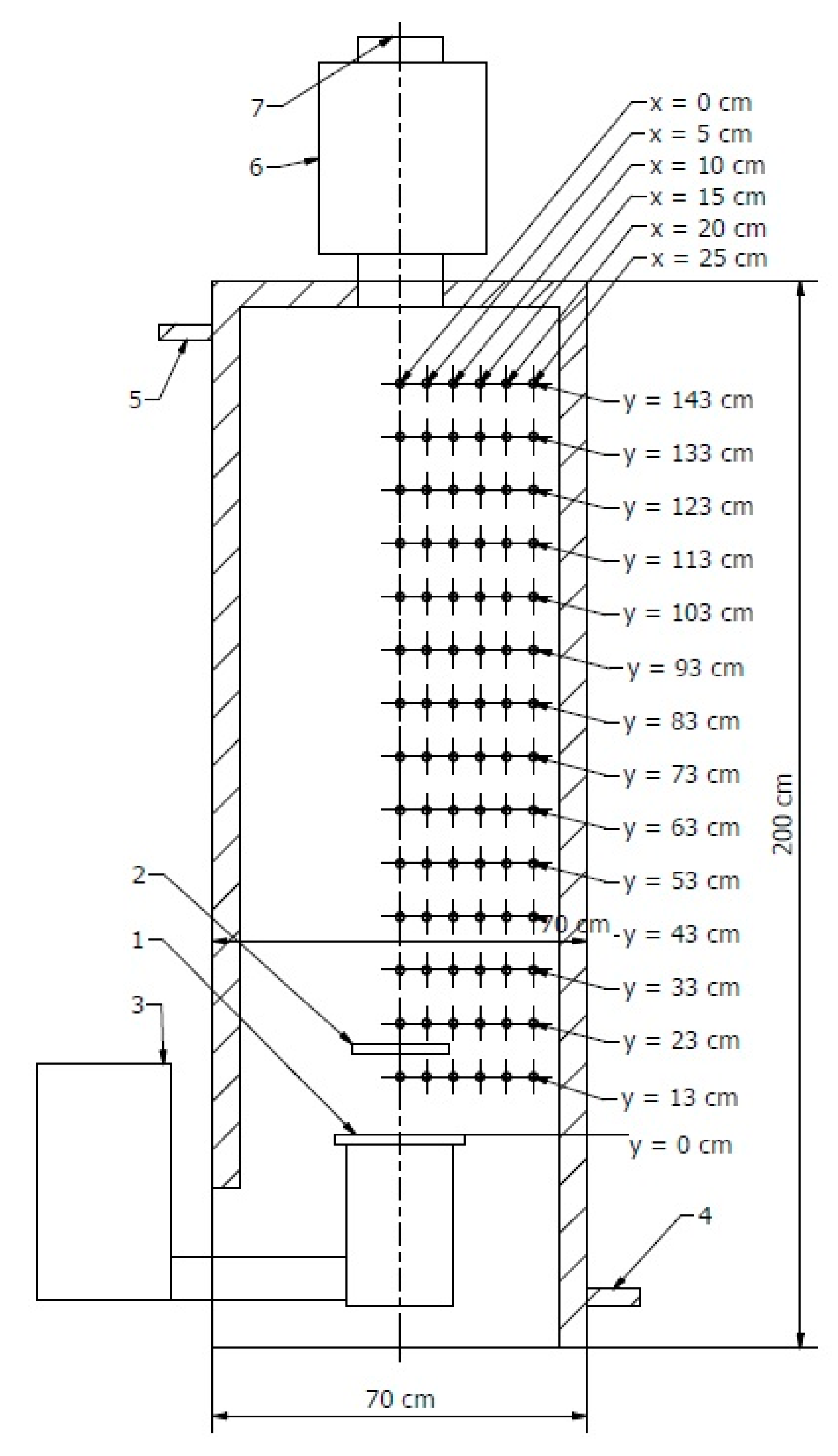
A cylindrical combustion chamber is used in the experimental part of the research. The scheme of the test stand is present in Figure 1. The heat generated from fuel combustion is transferred to the cooling water located along the cylinder side and the top surface, where a water jacket is present. A retort burner was used to form a packed bed during the research. Solid fuel with the right grain size is developed into a combustion process by a screw feeder, pushing them up. Air is supplied to the combustion process utilizing a fan. Primary air is delivered directly to the packed bed flowing through the layers of fuel.
The mentioned type of burner brings out a flame above the fuel bed. At a distance of 15 cm above the top edge of the burner, a deflector is mounted. This element is a disc-shaped cast iron element, whose main task is the dispersion of flames in the whole volume of the combustion chamber. The effect is visible in a more uniform temperature distribution inside the combustion chamber.
The test stand allows for gas temperature measurement inside the combustion chamber through 14 holes distributed every 10 cm along with chamber height according to Figure 1. The first hole was located 13 cm from the top plane of the burner (two centimeters below the bottom edge of the deflector). Measurements were done in 6 points for every plane, where the first point was present in the chamber axis. Other points were located every 5 cm in the wall direction. Because of the axisymmetric shape of the chamber, measurement was prepared only for half of the chamber. Gas temperature measurement was realized by K type thermocouples. The mentioned type of temperature detectors allows for temperature measurements down to 1200 °C.
During the experiment, exhausts gas composition was measured by the application of the Testo 350 gas analyzer. It allowed for combustion process control and was also used for quality assessment of results obtained during numerical calculations. Oxygen and carbon dioxide content in exhausts was analyzed for that purpose. Assignation of the amount of mentioned gases in exhausts allowed for validation of exhaust composition obtained during numerical analysis. A mass of particular matter present in exhausts was measured by the Testo 380 soot analyzer. The mentioned parameter was necessary for the proper determination of the exhaust gas absorption coefficient, which is crucial given the influence of a radiation heat transfer.
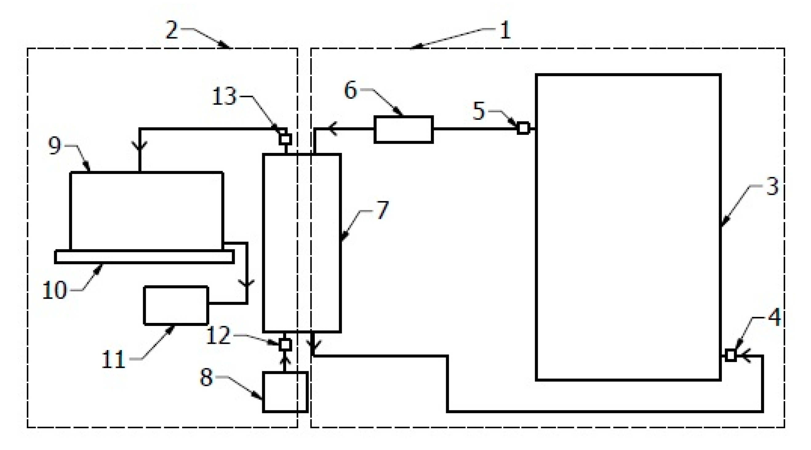
Heat received from the burning process is transported to a heat exchanger according to a scheme showed in Figure 2.
Applied installation is composed of two circuits. Water which is located in the first circuit transport heat between the test stand and the plate heat exchanger, where the mentioned heat is received by a second circuit. The temperature of cooling water was analyzed for the determination of the heating power of the test stand during the experiment. It was obtained by the application of PT100 detectors at the water inlet and outlet (points 4 and 5). Mass flow of water used for test stand cooling was measured by a heat meter equipped with a vane flow meter. The second circuit is equipped with an additional heating power check system. Water supply 8 supplied cold water to the plate heat exchanger. After heating water is directed into a bath located on a scale. The temperature of water in the second circuit is also measured by PT100 detectors (points 12 and 13). The mass flow of water flowing through the second circuit is determined based on a weight of water measured by a scale at a certain time of measurement.
2.3. Numerical Modeling
2.3.1. Domain and Mesh
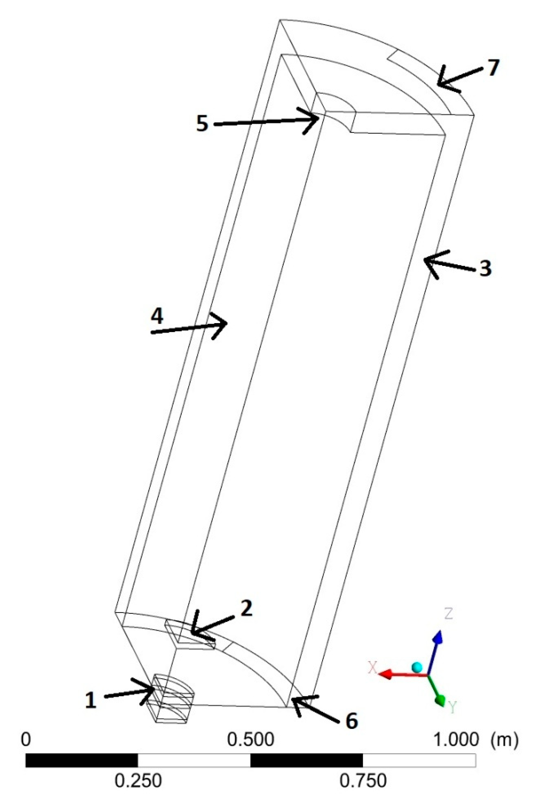
Numerical analysis of solid fuel combustion inside a fixed bed is modeled in the ANSYS Fluent software (Ansys Inc., Canonsburg, PA, USA). Numerical calculations are realized in a steady state due to high thermal inertia during heating boiler work. Results obtained during experimental research after averaging were compared with a steady-state numerical solution. Calculations were made for one-fourth part of the cylindrical combustion chamber used over the experiment due to the symmetry of the domain. The geometrical model used in numerical analysis is shown in Figure 3.
Calculations are prepared on a structural, hexagonal grid. The mentioned mesh was prepared in the Numeca IGG software. Optimal mesh parameters originate from the results of realized preliminary calculations. The crucial specification of the finally used grid is presented in Table 2. Dimensions of the numerical domain are consistent with a test stand used during the experimental part of the research. Dimensionless wall distance parameter y+ has a big impact on a heat flux calculation during heat transfer modeling between exhaust gas and cooling water. An appropriate number of elements in applied mesh results from a necessity of ensuring the mentioned parameter close to 1. Then the first layer of grid located near to heat transfer wall for both fluids taking part in conjugate heat transfer allows for the calculation of a heat flux value complied with experimental analysis.
2.3.2. Setup
A discrete phase model is used for packed bed modeling. A solid fuel fixed bed is modeled by spherical particles that are tightly packed in the bottom part of the domain according to Figure 3. The size of particles is uniform and complies with the average size of fuels used during the experimental part. The contact of discrete particles to burner walls and relative to each other is modeled by the discrete element model. The mentioned model applies a Hertz problem basing on the Young Modulus and Poisson Ratio of materials coming into mutual contact. Fuel located inside the bed is subjected to heat and mass transfer phenomena. Five successive laws are implemented for modeling of thermal transformation of the fuel (inert heating, vaporization, boiling, devolatilization, and surface combustion). Inert heating is applied while the particle temperature is less than the vaporization temperature. The mentioned process occurs also after boiling, but when the devolatilization temperature has not been reached. It is also present after the surface combustion process, where it comes to the heating of non-flammable parts of fuel. Vaporization concerns moisture content in fuel and is present when the temperature of the droplet reaches the vaporization temperature and continues until the droplet reaches the boiling point. After reaching a boiling temperature a boiling process has been started and will be continued until a moisture fraction is present in the discrete phase. Devolatization is based on a single rate model which assumes that the rate of devolatilization is the first-order dependent on the number of volatiles remaining in the particle. After the volatile component is completely evolved, a surface reaction begins which consumes the combustible fraction of the particle [32].
A pressure drop occurred during gas flow through the fixed bed is modeled as a porous zone. A momentum source term composed of viscous and inertial loss terms is added to the standard fluid flow equations set being solved during numerical calculations. Gas flow through the packed bed is modeled as laminar. Pressure drop obtained during flow through the packed bed is calculated by the Carman-Kozeny Equation (1).
Viscous and inertial resistance magnitudes are used for the definition of source term applied during porous zone modeling. Viscous resistance is defined by inverse absolute permeability 1/k which is defined according to Equation (2). Inertial resistance is defined by inertial loss coefficient C2, which is defined as in Equation (3) [32].
The numerical model of solid fuel combustion is based on fast chemistry modeling. Chemical reactions are modeled by the application of species transport equations. Reaction rates are shaped by the Eddy Dissipation Model (EDM) and are dependent on occurring turbulent fluctuations. Two steps of the volumetric reaction mechanism are implemented for volatile burning modeling. EDM assumed that chemical kinetic rates are considerably faster than rates of turbulent mixing. Then turbulent mixing is responsible for the reaction rate-limiting process [33].
A Reynolds-stress model (RSM) is responsible for the effects of turbulence modeling during calculations. Results obtained by the RSM model are much closer to the experimental validation relative to the utilization of k-ε or k-ω SST models, which are popularly used in industrial CFD applications.
Radiation heat transfer is modeled by a Discrete Ordinates (DO) model. The considered model solves a radiation heat transfer equation for a finite number of discrete solid angles, which are associated with a vector located in the global coordinate system. Calculations are being done for a three-dimensional domain where 8 octants are solved. The number of control angles that are used for discretization of each octant in the angular space is defined by Θ and Φ divisions (respectively polar and azimuthal angle measured in the global coordinate system). The numerical model takes into account 72 directions of vector due to the application of three Θ and Φ divisions [34].
The absorption coefficient for exhaust gas is calculated as a sum of the absorption coefficient obtained for a pure gas and a soot fraction included in the mixture. The absorption coefficient that occurred for a pure gas is calculated by a weighted sum of gray gases model (WSGGM) [35]. The influence of soot for a total absorption coefficient of exhausts is calculated based on Equation (4) [34],
where is a soot density, and are coefficients obtained by S.S. Sazhin [36] based on data obtained from [37,38].
2.3.3. Boundary Conditions
Applied boundary conditions correspond to circumstances obtained during the experimental part of the research. A mass flow of cooling water at the inlet to the test stand results from the required levels of heating power for two analyzed levels of a load. The temperature of cooling water at the inlet to the computational domain arises from the heat load obtained in the cooling installation. The test stand during work with the nominal power can transfer about 12 kW of heat to the cooling water.
The mass flow of fuel provided as a discrete phase is calculated during analytical calculations. Analytical calculations are prepared based on own measurements of calorific value, moisture, ash, and volatile content in used fuels. Other data could not be obtained experimentally by the author, like the chemical composition of fuel originate from the database [39] for the most similar founded type of fuel. The mass flow of air delivered to the burning process is also calculated analytically. Calculations are prepared by taking into account an air excess factor based on experimental measurement of average oxygen content in the exhaust gas for each of the analyzed cases as in Equation (5).
Analytical calculations were done with the assumption that the nominal power of the combustion process will equal 15 kW (3 kW intended for chimney loss and other wastes). Crucial parameters of boundary conditions at inlets to the computational domain are collected in Table 3. The mass flow used as boundary conditions is four times lower following real values because calculations are done for one-fourth of the real domain.
External walls of the domain are modeled as adiabatic. The mentioned simplification does not have a big impact on the correctness of the solution, because the difference between the temperature of external walls and ambient temperature is not so high. Heat transfer among working media is modeled as a coupled wall with an application of a shell conduction mechanism. Walls which separate both thermodynamic media are made from steel with a 5 mm thickness. Application of shell conduction mechanism allowed for heat conduction modeling in chamber walls not only in the normal direction but also along walls, which allows for obtaining a more accurate solution. Boundary conditions that occurred on deflector surfaces were defined also as adiabatic. The radiation emission factor for steel elements of the domain like walls and deflector is assumed as 0.7.
2.4. Physical Magnitudes Used for Heat Transfer Description
Numerical modeling results have been used for a description of the heat transfer phenomenon that occurred inside the combustion chamber. A heat flux density divided into a radiation and convection part has been used for it. Mentioned magnitudes have been used to describe of the overall amount of heat transferred to the cooling water by radiation and convection according to Equations (6) and (7).
The local value of the heat flux density has been used for calculation of the local distribution of a heat transfer coefficient. The heat transfer coefficient is known as a parameter describing the intensity of the occurred heat transfer process. The intensity of radiation and convection can be recognized separately based on radiation and convection heat transfer coefficient. The mentioned coefficients are calculated according to Equations (8) and (9).
The generic heat transfer coefficient is defined as a sum of the radiation and the convection factors. The heat transfer coefficient that occurred on the combustion chamber wall is dependent on a locally obtained difference between the wall temperature and the bulk-average temperature of exhaust gas. The bulk temperature of exhausts is achieved based on area-averaged temperature collected in subsequent horizontal cross-sections of the domain along to the Z dimension (Figure 3).
3. Results and Discussion
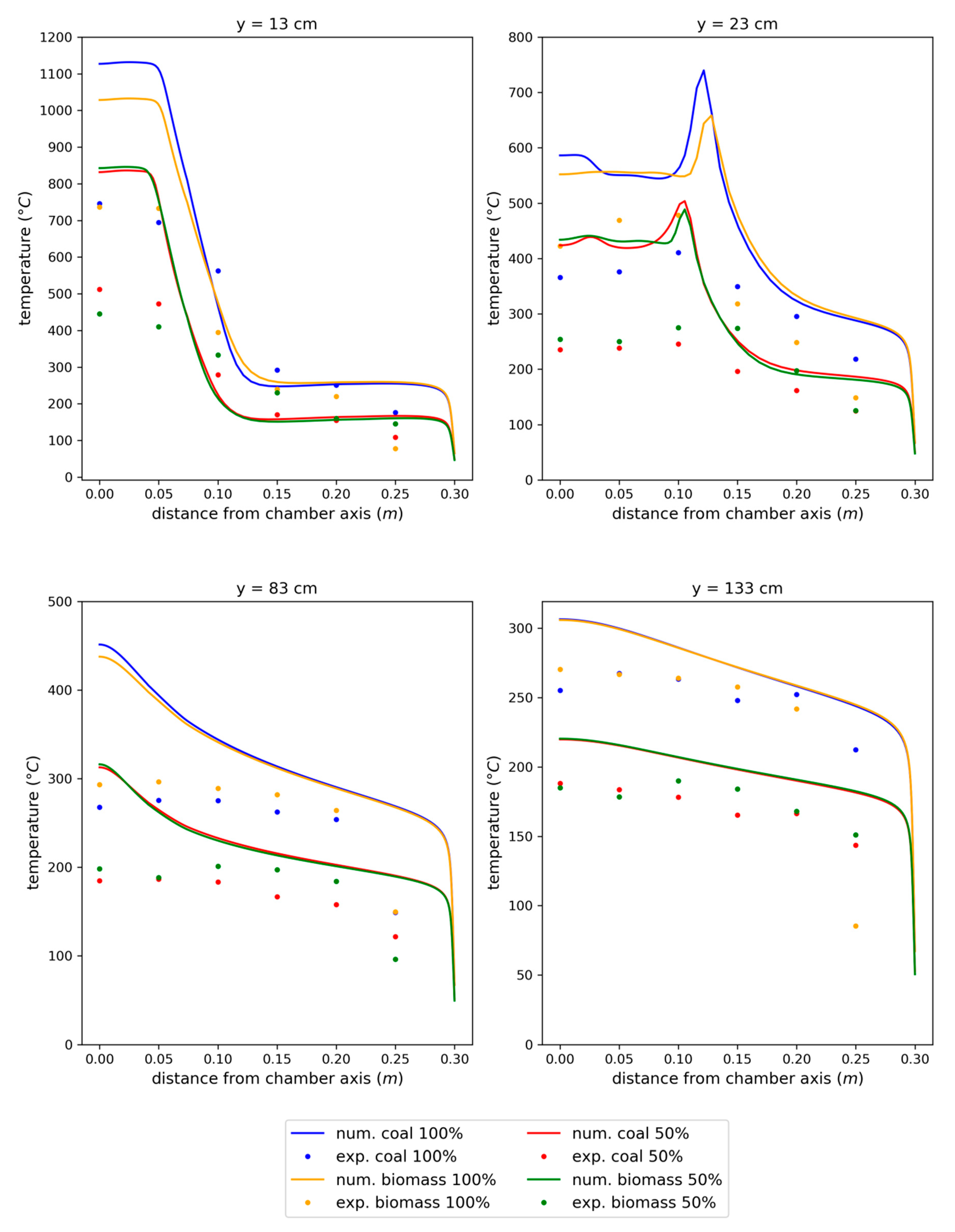
A comparison of exhaust gas temperature obtained during experimental and numerical research is shown in Figure 4. The temperature distribution is presented at four different heights of the combustion chamber representing properties obtained in three crucial parts of the chamber (two located in the burner neighborhood—bottom part, one halfway up, and one at the top of the chamber). It showed that the temperature of exhausts obtained during experimental measurements was lower relative to the numerical modeling. Especially it is well visible in the bottom part of the combustion chamber, where a temperature difference is much higher relative to higher parts of the chamber. The biggest divergence was obtained in the axis of the stand (above a burner). The highest noticed difference is equal to about 350 °C and was obtained for each of the analyzed cases. The temperature distinction decreases along the chamber radius in a wall direction. At a point located 5 cm away from the wall the temperature disparity for experimental and numerical analysis is lower and equals about 50 °C. A temperature distribution obtained during numerical modeling is getting closer to the experimental results as exhausts are moved away from the fixed bed in the vertical direction. Occurred temperature overestimation results from numerical modeling as an effect of the application of the Eddy Dissipation Model (EDM) of combustion [40,41]. EDM assumes that the realized combustion process is complete, which affects the temperature overestimation. Extermination of the mentioned phenomenon requires an application of the Eddy Dissipation Concept (EDC) model, which is an extension of EDM [42,43]. The EDC model is highly computationally expensive due to including a detailed chemical mechanism in a turbulent flow [44].
Table 4 presents a comparison obtained for a few basic parameters connected with the combustion chamber working conditions during numerical modeling and experimental research for each of the analyzed cases. It is a heat flow transferred to the cooling water, the temperature of exhaust gas at the outlet from the domain, the temperature of cooling water at the outlet from the test stand, the cooling water temperature difference between outlet and inlet of the test stand, oxygen and carbon dioxide mass fraction in exhausts leaving the domain. Due to the inability of exhaust gas mass flow at the outlet from the combustion chamber during experimental research, the mentioned magnitude was compared with a result of analytical calculations. Time-averaged data collected during experimental research for each case separately comply with the results of numerical modeling. The amount of exhaust gas obtained during numerical simulations is consistent with analytical calculations. Collected parameters show convergence between numerical modeling and experimental validation.
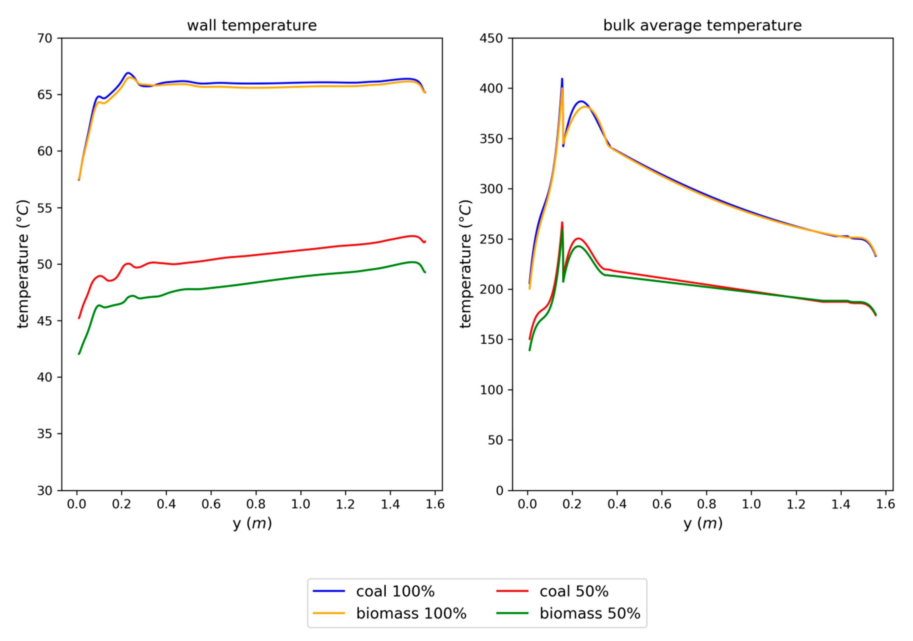
Figure 5 shows a distribution of wall temperature and a bulk-average temperature inside the chamber as a function of the domain height. The temperature of the combustion chamber wall is generally constant. It only comes to a small rising of temperature in the direction of the working medium flow (from bottom to the top of the domain), which is related to the heating of water used for test stand cooling. The average bulk temperature of exhaust gas is noticeably changing in subsequent parts of the domain.
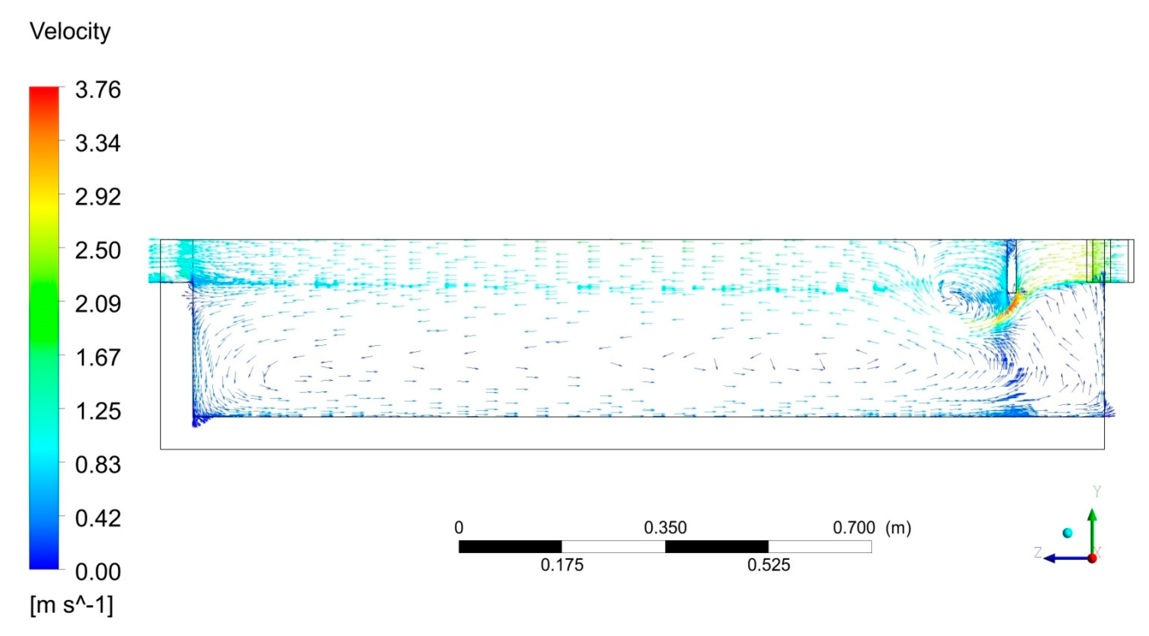
The highest value is present in a direct neighborhood of a flame. It is following the obtained data concerning overall heat flux (sum of radiation and convection heat flux), which achieves maximum value in the mentioned area. The peak of the bulk temperature occurs in the area, where a deflector limits a flame length and smashes it horizontally. When fumes flow around a deflector, the average temperature deeply decreases. Right above a deflector comes the formation of an Eddy, which causes a significant cooling of flue gas (Figure 6). Over regions of swirled flow, a visible increase of bulk temperature is present. It is caused by exhausts getting through from the flame dispersion zone to the mentioned area. In the horizontal cross-sections of the chamber located above 20 cm over a deflector, the average temperature of exhausts is gradually decreasing. Exhausts flow in the upper part of a chamber is more uniform than in the direct neighborhood of the deflector. When the gas has contact with the top surface of the combustion chamber it comes to obtain a backflow of a slight part of exhausts to the domain along heat transfer surface.
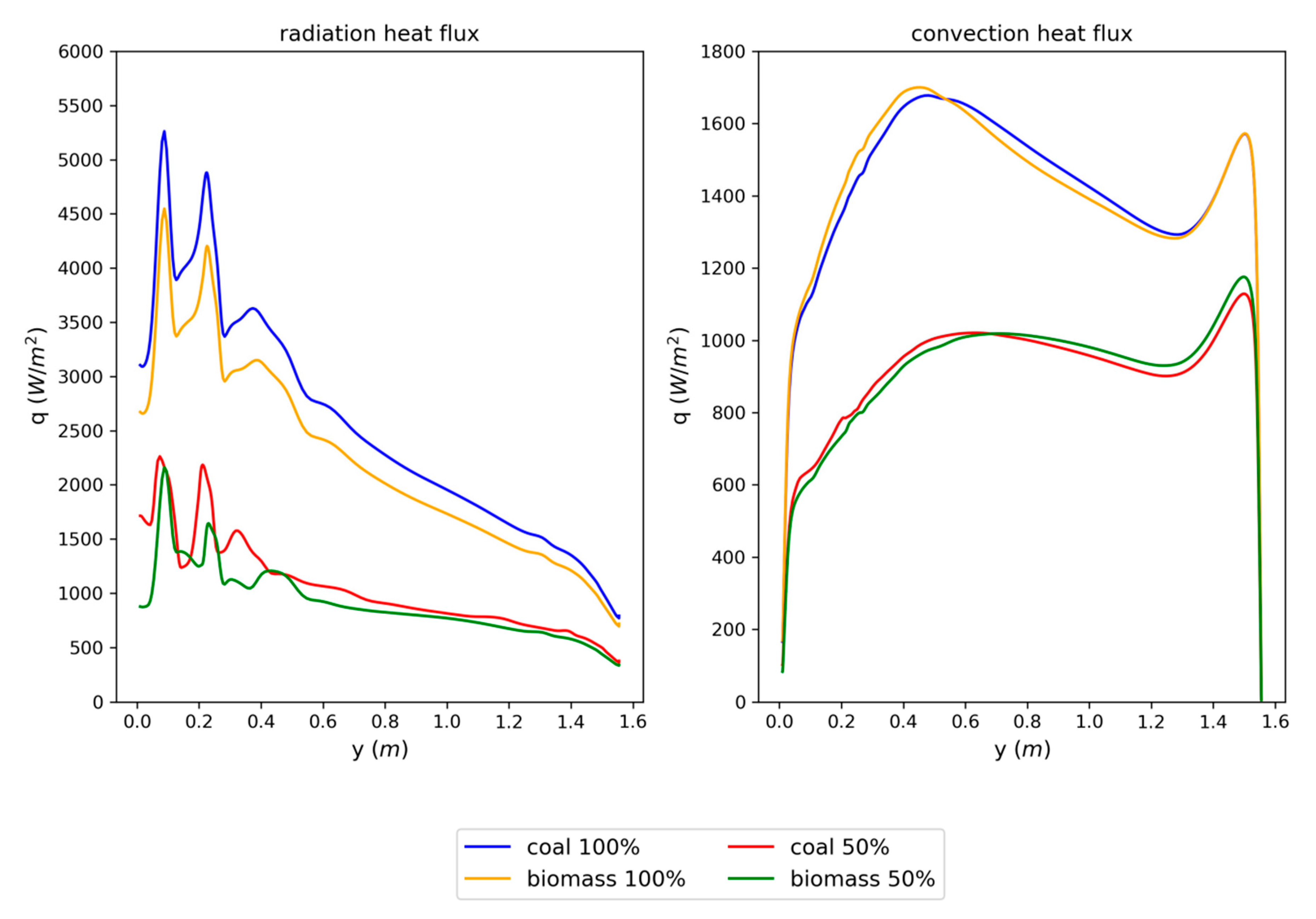
The local value of convection and radiation heat flux that occurred on the exhaust side of the combustion chamber wall along a domain height is present in Figure 7. Radiation and convection heat flux magnitudes are varied along with the height of the chamber. The impact of the radiation for an overall heat transfer process is dominating in the direct neighborhood of a flame. As a distance from a burning area is increased away, a local amount of the radiation heat flux is substantially falling off. The distribution of convective heat flux does not show significant changes over the entire surface bounding the combustion chamber. Regional increases depend on changes in the local value of the Reynolds Number and a thickness of a boundary layer. Determination of percentage participation in the heat transfer phenomenon for radiation and convection shows that they are dependent mainly on a heat load. During coal combustion with a nominal power, radiation is responsible for about 61.7% of the overall heat transfer. When combustion was carried out with the half level of the nominal heat load, radiation achieved only 50% in the heat transmission. Radiation participation in the heat transfer during biomass combustion was equal to 58.6% and 47.5%, respectively, for 100% and 50% of the nominal power.
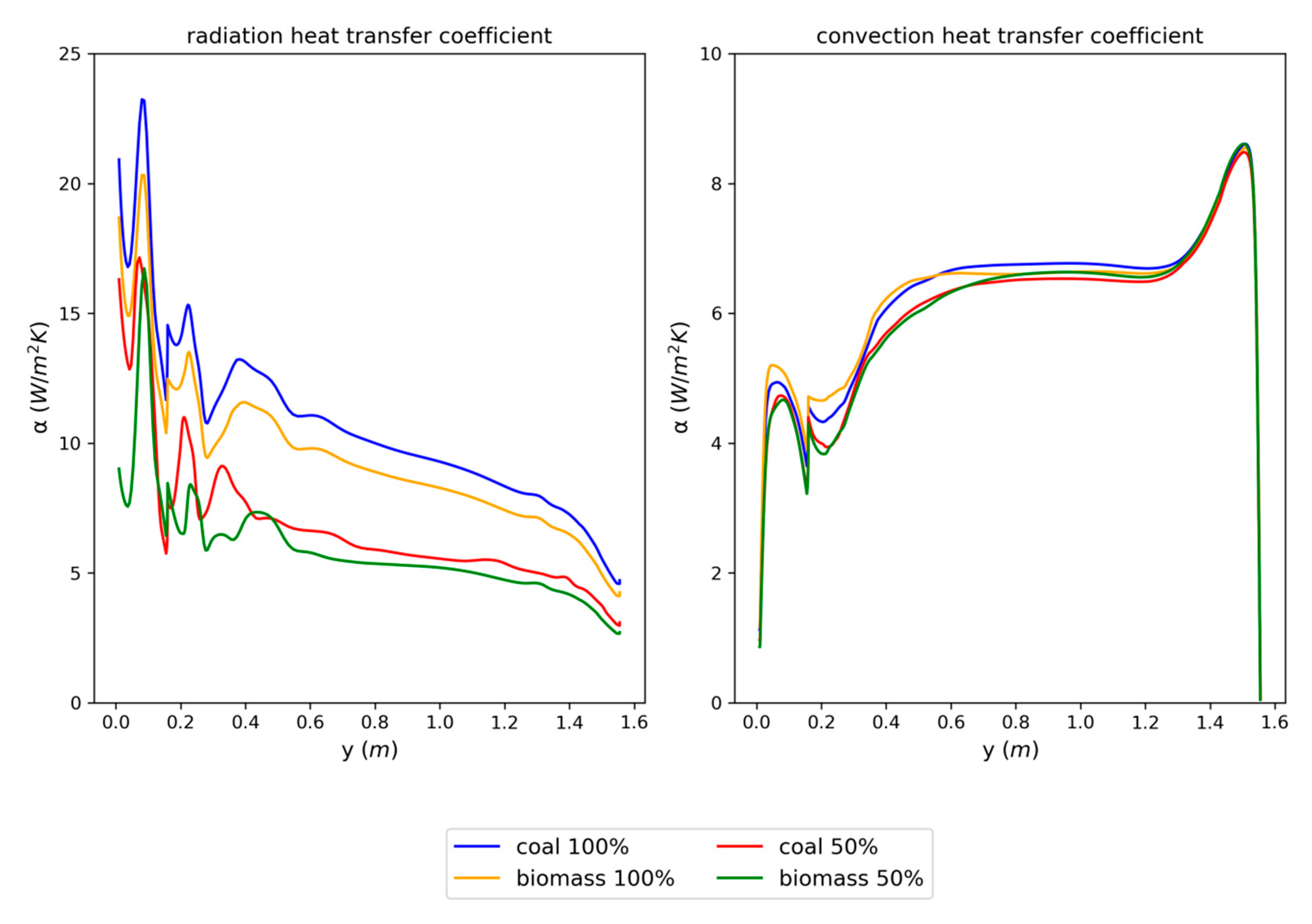
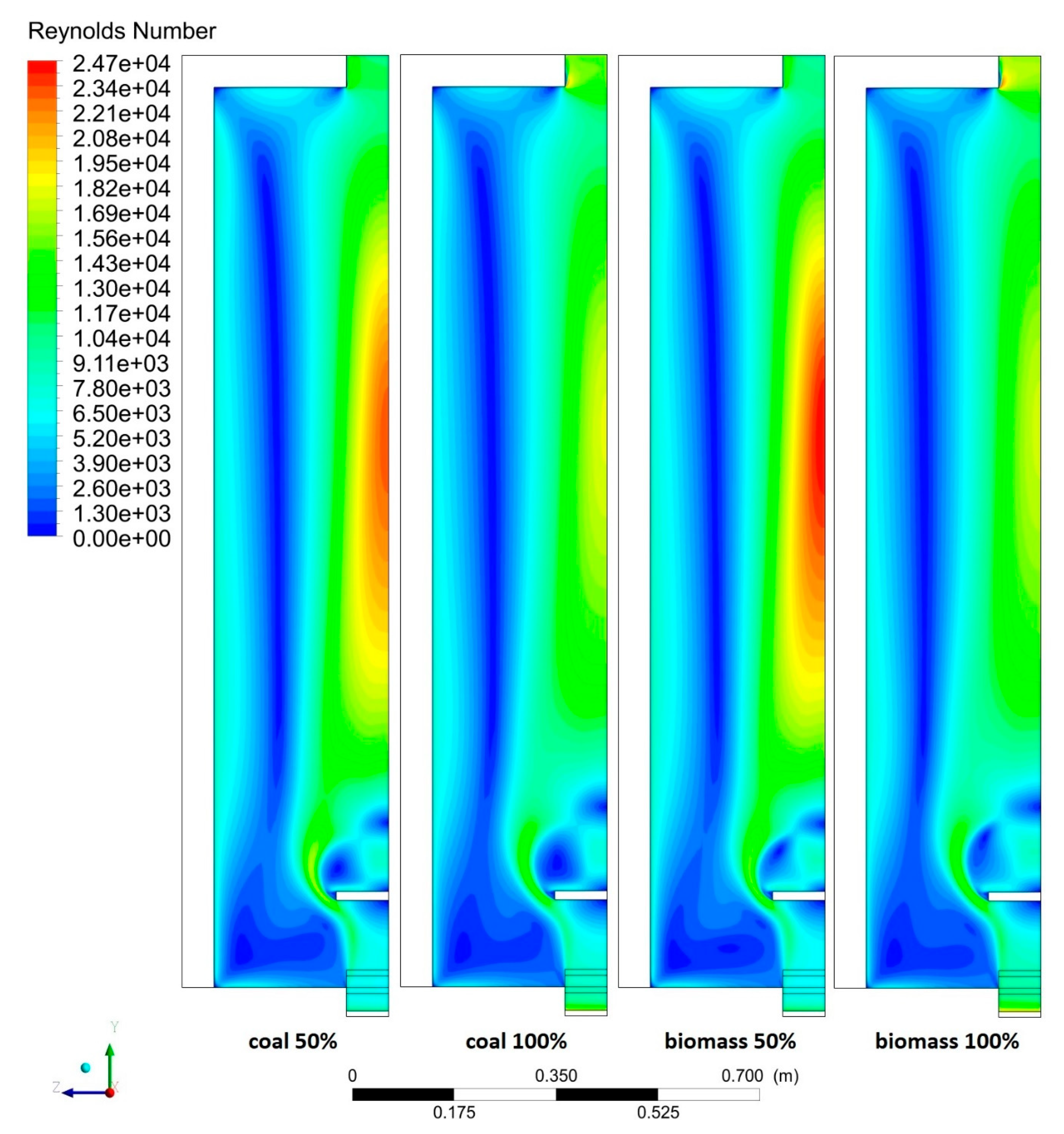
Radiation and convection heat transfer coefficient courses are various for distinct parts of the computational domain (Figure 8). The radiation heat transfer coefficient achieves a peak in the direct neighborhood of a flame and vitally decreases in the upper part of the chamber, which is following in a radiation heat flux distribution. In the bottom part of the chamber, a radiation coefficient is uneven, which testifies with a differential level of the thermal load. A varied course of the convection heat transfer coefficient has occurred along with the domain height. In the direct neighborhood of the deflector, it comes to intense decreasing of , which achieves a minimum value in the mentioned area. The convection heat transfer coefficient is increased in the area located above the deflector. After that, is stabilized until a part of the domain, which is located 15 cm below the top surface of the domain. In the last part of the domain the top surface achieves a maximum value. The peak value of the convection heat transfer coefficient is present also on the top surface of the combustion chamber. The main impact of the convection heat transfer is connected with the character of exhaust gas flow inside the combustion chamber (Figure 6). Exhaust gas movement occurred along a sidewall of the chamber and was an effect of reversing flow realized for a part of exhaust gas, which is not directly conducted to the outlet. According to theory of heat transfer [45,46], Reynolds and Prandtl numbers are the main parameters used in the analytical description of the convection heat transfer coefficient. Figure 9 shows a distribution of Reynolds number obtained during the research for analyzed cases.
A diameter of the combustion chamber is used as a characteristic linear dimension in Reynolds number definition. In the direct neighborhood of the combustion chamber sidewall, Reynolds number achieves value corresponding to a laminar or transitional flow. The effect is visible in the obtained value of which occurred during the mentioned types of fluid flow. A similar distribution of convection heat transfer coefficient between analyzed cases is connected with a lack of changes in Reynolds and Prandtl number distribution during fumes flow in the wall area.
4. Conclusions
The paper presented an experimental and numerical study on the combustion process of hard coal and biomass combustion in fixed bed conditions. Results of experimental validation and numerical modeling showed that:
- Numerical modeling of hard coal and biomass burning in fixed bed conditions allows simulating a heat transfer phenomenon that occurred in heating boilers to comply with experimental verification based on a fast chemistry model (Eddy dissipation). A numerical model to a certain extent overestimates the temperature of exhaust gas. Elimination of the mentioned overestimation requires the application of a slow chemistry model (Eddy dissipation concept), which will be developed in further research on account of high computational expense. Percentage participation of radiation and convection during the heat transfer process mostly depends on the heat load of the heating device. As the test stand works with the lower heat load, a radiation impact is decreasing.
- Heat transferred by radiation was slightly lower during biomass combustion compared with coal burning. It has to do with a smaller temperature of combustion related to a lower heating value of biomass. A higher mass flow of exhaust present in the combustion chamber has an impact on a lower temperature of burning. A greater amount of exhaust results from the higher stream of biomass required for assurance of the same level of heating power. Likewise, biomass burning has to be realized with a higher excess air coefficient, which also has a big impact on a higher amount of exhaust gas present in the combustion chamber.
- Varied fuel properties and parameters of combustion do not have a visible impact on the convection heat transfer coefficient. The main influence for the mentioned factor is connected with a local temperature difference between the wall and exhaust gas located inside a combustion chamber.
- The distribution of Reynolds number obtained near to a sidewall of the combustion chamber does not show visible differences between analyzed cases. The main impact for a Reynolds number distribution in the central part of the combustion chamber is connected with the dynamic viscosity of a flue gas, which is a function of temperature. Higher mass flow of exhausts flowing through the combustion chamber during the nominal power caused a visible decrease of Reynolds number in the central area due to exhaust gas temperature rising despite an increase of flow velocity.
- The local value of radiation and convection heat transfer coefficient are effective parameters for recognition of intensity of the heat transfer process occurring inside a heating boiler combustion chamber during packed bed combustion. Thermal devices dealing with thermodynamic processes concerning fixed bed combustion have to deal with various thermal conditions occurring in different elements responsible for the heat transfer process. The application of fast chemistry modeling for simulating conditions that occur inside the combustion chambers of solid fuel boilers is a helpful tool in the design process. A complex shape combustion chamber used during packed bed combustion can be modernized with an appropriate calculation time bearing in mind a limitation imposed during the arrangement. The effect may be visible in higher thermal efficiency of the heating boiler because of better recognition of thermal conditions that occurred during various exploitation conditions. Moreover, the results of the modeling may be applied for the preparation of certain modifications in the analytical approach of a domestic and industrial boiler design process.
Funding
The research was financed by the Poznan University of Technology financial resources for the statutory activity. The number of projects: 0712/SBAD/5166 and 0712/SBAD/5180.
Conflicts of Interest
The author declares no conflict of interest.
Nomenclature
| absorption coefficient | 1/cm | |
| A | area | m2 |
| b1 | Taylor-Foster approximation coefficient | m2/kg |
| bT | Smith approximation coefficient | 1/K |
| C2 | inertial loss coefficient | 1/m |
| CO2 | mass fraction of carbon dioxide | % |
| diameter of the volume equivalent spherical particle | m | |
| k | permeability | m2 |
| L | total height of the bed | m |
| LCV | low calorific value | MJ/kg |
| mass flow | kg/s | |
| O2 | mass fraction of oxygen | % |
| Pn | percentage level of heat load | % |
| t | temperature | °C |
| T | temperature | K |
| heat flux density | W/m2 | |
| heat flux, heating power | W | |
| superficial velocity | m/s | |
| x | horizontal distance from a cylindrical chamber axis | m |
| y | vertical distance from a burner top surface | m |
| y+ | non-dimensional wall distance | dimensionless |
| α | heat transfer coefficient | Wm−2 K−1 |
| Δp | pressure drop | Pa |
| Δt | temperature difference | °C |
| ε | bed porosity | dimensionless |
| λ | excess air coefficient | dimensionless |
| μ | dynamic viscosity | Pa·s |
| ρ | density | kg/m3 |
Abbreviations
| a | air |
| ave | average |
| con | convection |
| eg | exhaust gas |
| exp | experimental |
| f | fuel |
| in | inlet |
| mea | measured |
| num | numerical |
| out | outlet |
| rad | radiation |
| s | soot |
| w | water |
References
- Statistics Poland. Energy Consumption in Polish Households in 2018; Statistics Poland: Warszawa, Poland, 2019. (In Polish)
- Energy Regulatory Office. Thermal Energy in Numbers—2019; Energy Regulatory Office: Warszawa, Poland, 2020. (In Polish) [Google Scholar]
- Statistics Poland. Energy from Renewable Sources in 2018; Statistics Poland: Warszawa, Poland, 2019.
- Scharler, R.; Gruber, T.; Ehrenhöfer, A.; Kelz, J.; Bardar, R.M.; Bauer, T.; Hochenauer, C.; Anca-Couce, A. Transient CFD simulation of wood log combustion in stoves. Renew. Energy 2020, 145, 651–662. [Google Scholar] [CrossRef]
- Wiese, J.; Wissing, F.; Höhner, D.; Wirtz, S.; Scherer, V.; Ley, U.; Behr, H.M. DEM/CFD modeling of the fuel conversion in a pellet stove. Fuel Process. Technol. 2016, 152, 223–239. [Google Scholar] [CrossRef]
- Mehrabian, R.; Zahirovic, S.; Scharler, R.; Obernberger, I.; Kleditzsch, S.; Wirtz, S.; Scherer, V.; Lu, H.; Baxter, L.L. A CFD model for thermal conversion of thermally thick biomass particles. Fuel Process. Technol. 2012, 95, 96–108. [Google Scholar] [CrossRef]
- Gómez, M.A.; Porteiro, J.; de la Cuesta, D.; Patiño, D.; Míguez, J.L. Numerical simulation of the combustion process of a pellet-drop-feed boiler. Fuel 2016, 184, 987–999. [Google Scholar] [CrossRef]
- Gómez, M.A.; Porteiro, J.; De la Cuesta, D.; Patiño, D.; Míguez, J.L. Dynamic simulation of a biomass domestic boiler under thermally thick considerations. Energy Convers. Manag. 2017, 140, 260–272. [Google Scholar] [CrossRef]
- Gómez, M.A.; Martín, R.; Chapela, S.; Porteiro, J. Steady CFD combustion modeling for biomass boilers: An application to the study of the exhaust gas recirculation performance. Energy Convers. Manag. 2019, 179, 91–103. [Google Scholar] [CrossRef]
- Gómez, M.A.; Porteiro, J.; Patiño, D.; Míguez, J.L. Eulerian CFD modelling for biomass combustion. Transient simulation of an underfeed pellet boiler. Energy Convers. Manag. 2015, 101, 666–680. [Google Scholar] [CrossRef]
- Mehrabian, R.; Shiehnejadhesar, A.; Scharler, R.; Obernberger, I. Multi-physics modelling of packed bed biomass combustion. Fuel 2014, 122, 164–178. [Google Scholar] [CrossRef]
- Collazo, J.; Porteiro, J.; Patiño, D.; Granada, E. Numerical modeling of the combustion of densified wood under fixed-bed conditions. Fuel 2012, 93, 149–159. [Google Scholar] [CrossRef]
- Ryfa, A.; Buczynski, R.; Chabinski, M.; Szlek, A.; Bialecki, R.A. Decoupled numerical simulation of a solid fuel fired retort boiler. Appl. Therm. Eng. 2014, 73, 794–804. [Google Scholar] [CrossRef]
- Buczyński, R.; Weber, R.; Szlęk, A. Innovative design solutions for small-scale domestic boilers: Combustion improvements using a CFD-based mathematical model. J. Energy Inst. 2015, 88, 53–63. [Google Scholar] [CrossRef]
- Chaney, J.; Liu, H.; Li, J. An overview of CFD modelling of small-scale fixed-bed biomass pellet boilers with preliminary results from a simplified approach. Energy Convers. Manag. 2012, 63, 149–156. [Google Scholar] [CrossRef]
- Chapela, S.; Porteiro, J.; Míguez, J.L.; Behrendt, F. Eulerian CFD fouling model for fixed bed biomass combustion systems. Fuel 2020, 278, 118251. [Google Scholar] [CrossRef]
- Tu, Y.; Yang, W.; Siah, K.B.; Prabakaran, S. Effect of different operating conditions on the performance of a 32 MW woodchip-fired grate boiler. Energy Procedia 2019, 158, 898–903. [Google Scholar] [CrossRef]
- Tu, Y.; Zhou, A.; Xu, M.; Yang, W.; Siah, K.B.; Subbaiah, P. NOX reduction in a 40 t/h biomass fired grate boiler using internal flue gas recirculation technology. Appl. Energy 2018, 220, 962–973. [Google Scholar] [CrossRef]
- Silva, J.; Teixeira, J.; Teixeira, S.; Preziati, S.; Cassiano, J. CFD Modeling of Combustion in Biomass Furnace. Energy Procedia 2017, 120, 665–672. [Google Scholar] [CrossRef]
- Rezeau, A.; Díez, L.I.; Royo, J.; Díaz-Ramírez, M. Efficient diagnosis of grate-fired biomass boilers by a simplified CFD-based approach. Fuel Process. Technol. 2018, 171, 318–329. [Google Scholar] [CrossRef]
- Bermúdez, C.A.; Porteiro, J.; Varela, L.G.; Chapela, S.; Patiño, D. Three-dimensional CFD simulation of a large-scale grate-fired biomass furnace. Fuel Process. Technol. 2020, 198, 106219. [Google Scholar] [CrossRef]
- Klason, T.; Bai, X.S.; Bahador, M.; Nilsson, T.K.; Sundén, B. Investigation of radiative heat transfer in fixed bed biomass furnaces. Fuel 2008, 87, 2141–2153. [Google Scholar] [CrossRef]
- Joachimiak, M.; Joachimiak, D.; Ciałkowski, M.; Małdziński, L.; Okoniewicz, P.; Ostrowska, K. Analysis of the heat transfer for processes of the cylinder heating in the heat-treating furnace on the basis of solving the inverse problem. Int. J. Therm. Sci. 2019, 145, 105985. [Google Scholar] [CrossRef]
- Rezazadeh, N.; Hosseinzadeh, H.; Wu, B. Effect of burners configuration on performance of heat treatment furnaces. Int. J. Heat Mass Transf. 2019, 136, 799–807. [Google Scholar] [CrossRef]
- Yıldız, E.; Başol, A.M.; Mengüç, M.P. Segregated modeling of continuous heat treatment furnaces. J. Quant. Spectrosc. Radiat. Transf. 2020, 249, 106993. [Google Scholar] [CrossRef]
- Gautam, A.; Saini, R.P. Experimental investigation of heat transfer and fluid flow behavior of packed bed solar thermal energy storage system having spheres as packing element with pores. Sol. Energy 2020, 204, 530–541. [Google Scholar] [CrossRef]
- Barde, A.; Nithyanandam, K.; Shinn, M.; Wirz, R.E. Sulfur heat transfer behavior for uniform and non-uniform thermal charging of horizontally-oriented isochoric thermal energy storage systems. Int. J. Heat Mass Transf. 2020, 153, 119556. [Google Scholar] [CrossRef]
- Ziegler, B.; Mosiężny, J.; Czyżewski, P. Unsteady CHT analysis of a solid state, sensible heat storage for PHES system. Int. J. Numer. Methods Heat Fluid Flow 2019. [Google Scholar] [CrossRef]
- Taler, D.; Taler, J.; Trojan, M. Thermal calculations of plate–fin–and-tube heat exchangers with different heat transfer coefficients on each tube row. Energy 2020, 203, 117806. [Google Scholar] [CrossRef]
- Li, N.; Chen, J.; Cheng, T.; Klemeš, J.J.; Varbanov, P.S.; Wang, Q.; Yang, W.; Liu, X.; Zeng, M. Analysing thermal-hydraulic performance and energy efficiency of shell-and-tube heat exchangers with longitudinal flow based on experiment and numerical simulation. Energy 2020, 202, 117757. [Google Scholar] [CrossRef]
- Judt, W.; Bartoszewicz, J. Analysis of fluid flow and heat transfer phenomenon in a modular heat exchanger. Heat Transf. Eng. 2019, in press. [Google Scholar] [CrossRef]
- ANSYS Inc. ANSYS FLUENT User Guide; 18.2.; ANSYS Inc.: Canonsburg, PA, USA, 2017. [Google Scholar]
- Vasquez, E.R.; Eldredge, T. Process modeling for hydrocarbon fuel conversion. In Advances in Clean Hydrocarbon Fuel Processing: Science and Technology; Elsevier Ltd.: Amsterdam, The Netherlands, 2011; pp. 509–545. ISBN 9781845697273. [Google Scholar]
- ANSYS Inc. ANSYS Fluent Theory Guide; 18.2; ANSYS Inc.: Canonsburg, PA, USA, 2017. [Google Scholar]
- Tae-Ho, S. Comparison of engineering models of nongray behavior of combustion products. Int. J. Heat Mass Transf. 1993, 36, 3975–3982. [Google Scholar] [CrossRef]
- Sazhin, S.S. An Approximation for the Absorption Coefficient of Soot in a Radiating Gas; Manuscript, Fluent Europe, Ltd.: Sheffield, UK, 1994. [Google Scholar]
- Smith, T.F.; Shen, Z.F.; Friedman, J.N. Evaluation of coefficients for the weighted sum of gray gases model. J. Heat Transf. 1982, 104, 602–608. [Google Scholar] [CrossRef]
- Taylor, P.B.; Foster, P.J. The total emissivities of luminous and non-luminous flames. Int. J. Heat Mass Transf. 1974, 17, 1591–1605. [Google Scholar] [CrossRef]
- TNO Phyllis 2. Available online: https://phyllis.nl/ (accessed on 8 September 2020).
- Zubanov, V.M.; Stepanov, D.V.; Shabliy, L.S. The technique for Simulation of Transient Combustion Processes in the Rocket Engine Operating with Gaseous Fuel “hydrogen and Oxygen”. J. Phys. Conf. Ser. 2017, 803, 012187. [Google Scholar] [CrossRef] [Green Version]
- Yadav, S.; Mondal, S.S. Modelling of oxy-pulverized coal combustion to access the influence of steam addition on combustion characteristics. Fuel 2020, 271, 117611. [Google Scholar] [CrossRef]
- Jójka, J.; Ślefarski, R. Dimensionally reduced modeling of nitric oxide formation for premixed methane-air flames with ammonia content. Fuel 2018, 217, 98–105. [Google Scholar] [CrossRef]
- Lewandowski, M.T.; Parente, A.; Pozorski, J. Generalised Eddy Dissipation Concept for MILD combustion regime at low local Reynolds and Damköhler numbers. Part 1: Model framework development. Fuel 2020, 278. [Google Scholar] [CrossRef]
- Bösenhofer, M.; Wartha, E.M.; Jordan, C.; Harasek, M. The eddy dissipation concept-analysis of different fine structure treatments for classical combustion. Energies 2018, 11, 1902. [Google Scholar] [CrossRef] [Green Version]
- Rohsenow, W.; Hartnett, J. Handbook of Heat Transfer; McGraw-Hill Education: New York, NY, USA, 1999; ISBN 0070535558. [Google Scholar]
- Serth, R.W. Process Heat Transfer: Principles and Applications; Elsevier Academic Press: Cambridge MA, USA, 2007; ISBN 9780080544410. [Google Scholar]
Figure 1.
Scheme of a cylindrical chamber with marked measurement points used during the experiment, 1—retort feeder, 2—deflector, 3—fuel tray, 4—water inlet, 5—water outlet, 6—insulated measurement duct, 7—flue gas outlet to the chimney.
Figure 1.
Scheme of a cylindrical chamber with marked measurement points used during the experiment, 1—retort feeder, 2—deflector, 3—fuel tray, 4—water inlet, 5—water outlet, 6—insulated measurement duct, 7—flue gas outlet to the chimney.

Figure 2.
Scheme of a cooling system, 1—first circuit of water flow, 2—second circuit of water flow, 3—combustion chamber, 4—PT100 measurement point at inlet to test stand, 5—PT100 measurement point at outlet from test stand, 6—vane flow meter, 7—plate heat exchanger, 8—cold water supply, 9—bath, 10—scale, 11—hot water drain, 12—PT100 measurement point at inlet to the heat exchanger for water in secondary circuit, 13—PT100 measurement point at outlet from the heat exchanger for water in secondary circuit.

Figure 3.
Overview on a computational domain, 1—volume of fixed bed, 2—deflector, 3—water jacket, 4—combustion chamber, 5—exhaust gas outlet, 6—cooling water inlet, 7—cooling water outlet.
Figure 3.
Overview on a computational domain, 1—volume of fixed bed, 2—deflector, 3—water jacket, 4—combustion chamber, 5—exhaust gas outlet, 6—cooling water inlet, 7—cooling water outlet.

Figure 4.
Comparison of an exhaust gas temperature distribution at different heights in the combustion chamber obtained from an experimental and a numerical part of the research.
Figure 4.
Comparison of an exhaust gas temperature distribution at different heights in the combustion chamber obtained from an experimental and a numerical part of the research.

Figure 5.
Distribution of exhaust gas temperature located in a layer neighboring with the combustion chamber wall and a bulk area-average temperature of flue gas as a function of chamber height.
Figure 5.
Distribution of exhaust gas temperature located in a layer neighboring with the combustion chamber wall and a bulk area-average temperature of flue gas as a function of chamber height.

Figure 6.
Visualization of the character of a flow inside a combustion chamber.

Figure 7.
Distribution of radiation and convection heat flux obtained on the flue gas side of a chamber wall as a function of combustion chamber height.
Figure 7.
Distribution of radiation and convection heat flux obtained on the flue gas side of a chamber wall as a function of combustion chamber height.

Figure 8.
Distribution of radiation and convection heat transfer coefficient obtained on the flue gas side of a chamber wall as a function of combustion chamber height.
Figure 8.
Distribution of radiation and convection heat transfer coefficient obtained on the flue gas side of a chamber wall as a function of combustion chamber height.

Figure 9.
Reynolds number distribution obtained for each of the analyzed cases.


Table 1.
Proximate and ultimate analysis of used fuels.
| Parameter | Hard Coal | Biomass |
|---|---|---|
| moisture (%) | 5.8 | 5 |
| ash (%) | 3.4 | 0.4 |
| volatile (%) | 31.5 | 77 |
| carbon (%) | 75.6 | 46.6 |
| hydrogen (%) | 4.2 | 5.5 |
| oxygen (%) | 9.3 | 40.9 |
| nitrogen (%) | 1.4 | 1.2 |
| sulphur (%) | 0.4 | 0.4 |
| LCV (MJ/kg) | 29 | 18 |
Table 2.
Parameters of the grid used in numerical calculations.
| Parameter | Value |
|---|---|
| number of cells | 2.9 M |
| y+ | ≈1 |
| minimum orthogonal quality | 0.82 |
| maximum skewness | 0.39 |
Table 3.
Crucial physical magnitudes used as boundary conditions in the inlet to the numerical domain.
Table 3.
Crucial physical magnitudes used as boundary conditions in the inlet to the numerical domain.
| Fuel | Hard Coal | Biomass | ||
|---|---|---|---|---|
| (%) | 50% | 100% | 50% | 100% |
| (kg/s) | 50% | 100% | 50% | 100% |
| (kg/s) | 5.7 × 10⁻² | 9.2 × 10⁻² | 5.7 × 10⁻² | 9.2 × 10⁻² |
| (kg/s) | 7.1 × 10⁻⁵ | 1.4 × 10⁻⁴ | 1.1 × 10⁻⁴ | 2.2 × 10⁻⁴ |
| (°C) | 7.7 × 10⁻³ | 1.0 × 10⁻² | 7.0 × 10⁻³ | 1.1 × 10⁻² |
Table 4.
Comparison of crucial parameters obtained in numerical and experimental (analytical) part of the research.
Table 4.
Comparison of crucial parameters obtained in numerical and experimental (analytical) part of the research.
| Case | Experimental/Analytical Data | Numerical Data | ||||||
|---|---|---|---|---|---|---|---|---|
| Fuel | Hard Coal | Biomass | Hard Coal | Biomass | ||||
| (%) | 50% | 100% | 50% | 100% | 50% | 100% | 50% | 100% |
| (kW) | 6.5 | 11.7 | 6.2 | 11.7 | 6.5 | 12.6 | 6.2 | 11.7 |
| (°C) | 177.8 | 276.3 | 180.4 | 266.5 | 189.8 | 258.5 | 190.6 | 259.7 |
| (kg/s) | 0.80 × 10⁻² | 1.09 ×10⁻² | 0.75 × 10⁻² | 1.17 × 10⁻² | 0.80 × 10⁻² | 1.11 × 10⁻² | 0.75 × 10⁻² | 1.18 × 10⁻² |
| (°C) | 49.2 | 60.6 | 46.7 | 61.2 | 48.9 | 61.2 | 46.5 | 61.1 |
| (°C) | 6.9 | 7.7 | 6.6 | 7.7 | 6.6 | 8.2 | 6.3 | 7.6 |
| O2, out (%) | 14.2 | 10.0 | 13.8 | 11.2 | 13.9 | 9.6 | 14.1 | 11.6 |
| CO2, out (%) | 7.0 | 10.1 | 7.0 | 9.1 | 7.4 | 10.8 | 9.8 | 12.5 |
Publisher’s Note: MDPI stays neutral with regard to jurisdictional claims in published maps and institutional affiliations. |
© 2020 by the author. Licensee MDPI, Basel, Switzerland. This article is an open access article distributed under the terms and conditions of the Creative Commons Attribution (CC BY) license (http://creativecommons.org/licenses/by/4.0/).
Share and Cite
MDPI and ACS Style
Judt, W. Numerical and Experimental Analysis of Heat Transfer for Solid Fuels Combustion in Fixed Bed Conditions. Energies 2020, 13, 6141. https://doi.org/10.3390/en13226141
AMA Style
Judt W. Numerical and Experimental Analysis of Heat Transfer for Solid Fuels Combustion in Fixed Bed Conditions. Energies. 2020; 13(22):6141. https://doi.org/10.3390/en13226141
Chicago/Turabian StyleJudt, Wojciech. 2020. "Numerical and Experimental Analysis of Heat Transfer for Solid Fuels Combustion in Fixed Bed Conditions" Energies 13, no. 22: 6141. https://doi.org/10.3390/en13226141
Note that from the first issue of 2016, this journal uses article numbers instead of page numbers. See further details here.