Hybrid Energy Systems Sizing for the Colombian Context: A Genetic Algorithm and Particle Swarm Optimization Approach

Abstract

The use of fossil resources for electricity production is one of the primary reasons for increasing greenhouse emissions and is a non-renewable resource. Therefore, the electricity generation by wind and solar resources have had greater applicability in recent years. Hybrid Renewable Energy Systems (HRES) integrates renewable sources and storage systems, increasing the reliability of generators. For the sizing of HRES, Artificial Intelligence (AI) methods such as Genetic Algorithms (GA) and Particle Swarm Optimization (PSO) stand out. This article presents the sizing of an HRES for the Colombian context, taking into account the energy consumption by three typical demands, four types of wind turbines, three types of solar panels, and a storage system for the system configuration. Two optimization approaches were set-up with both optimization strategies (i.e., GA and PSO). The first one implies the minimization of the Loss Power Supply Probability (LPSP). In contrast, the second one concerns adding the Total Annual Cost (TAC) or the Levelized Cost of Energy (LCOE) to the objective function. Results obtained show that HRES can supply the energy demand, where the PSO method gives configurations that are more adjusted to the considered electricity demands.

1. Introduction

Electricity is a commodity highly demanded around the world, generated from primary forms of energy such as fossil fuels (e.g., natural gas, coal, among others) and renewable sources (i.e., biomass, hydro, wind, solar, etc.) [1]. About 80% of worldwide energy demand is supplied from fossil resources [2], and only 20% with renewable sources [3]; such exploitation of fossil resources showed an annual average increase of 1.3% in $\mathrm{C}{\mathrm{O}}_2$ emissions in the last five years [4]. In this sense, the need arises to use clean technologies which do not harm the environment. Regarding the Colombian context, the electricity sector in 2014 represented 17% of the final energy consumed; 67% came from hydroelectric plants with an installed capacity greater than 20 MW, 2.5% to hydroelectric plants between 10 MW and 20 MW, and 1.3% to small hydroelectric plants with capacities less than 10 MW. On the other side, 28.5% of electricity was produced with fossil fuels in thermal plants, representing an installed capacity greater than 20 MW, 0.6% to fossil thermal and co-generation plants with less than 20 MW; 0.5% to biomass co-generation plants and, only 0.1%, to wind generation [3].

In 2016, the electric power coverage indices through the Colombian territory showed a deficit in the energy supply. The Vichada and Vaupés regions presented around 60% of energy coverage, followed by the Amazonas and Guaviare regions with about 75%. For its part, La Guajira, despite its wealth of natural resources for power generation, stood out with coverage of the electricity supply less than 80% [5]. 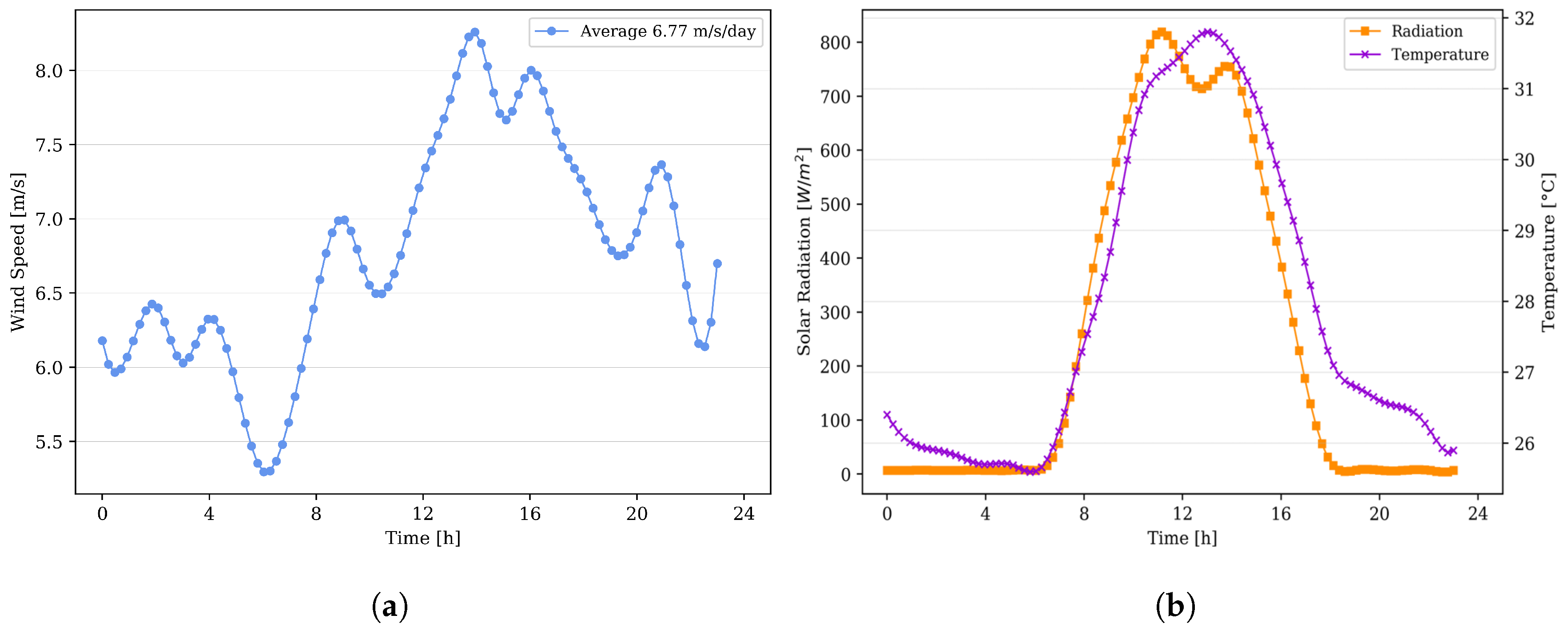Additionally, in the year 2017, approximately 52% of the Colombian territory was characterized by being non-interconnected areas, defined as regions with high costs of providing electric power service, high levels of loss in electrical generation, and unsatisfied basic needs above 77% [6]. The characteristics of the natural resources and the coverage index in Colombia allow for inferring that the implementation of energy systems that take advantage of natural resources can increase the country’s energy supply coverage. The wind resource in La Guajira is considered one of the best in South America, with a probability of around 82% of having multi-annual wind speeds between 4 m/s and 9 m/s [7], meaning a possible installed capacity of 18 GW [3]. On the other hand, from the solar resource point of view, Colombia has average irradiation of 4.5 kW-h/m${}^2$/day, higher than the global average 3.9 kW-h/m${}^2$/day. In some regions, average values up to 6 kW-h/m${}^2$/day are reached, such as La Guajira, the Atlantic Coast, Arauca, Casanare, Vichada, and Meta [3].

Regarding the energy prices in Colombian, it can be classified by regions that have a connection to the national transmission system and non-interconnected areas. In 2019, the areas covered by the transmission system presented prices between 0.06 USD/kW-h and 0.19 USD/kW-h, depending on the residential sector [8]. On the other hand, in 2017, energy prices for non-interconnected areas ranged between 0.18 USD/kW-h and 0.48 USD/kWh, corresponding to Isla Fuerte in Córdoba and the municipality of Caruru in Vaupés [6]. Moreover, some non-interconnected regions had conventional energy systems like diesel generators to provide electrical energy partially. The energy supply prices reached values of 0.28 USD/kW-h; it took into account fuel cost and operation and maintenance expenditures [9]. The related costs to the wind and solar generation have been reduced in the last decade [10], allowing them to compete with the prices of traditional plants running on fossil fuels [1]. Until 2017, the Levelized Cost of Energy through wind energy and photo-voltaic systems reached mean values of 0.05 USD/kW-h and 0.1 USD/kW-h, respectively [11]. In comparison with the related prices for the Colombian territory, it is possible to conclude that the cost of energy supply derived from natural resources can take values within the range of prices characteristic of a non-interconnected area and regions covered by the national transmission system.

The main disadvantage of wind and solar sources is its variability in time due to both resources’ intermittent nature. However, a hybrid system can integrate these two energy sources with a storage system such as a storage system [12], Pump Storage Hydroelectric system (PSH) [13] or other energy storage systems [14], aiming for the possibility to supply the energy demand of a particular region [15,16]. HRES mathematical models are usually not easy to describe, either by the number of variables, their complex interaction, or the relationships implicit in its formulation [17]. For this reason, some authors employed heuristic optimization techniques for searching for the best solution or the variables’ values that fulfill an objective function [18], such as Genetic Algorithms (GA) and Particle Swarm Optimization (PSO) [19]. Particle Swarm Optimization (PSO) and Genetic Algorithms (GA) share computational methods based on Evolutionary Algorithms (EA). PSO is inspired by the behavior of flocks of birds and fishes [17], while GA combines exhaustive search techniques and the natural principles of evolution [20].

Some authors have carried out the sizing of HRES by GA and PSO. Khatib et al. [21] combined iterative search and GA, and Kamjoo et al. [22] employed the Non-dominant Sorting Genetic Algorithm (NSGA), both for the sizing of a microgrid with photo-voltaic panels, wind turbines, and storage system. Merei et al. [23] used a GA considering three different battery technologies. In contrast, Borhanazad et al. [24] used a multi-objective PSO, modeling the cost of energy (COE) and LPSP, for the sizing of an HRES composed of photo-voltaic panels, wind turbines, diesel plant, and storage system. Recently, Barrozo-Budes et al. [25] developed a technical-economic analysis of a hybrid system consisting of wind and solar energy, using HOMER Pro software for the region of Puerto Bolívar, La Guajira, in Colombia. Khare et al. [19] studied the systems consisting of solar and wind technologies and focuses on the review of evolutionary techniques for optimization, where GA and PSO stand out. A well-suited HRES, in terms of size and location, can improve life quality, especially to people in regions where the electricity supply is not covered. As energy coverage expands, energy equity and environmental sustainability are promoted, allowing them to attend the World Energy Council (WEC) energy rating requirements [26].

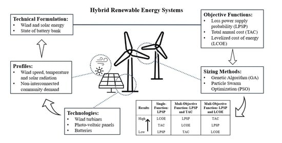
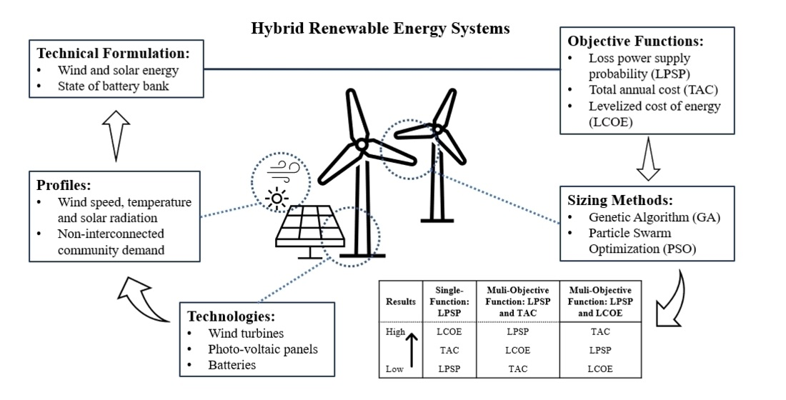
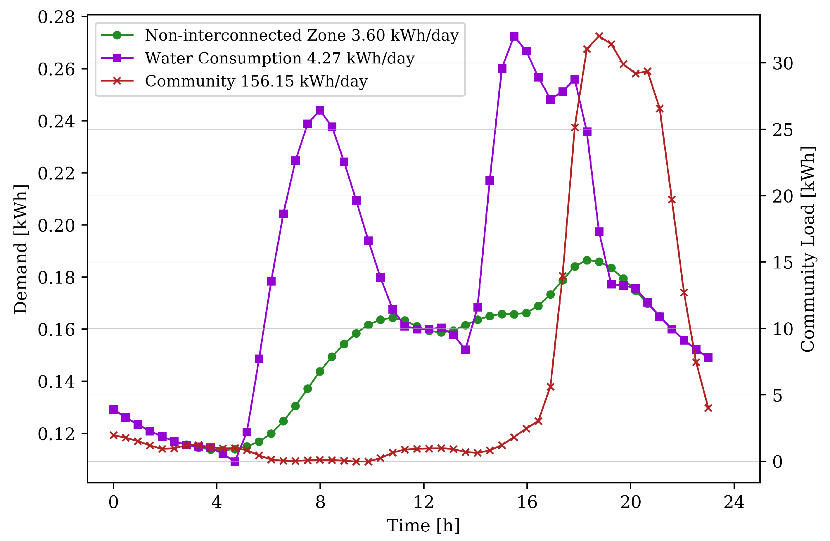
Considering the Colombian context, in terms of energy costs (mainly dominated by hydro-power plants) and the lack of electricity reliability in some regions, this work studies conditions that constrain and potentiate the sizing and implementation of HRES, including wind and solar resources availability and electricity demand. By this, optimization methods such as GA and PSO and objective functions, including LPSP, TAC, and LCOE, are used for sizing HRES systems. Additionally, a sensitivity analysis concerning a demand is proposed, considering the energy expenditure of a single residence with and without drinking water consumption and the energy demand of a representative population of a non-interconnected zone in Colombia. Section 2 presents the formulation of the technologies considered, the estimation of the study demands, and the objective functions. Section 3 describes the technical specifications of the equipment treated, the demand profiles, wind speed, solar radiation and temperature, and, finally, the GA and PSO methods are presented. Section 4 and Section 5 present and discuss the results, and Section 6 concludes the study.

2. Formulation

This section presents the mathematical models related to wind energy, solar energy, battery status under charge, and discharge restrictions, and the energy generated by the HRES. Additionally, the objective functions for sizing and modeling energy expenditure for drinking water consumption in a typical Colombian non-interconnected zone are presented.

2.1. Wind Energy Model

Wind power generation can be evaluated as:

$$P_{wt}\left(v\right)=\frac{1}{2}{C}_p\rho A{v}^3,$$

(1)

where $P_{wt}$ denotes the power generated by the wind turbine as a function of wind speed v, $C_p$ is the wind turbine characteristic power coefficient, $\rho$ is the air density, and A is the swept area of the wind turbine rotor [27].

Each wind turbine is characterized by its speed–power curve which allows for identifying the generation start speed or “Cut-In Speed” ($V_{ci}$), the nominal speed ($V_r$), and the “Cut-Off Speed” ($V_{co}$) at which the system protects the components and does not more power is generated. The power characteristic curve given as a function of the characteristic speeds is governed by:

$$P_{wt}\left(t\right)=\left\{\begin{array}{cc}0,& \mathrm{if}v\left(t\right)<V_{ci}\\ \frac{P_r}{\left(V_r^3-V_{ci}^3\right)}{v}^3\left(t\right)-\frac{V_{ci}^3}{\left(V_r^3-V_{ci}^3\right)}{P}_r,& \mathrm{if}{V}_{ci}\le v\left(t\right)<V_r\\ P_r,& \mathrm{if}{V}_r\le v\left(t\right)<V_{co}\\ 0,& \mathrm{if}\ge V_{co}\end{array}\right.,$$

(2)

where $P_r$ is the nominal power of the wind turbine and $v\left(t\right)$ is the wind speed in an instant of time t [20].

2.2. Photo-Voltaic Energy Model

The power generation of a photo-voltaic solar system is given by:

$$P_{pv}\left(t\right)=P_{pvr}\frac{R\left(t\right)}{R_{ref}}\left(1+N_T\left(T_c\left(t\right)-T_{ref}\right)\right),$$

(3)

being

$$T_c\left(t\right)=T_{air}+\left(\frac{NOCT-20}{800}\right)R\left(t\right),$$

(4)

where $P_{pvr}$ is the nominal power of the photo-voltaic solar panel, $R\left(t\right)$ is the solar radiation in an instant of time t given in W/m${}^2$, $R_{ref}$ is the reference solar radiation of 1000 W/m${}^2$, $T_{ref}$ is the reference temperature of the solar cell (usually given as 25 °C), $N_T$ is the temperature coefficient of the photo-voltaic panel, $T_{air}$ is the ambient temperature given by temperature profile, and $NOCT$ is the operating temperature of the solar cell given in °C [28].

2.3. State of Battery Model

The state of the storage system depends on the monitoring of the demand and the renewable energy generation. If $E_{pv}\left(t\right)+E_{wt}\left(t\right)>E_{ca}\left(t\right)$, there is a charge of energy given by:

$$E_b\left(t\right)=E_b(t-1)(1-\sigma )+\left\{\frac{\left[\left(E_{pv}\left(t\right){\eta }_{inv}+E_{wt}\left(t\right){\eta }_{inv}^2\right)-\frac{E_{ca}\left(t\right)}{{\eta }_{inv}}\right]}{{\eta }_{bat}^{-1}}\right\},$$

(5)

otherwise, if $E_{pv}\left(t\right)+E_{wt}\left(t\right)<E_{ca}\left(t\right)$, there is a discharge of energy given by:

$$E_b\left(t\right)=E_b(t-1)(1-\sigma )-\left\{\frac{\left[\frac{E_{ca}\left(t\right)}{{\eta }_{inv}}-\left(E_{pv}\left(t\right){\eta }_{inv}+E_{wt}\left(t\right){\eta }_{inv}^2\right)\right]}{{\eta }_{bat}}\right\},$$

(6)

where $E_b(t-1)$ is the state of the battery at the previous moment, $\sigma$ is the hourly self-discharge ratio of the battery, ${\eta }_{inv}$ is the efficiency of the converter, ${\eta }_{bat}$ is the efficiency of the battery, and $E_{ca}\left(t\right)$ is the energy demand at time t [28]. In Equation 6, $E_{wt}\left(t\right)$ refers to total wind generation given by:

$$E_{wt}\left(t\right)=\sum _{j=1}^n{N}_{wt,j}{P}_{wt,j}\left(t\right),$$

(7)

while $E_{pv}\left(t\right)$ is the total solar of the system:

$$E_{pv}\left(t\right)=\sum _{i=1}^m{N}_{pv,i}{P}_{pv,i}\left(t\right),$$

(8)

where $N_{wt,j}$ and $P_{wt,j}\left(t\right)$ are the number and energy generation of j-th type wind turbines, respectively; $N_{pv,i}$ and $P_{pv,i}\left(t\right)$ are the number and solar energy generation of i-th type solar panels, respectively; n is the total number of wind turbines types, and m is the total number of photo-voltaic types.

The batteries work with a maximum charge and discharge rate [29], called $r_{rb}$, and given in percentage fraction by the manufacturer. Additionally, the charge or discharge rate in operation $r_b$ can be calculated for an instant of time as follows:

$$r_b=\frac{\left|E_b(t-1)-E_b\left(t\right)\right|}{E_b(t-1)}\mathrm{with}{r}_b\in [0,1],$$

(9)

where the numerator corresponds to the difference of loading or unloading between time t and $t-1$. In this way, restrictions are created in charging and discharging of the storage system. If the change between t and $t-1$ corresponds to the discharge of the storage system, and the calculated rate $r_b$ at the same instant is greater than $r_{rb}$, the state of the battery at time t changes by the maximum discharge rate $r_{rb}$ and is represented by:

$$E_b\left(t\right)=E_b(t-1)-\left[r_{rb}{E}_b(t-1)\right].$$

(10)

If the change between t and $t-1$ corresponds to the charge period, and the rate $r_b$ is greater than $r_{rb}$, the state of the battery changes by the maximum charge rate, given by:

$$E_b\left(t\right)=E_b(t-1)+\left[r_{rb}{E}_b(t-1)\right].$$

(11)

Additionally, the batteries are restricted for their minimum state of charge given by:

$$E_{b,min}=\left(1DOD\right)S_b,$$

(12)

where $DOD$ is the maximum discharge percentage of the battery and $S_b$ its nominal capacity [28].

At each charging and discharging stage, there are amounts of stored energy $Al\left(t\right)$ (Equation (13)) or amounts of energy added to the charge $Ab\left(t\right)$ (Equation (14)). In this way, there is an amount of stored energy when the state of the battery at t is greater than the state of the battery at $t-1$, and there is an amount of energy provided to the system when the state at t is less than the $t-1$ state, expressed as:

$$Al\left(t\right)=\left|E_b\left(t\right)-E_b(t-1)\right|\forall t\mathrm{with}{E}_b\left(t\right)-E_b(t-1)>0,$$

(13)

$$Ab\left(t\right)=\left|E_b\left(t\right)-E_b(t-1)\right|\forall t\mathrm{with}{E}_b\left(t\right)-E_b(t-1)<0,$$

(14)

2.4. Total Renewable Energy Generation

The total wind and solar energy generation in an instant of time can be defined as the sum of the energies generated by all devices considered, expressed as follows:

$$E_{gen}\left(t\right)=\sum _{j=1}^n{N}_{wt,j}{P}_{wt,j}\left(t\right)+\sum _{i=1}^m{N}_{pv,i}{P}_{pv,i}\left(t\right),$$

(15)

where $N_{wt,j}$ and $P_{wt,j}\left(t\right)$ are the number and energy generation of j-th type wind turbines, respectively; $N_{pv,i}$ and $P_{pv,i}\left(t\right)$ are the number and solar energy generation of i-th type solar panels, respectively; n is the total number of wind turbines types and m is the total number of solar panel types.

To compare the amount of renewable energy $E_{ren}\left(t\right)$ with energy demand $E_{ca}\left(t\right)$, the formulation must take into account the total generation of renewable energy $E_{gen}\left(t\right)$, the storage system contribution $Ab\left(t\right)$, and the energy stored $Al\left(t\right)$. If the generation by the renewable systems is greater than the demand, the system presents an energy surplus, given by the difference between the total generation and the stored energy. Conversely, if the energy generated does not supply the energy demand, the storage system must provide energy to the demand, so the available renewable energy is the sum of the total generation and the energy provided by the storage system. Finally, if the energy generated equals the demand, the storage system does not store or supply energy. The above is expressed as:

$$E_{ren}\left(t\right)=\left\{\begin{array}{cc}\hfill E_{gen}\left(t\right)-Al\left(t\right)& \mathrm{if}{E}_{gen}\left(t\right)-E_{ca}\left(t\right)>0\hfill \\ \hfill E_{gen}\left(t\right)+Ab\left(t\right)& \mathrm{if}{E}_{gen}\left(t\right)-E_{ca}\left(t\right)<0\hfill \\ \hfill E_{ca}\left(t\right)& \mathrm{if}{E}_{gen}\left(t\right)-E_{ca}\left(t\right)=0\hfill \end{array}\right.,$$

(16)

2.5. Loss Power Supply Probability

The Loss Power Supply Probability ($LPSP$) over 8760 h of one year takes into account the Total renewable energy generation $E_{ren}\left(t\right)$ and, when compared with the demand $E_{ca}\left(t\right)$, is given as follows [28]:

$$LPSP=\frac{{\sum }_{t=1}^{8760}\left[E_{ca}\left(t\right)-E_{ren}\left(t\right)\right]}{{\sum }_{t=1}^{8760}{E}_{ca}\left(t\right)}.$$

(17)

If the demand exceeds the generation capacity of the HRES, the $LPSP$ value will be greater than zero; however, if the generation of renewable exceeds the demand, the $LPSP$ value is less than zero. Therefore, a system with negative $LPSP$ values is oversized to demand.

The evaluation of $LPSP$ each hour for a year will have a maximum of $LPSP$ value at an instant of time t, given by:

$$\begin{array}{c}\hfill LPS{P}_{max}=maxLPSP\left(t\right)=max\left(\frac{\left[E_{ca}\left(t\right)-E_{ren}\left(t\right)\right]}{E_{ca}\left(t\right)}\right),\end{array}$$

(18)

where a positive $LPS{P}_{max}$ value means that, in at least one instant of time, the demand is not satisfied by the generation of renewable energy; on the contrary, a negative value implies that at all times t the energy generation of the HRES supplies the energy demand, so the $LPS{P}_{max}$ value represents the better match between $E_{ren}\left(t\right)$ and $E_{ca}\left(t\right)$.

2.6. Total Annual Cost

The Total Annual Cost ($TAC$) is composed by the capital cost (Equation (20)) and the maintenance cost (Equation (21)), given as follows:

$$TAC=C_{capital}+C_{mtto},$$

(19)

$$C_{capital}=CRF\left(\sum _{j=1}^n{N}_{w{t}_j}{C}_{c,w{t}_j}+\sum _{i=1}^m{N}_{p{v}_i}{C}_{c,p{v}_i}+N_b{C}_{c,b}+N_{con}{C}_{c,con}\right),$$

(20)

$$C_{mtto}=\sum _{j=1}^n{N}_{w{t}_j}{C}_{m,w{t}_j}+\sum _{i=1}^m{N}_{p{v}_i}{C}_{m,p{v}_i},$$

(21)

where $C_{c,wt}$ is the initial cost of the j-th type of wind turbine, $C_{c,pv}$ is the initial cost of the i-th type of photo-voltaic solar panel, $N_b$ is the quantity of batteries, $N_{con}$ is the total converters’ quantity, $C_{c,b}$, and $C_{c,con}$ are the equivalent initial cost of storage system (see Equation (22)) and converter Equation (23) with lifetime of 5 years and 10 years, respectively. The Capital Recovery Factor $CRF$ is given by Equation (24), $C_{m,wt}$ is the maintenance cost of the j-th type of wind turbine, $C_{m,pv}$ is the maintenance cost of the i-th type of photo-voltaic solar panel, $P_b$ is the price of each battery, $P_{conv}$ is the cost of each converter, and $ir$ is the interest rate [28]. The study takes into a count that the useful life of hybrid system a is 20 years:

$$C_{c,b}=P_b\left(1+\frac{1}{{(1+ir)}^5}+\frac{1}{{(1+ir)}^{10}}+\frac{1}{{(1+ir)}^{15}}\right),$$

(22)

$$C_{c,con}=P_{con}\left(1+\frac{1}{{(1+ir)}^{10}}\right),$$

(23)

$$CRF=\frac{ir{(1+ir)}^a}{{(1+ir)}^a-1}.$$

(24)

2.7. Levelized Cost of Energy

The Levelized Cost of Energy ($LCOE$) determines the monetary value for each kW-h of energy production. Since it relates the costs involved (initial, operation, maintenance and replacement costs), it can be expressed in terms of $TAC$ and the renewable energy generation of the HRES, according to Equation (25) [30]. Since $TAC$ deals with total annual cost, it must be related to the annual production of energy, and if the generation calculation is made every hour, it is the sum of the generation during the 8760 h of the year:

$$LCOE=\frac{TAC}{{\sum }_{t=1}^{8760}{E}_{ren}\left(t\right)}.$$

(25)

2.8. Energy Demand by Water Consumption

The definition of water demand for domestic consumption [31] is related to the demand for each inhabitant [32] in an instant of time t, defined as:

$$Q_T\left(t\right)=n_p{Q}_p\left(t\right),$$

(26)

where $n_p$ is the number of inhabitants, $Q_p\left(t\right)$ is the demand for each inhabitant at time t, and $Q_T\left(t\right)$ is the total demand of the study population in the same period.

The model used to calculate the energy required for pumping water is based on the affinity law given by Equation (27) [33,34], where the required pumping power is related with the rated power and pump’s flow, as follows:

$$\frac{P_{r,pump}}{P_p\left(t\right)}={\left(\frac{Q_{r,pump}}{Q_T\left(t\right)}\right)}^3,$$

(27)

where $P_{r,pump}$ is the rated pump power, $Q_{r,pump}$ is the rated pump flow, $Q_T\left(t\right)$ is the operating flow at an instant of time t, and $P_p\left(t\right)$ is required pump’s power $Q_T\left(t\right)$ [33]. In this sense, it is necessary to recognize the profile of the water consumption of the community under study.

For cases concerning non-interconnected zones, water extraction and purification processes must be included. Underground water extraction process requires higher energy consumption than a surface extraction. Furthermore, desalination treatment is an alternative process that consumes more energy than conventional treatment [35] that involves screening, coagulation, sedimentation, filtration, and disinfection [36]. Power is modeled by underground extraction and desalination at an instant of time t expressed as:

$$P_{ga}\left(t\right)=e_{c,gb}{Q}_T\left(t\right),$$

(28)

and

$$P_{td}\left(t\right)=e_{c,td}{Q}_T\left(t\right),$$

(29)

where $e_{c,gb}$ and $e_{c,td}$ are the estimated energy consumption for underground extraction and desalination, respectively, for each cubic meter of water consumed represented by $Q_T\left(t\right)$. In Equation (28), the energy consumption for underground extraction depends on the extraction depth, $h_{abs}$, as $e_{c,gb}=h_{abs}{e}_{c,gb}^{{}^{\prime }}$, with $e_{c,gb}^{{}^{\prime }}$ being the estimated energy consumption per extraction depth given in kW-h/m${}^3$/m.

Therefore, an analysis including underground extraction, desalination, and pumping process suggests a conservative amount of energy required for water consumption. Equations (26)–(29) when evaluated at time intervals t, hour by hour, are used to calculate the energy required for water consumption for a non-interconnected zone given as:

$$E_{T,wc}\left(t\right)=P_p\left(t\right)+P_{ga}\left(t\right)+P_{td}\left(t\right).$$

(30)

3. Methodology

This section presents the wind speed, solar radiation, temperature, and demand profiles, as well as the parameters of the wind turbines, solar panels, and battery models considered for sizing of an HRES to the region of Puerto Bolívar, La Guajira (Colombia).

3.1. Demand and Resource Profiles

The study case is Puerto Bolívar, La Guajira, which is a Colombian region with favorable wind and solar resource conditions according to historic data [3,7]. Figure 1a presents the wind speed and Figure 1b shows the solar radiation and the temperature profile, both for a characteristic day in the region [7].

Three types of demand are considered (see Figure 2 and

Table 1. Demand cases.

Case	Description	Demand [kW-h/day]
I	Consumption normalized of a non-interconnected zone	3.6
II	Case I plus drinking water consumption of 200 L/inhabitant/day	4.27
III	Typical demand for a non-interconnected zone with 150 users	156.15

). The first is based only on the characteristic profile of a non-interconnected zone [37]; it is normalized to a consumption of 3.6 kW-h/day (Case I). The second demand profile corresponds to the base demand of 3.6 kW-h/day plus the energy required for clean water consumption (Case II), based on the profile proposed by [33] and normalized to a consumption of 200 L/inhabitant/day [32]. The coefficients $e_{c,gb}^{{}^{\prime }}$ and $e_{c,td}$ are estimated according to the reported data as 0.00273 kW-h/m${}^3$/m (for each meter of depth $h_{abs}$) and 0.92 kW-h/m${}^3$ (nanofiltration treatment), respectively [35]. The parameters for the calculation of energy demand for water consumption are summarized in

Table 2. Parameters of energy demand for water consumption calculation.

Parameter	Value
$Q_{r,pump}$ [gpm]	0.56
$P_{r,pump}$ [W]	14
$e_{c,gb}^{{}^{\prime }}$ [kW-h/m${}^3$/m]	0.00273
$e_{c,td}$ [kW-h/m${}^3$]	0.92
$h_{abs}$ [m]	35.5

. The last demand is a typical profile for a non-interconnected zone with approximately 150 users connected to the system with higher energy consumption in the last seven hours of the day (Case III) [38].

3.2. Technologies

The wind turbines considered for this work have nominal capacities of 1 kW [39,40], 2.1 kW [41], 5 kW [42], and 5.4 kW [43], respectively. The additional parameters of these wind turbines are shown in

Table 3. Technical specifications of wind turbines [39,40,41,42,43,44].

Parameter	Model 1	Model 2	Model 3	Model 4
$P_r$ [kW]	1	2.1	5	5.4
$V_{ci}$ [m/s]	2.5	3.5	3	4.5
$V_{co}$ [m/s]	18	25	14	17
$V_r$ [m/s]	12	11	12	11
$C_{c,wt}$ [USD]	6040	12,684	30,200	32,616
$C_{m,wt}$ [USD]	30.2	63.42	151	163.08

. Note that an installation cost of 6040 USD/kW was estimated according to Rodriguez-Hernandez et al. [44] and with operation and maintenance costs of 0.5% on $C_{c,wt}$.

The technical specifications of the photo-voltaic panels are listed in

Table 4. Technical specifications of photo-voltaic panels [45,46,47].

Parameter	Model 1	Model 2	Model 3
$P_{pvr}$ [W]	105	270	420
Area [m${}^2$]	0.72	1.64	2.48
Efficiency	0.146	0.165	0.17
$NOCT$ [°C]	45	44	45
$T_{ref}$ [°C]	25	25	25
$N_T$ [1/°C]	−0.0034	−0.0041	−0.0032
$C_{c,pv}$ [USD]	283.5	729	1134
$C_{m,pv}$ [USD]	0	0	0

. The capacities of each photo-voltaic panel for different technologies are 105 W [45], 270 W [46], and 420 W [47], respectively. The installation costs were estimated in 2.7 USD/W according to data from Fu et al. [48], and the operation and maintenance costs were estimated in 0 USD [28], since, historically, it has not significantly affected the economic indicators of a photo-voltaic system [11]. Finally,

Table 5. Technical specifications of batteries and converter [28].

Parameter	Value
$S_b$ [kW-h]	1.35
${\eta }_{bat}$	0.85
$DOD$	0.8
$r_{rb}$	0.08
$\sigma$	0.0002
Rated Power Converter [kW]	3
${\eta }_{inv}$	0.95
$P_b$ [USD]	130
$P_{inv}$ [USD]	2000

summarizes the technical specifications of the batteries and the converter.

3.3. Sizing Methods

This section presents the two proposed sizing methods, describing the evaluation and decision stages of the possible solutions of HRES. The expression of the individuals or particles, the multi-objective function model, and the mathematical treatments necessary to perform an iterative process are shown. Both sizing methods were implemented in the Python environment [49]. The parameters for the implementation the sizing methods were set until achieving the convergence of the results and the similarity in different runs of the computational tool.

3.3.1. Genetic Algorithm GA

The flow chart of the Genetic Algorithm (GA) is shown in Figure 3a. The method begins by creating the initial population with $p_{GA}$ individuals and $n_{GA}$ genes. The genes represent the number of wind turbines, solar panels, and batteries. The first four genes correspond to the four types of turbines given in Table 3 ($N_{wt,1_p}$ to $N_{wt,4_p}$); the following three genes refer to each solar panel technology of Table 4 ($N_{pv,1_p}$ to $N_{pv,3_p}$); and, the last gene $N_{b_p}$ represents the number of batteries of the storage system. In this way, each individual has the form of Equation (31), with eight genes ($n_{GA}$ = 8):

$$in{d}_p=\left[N_{wt,1_p}{N}_{wt,2_p}{N}_{wt,3_p}{N}_{wt,4_p}{N}_{pv,1_p}{N}_{pv,2_p}{N}_{pv,2_p}{N}_{b_p}\right],$$

(31)

with p = 1, 2, ..., $p_{GA}$. Each individual of the initial population is evaluated with a specific objective function. In the case of a single objective, the $LPSP$ is calculated for each individual according to Equation (17). Regarding a multi-objective function, the weighting between the technical ($LPSP$) and the economic factors ($TAC$ or $LCOE$) is evaluated as follows:

$$M=w_T{f}_{obj,T}+w_E{f}_{obj,E},$$

(32)

where $w_T$ is the weight of the technical factor and $w_E$ is the weight of the economic factor. The weights values selection depends on the design criterion; the only restriction is that the sum of them must be equal to one. $f_{obj,T}$ is the normalized evaluation of the technical factor ($LPSP$) and $f_{obj,E}$ is the normalized evaluation of the economic factor ($TAC$, $LCOE$) for each individual. The evaluation of $f_{obj,T}$ and $f_{obj,E}$ must be performed in its normalized form, since the magnitudes of $LPSP$, $TAC$, and $LCOE$ are not equivalent to calculate a direct sum [24].

After evaluating each individual by the single objective or multi-objective method, the best individuals are selected with either less $LPSP$ or M value. Subsequently, the restriction in the reliability of the HRES is evaluated with individuals who meet $LPSP$ values less than 2%; if this criterion is not met, the algorithm is interrupted and the best of the individuals are selected. On the other hand, if the reliability restriction is met, the number of iterations is monitored; if the iteration number attains its maximum value, the process is interrupted and the best individual is selected.

On the contrary, if the number of iterations is less than the maximum, the algorithm continues with the selection of parents according to the best individuals. Following the selection of parents, the generational crossing is performed creating new individuals who share the parent’s genes. Finally, the mutation of some genes of the new individuals is carried out, to give variability to the population. The algorithm is repeated until a solution is found [16].

The parameters for the multi-objective were set at $w_T$ and $w_E$ equal to 0.5; therefore, the present study took the design criterion to prioritize the search for a solution with technical and economic criterion. For the study of the first and second demand profiles, in the multi-objective and single objective search, the number of individuals in the population $p_{GA}$ was set at 64, the genes took values between 0 and 10, the number of parents was set at 32, the generational crossing was made at one point (midpoint), the mutation took a value of 2% of the total genes of the new individuals generated by the generational crossing, and the total number of generations (i.e., The number of iterations) was 50. For the study of the third demand profile, $n_{GA}$ values between 0 and 300 were used.

3.3.2. Particle Swarm Optimization (PSO)

The flow chart of the Particle Swarm Optimization (PSO) method is shown in Figure 3b. It starts with the creation of $p_{PSO}$ particles with $n_{ch}$ characteristics. The characteristics of each particle correspond to the number of wind turbines, solar panels, and batteries, generating an arrangement equal to Equation (31). Each particle is evaluated for a single-objective search according to $LPSP$ and for a multi-objective search according to M (Equation (32)).

Subsequently, the best position of each particle and the best position among all particles are calculated. In the same way as the GA, the restriction in the reliability of the HRES is evaluated for $LPSP$ values less than 2%, if this criterion is not met for any particle, the algorithm ends and the best particle is selected. On the other hand, if the reliability restriction is met, but the iteration number is maximum, the algorithm selects the best particle solution. However, if the number of iterations is less than the maximum, the algorithm continues with the calculation of the velocity of each particle according to [50]:

$$v_p(it+1)=w_{pso}{v}_{p,pso}\left(it\right)+c_1{r}_1\left(x_{best,p}\left(it\right)-x_p\left(it\right)\right)+c_2{r}_2\left(x_{g,best}\left(it\right)-x_p\left(it\right)\right),$$

(33)

where $x_p\left(it\right)$ is the position of each particle in the current iteration $it$, $x_{best,p}\left(it\right)$ is the best position of each particle, $x_{g,best}\left(it\right)$ is the position of the best particle, $v_{p,pso}\left(it\right)$ is the velocity of each particle, $w_{pso}$ is the learning factor according to the velocity of the current state, and $c_1$ and, $c_2$ are the learning factors according to the best position of each particle and the position of the best particle, respectively. $r_1$ and $r_2$ are random values that generate independence between the particles, and $v_p(it+1)$, is the new velocity which determines the new position of each particle according to [50]:

$$x_p(it+1)=v_p(it+1)+x_p\left(it\right).$$

(34)

The formulation of Equations (33) and (34) must take into account that $x_p\left(it\right)$, $x_{best,p}\left(it\right)$, and $x_{g,best}\left(it\right)$ are conformed with $n_{ch}$ characteristics that belong to integer values ($n_{ch}\in \mathbb{Z}$). For this reason, the new velocity $v_p(it+1)$ as well as a new position $x_p(it+1)$ contain only integer values in their calculation.

Applying Equations (33) and (34) for each particle, the new state of particles was obtained; this continued to be evaluated until the reliability decision criteria or the number of iterations were met. Similarly to the GA study, the parameters for the multi-objective function $w_T$ and $w_E$ were set to a value of 0.5. For the study of the first and second demand profiles, in single and multi-objective search, the number of particles $p_{PSO}$ was 100, $n_{ch}$ took values between 0 and 10, $w_{pso}$ was set to 1.5, $c_1$, and $c_2$ were 2.5 and 3.5, respectively, and the number of iterations was 50. For the study of the third demand profile, each characteristic $n_{ch}$ took values between 0 and 300, and the other parameters were still the same.

4. Results

This work compares the results obtained for the two proposed sizing methods (GA and PSO) using an objective function such as the Loss Power Supply Probability ($LPSP$) and the multi-objective functions involving economic criteria such as the Total Annual Cost ($TAC$) and the Levelized Cost of Energy ($LCOE$). For this, the statistics experiment design methodology [51] was employed, managing to determine the effects of different factors on the response variables of a HRES in the Colombian context, specifically in the region of Puerto Bolívar. Such factors are the sizing method (GA or PSO) and the type of objective functions ($LPSP$, $LPSP$/$TAC$, $LPSP$/$LCOE$). The response variables are the maximum loss power supply probability $LPS{P}_{max}$, the total annual cost $TAC$, and the level cost of energy $LCOE$.

It should be clarified that the main focus of the present work is the study of the results through basic trend guidelines, without delving into the statistical formulation. Future work can study the methodology of the design of experiments rigorously, taking into account parameters as hypotheses of normality and homoscedasticity on the response variables $LPS{P}_{max}$, $TAC$, and $LCOE$.

Table 6. Structure of experimental design for analysis of interaction factors, where e = 1, 2,..., 25.

Objective Function	Sizing Method
	GA		PSO
LPSP
M(LPSP,TAC)	$LPS{P}_{max,e}$	$TA{C}_e$	$LCO{E}_e$
M(LPSP,LCOE)

presents the structure of the experiment design, where the levels for each factor are specified. Twenty-five results were obtained from the sizing tool for each case of interaction between factors (i.e., 150 values for each response variable). The statistical analysis of the design of experiments presented in Table 6 was performed for each demand case.

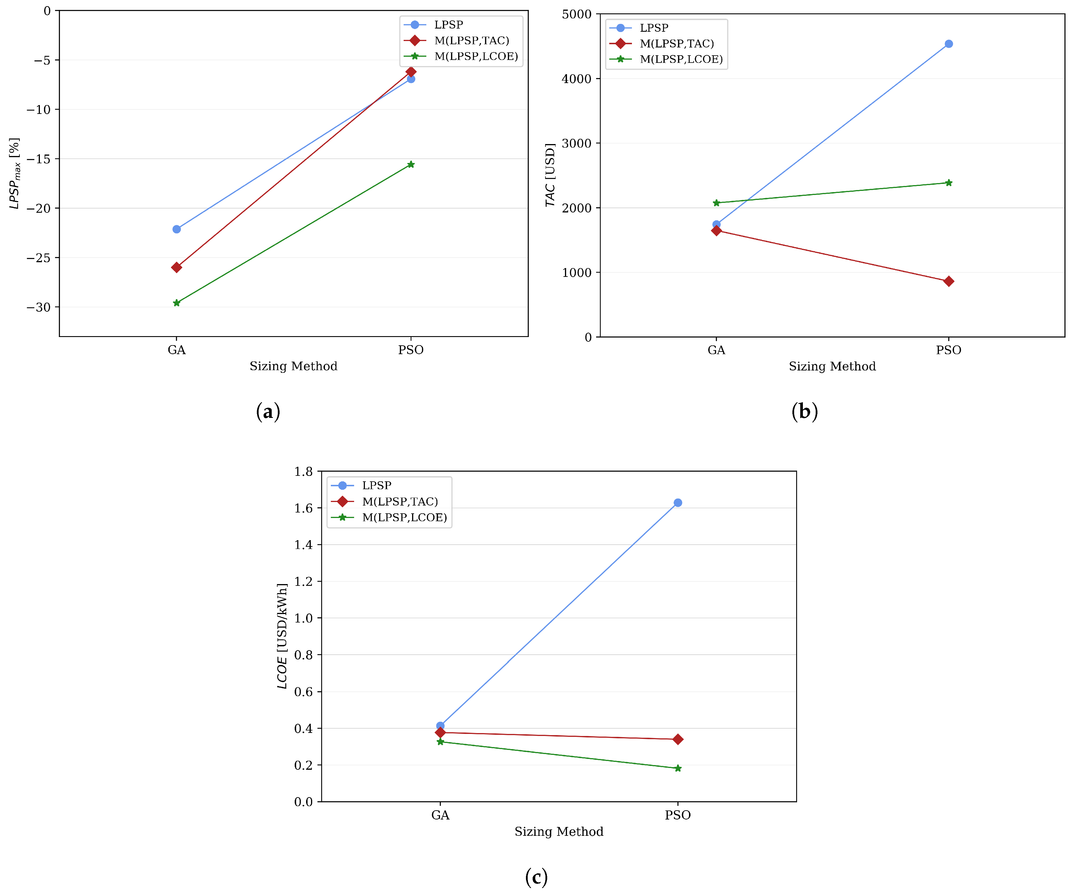
Figure 4, Figure 5 and Figure 6 show the interaction of factors on the response variables for each one of the considered demands. For the 3.6 kW-h/day demand, the values closest to zero of were obtained by minimizing the single-objective function $LPSP$; this is observed in Figure 4a. From Figure 4b, it is possible to appreciate how the minimum $TAC$ value were achieved by using the multi-objective function in terms of $LPSP$ and $TAC$, and the Figure 4c shows that the minimum $LCOE$ values were obtained by minimizing the multi-objective function of $LPSP$ and $LCOE$. This confirms that the type of objective function affects the results obtained from the hybrid renewable energy system, independently of the sizing method. Additionally, from the interactions depicted in Figure 4, the values closest to zero $LPS{P}_{max}$, obey to minimum $TAC$ and $LCOE$ values when using PSO.

Table 7. Best results for Case I: Demand of non-interconnected zone.

Simulation	${\mathit{N}}_{\mathit{wt},1}$	${\mathit{N}}_{\mathit{wt},2}$	${\mathit{N}}_{\mathit{wt},3}$	${\mathit{N}}_{\mathit{wt},4}$	${\mathit{N}}_{\mathit{pv},1}$	${\mathit{N}}_{\mathit{pv},2}$	${\mathit{N}}_{\mathit{pv},3}$	${\mathit{N}}_{\mathit{b}}$	${\mathit{L}\mathit{P}\mathit{S}\mathit{P}}_{\mathit{m}\mathit{a}\mathit{x}}$	$\mathit{T}\mathit{A}\mathit{C}$	$\mathit{L}\mathit{C}\mathit{O}\mathit{E}$
									[%]	[USD]	[USD/kW-h]
GA/LPSP	1	0	0	0	0	0	0	4	−0.007	893.98	0.583
GA/LPSP	1	0	0	0	0	0	0	9	−0.007	1044.11	0.679
GA/LPSP	1	0	0	0	0	0	0	2	−0.007	833.93	0.544
GA/M(LPSP,TAC)	0	0	0	0	6	1	0	4	−11.324	574.11	0.327
GA/M(LPSP,LCOE)	0	0	0	0	7	2	0	4	−11.338	655.35	0.264
PSO/LPSP	1	0	0	0	0	0	0	4	−0.007	893.98	0.583
PSO/LPSP	1	0	0	0	0	0	0	1	−0.007	803.90	0.524
PSO/M(LPSP,TAC)	0	0	0	0	2	1	1	4	−11.324	574.11	0.326
PSO/M(LPSP,TAC)	0	0	0	0	6	1	0	4	−11.324	574.11	0.327
PSO/M(LPSP,LCOE)	0	0	0	0	5	9	7	2	−11.032	1855.25	0.161

shows best results for the non-interconnect zone sizing system. The $LPS{P}_{max}$ value closest to zero is −0.007%, and it was obtained by minimizing the $LPSP$ function with either both sizing methods (GA and PSO), where a hybrid system composed by WT/Batteries is required with a single 1 kW wind turbine. It is observed that the number of the batteries does not affect the $LPS{P}_{max}$ value, affecting the total annual and energy cost. In this way, the best solution is composed with only one battery, achieving a $TAC$ of 803.90 USD and a $LCOE$ of 0.524 USD/kW-h by PSO.

The configuration of the HRES with the form PV/Batteries was achieved by minimizing the multi-objective function of $LPSP$ and $TAC$, both by GA and PSO, and it is characterized by including six panels of 105 W, one of 270 W and four batteries, meaning a $TAC$ of 574.11 USD at an $LCOE$ of 0.327 USD/kW-h. On the other hand, the best solution in terms of the lowest $LCOE$ value was obtained by PSO and it is composed of five panels of 105 W, 9 of 270 W, 7 of 420 W and two batteries, meaning a $TAC$ of 1855.25 USD and $LCOE$ of 0.161 USD/kW-h. The best solutions regarding the minimum $TAC$ and $LCOE$ values reached a $LPS{P}_{max}$ value of −11.324% and −11.032%, respectively. This values are higher than the obtained by the best solution of $LPSP$; therefore, the solutions based on $TAC$ and $LCOE$ have an excess of energy generation; however, these present better economic indicators. This is much more evident in the formulation of the $LCOE$, since it has the power generation in the denominator, and it is inversely proportional to the level cost of energy.

The analysis of data for the water consumption demand confirms that the minimum $TAC$ (see Figure 5b) and $LCOE$ (see Figure 5c) values were obtained by using the multi-objective function in terms of $TAC$ and $LCOE$, respectively, either through GA or PSO. There is a similarity in the minimum $LPS{P}_{max}$ value when using the PSO with the single-objective function $LPSP$ and multi-objective when integrating the total annual cost, as seen in Figure 5a. From the results presented in Figure 5, it can be observed that the PSO sizing method provides values closer to zero $LPS{P}_{max}$, with minimum $TAC$ and $LCOE$ values. The best results for an HRES sizing to supply electricity for a water consumption demand are showed in

Table 8. Best results for Case II: demand of non-interconnected zone with water consumption.

Simulation	${\mathit{N}}_{\mathit{wt},1}$	${\mathit{N}}_{\mathit{wt},2}$	${\mathit{N}}_{\mathit{wt},3}$	${\mathit{N}}_{\mathit{wt},4}$	${\mathit{N}}_{\mathit{pv},1}$	${\mathit{N}}_{\mathit{pv},2}$	${\mathit{N}}_{\mathit{pv},3}$	${\mathit{N}}_{\mathit{b}}$	${\mathit{L}\mathit{P}\mathit{S}\mathit{P}}_{\mathit{m}\mathit{a}\mathit{x}}$	$\mathit{T}\mathit{A}\mathit{C}$	$\mathit{L}\mathit{C}\mathit{O}\mathit{E}$
									[%]	[USD]	[USD/kW-h]
GA/LPSP	0	1	0	0	0	0	0	9	−0.254	1610.47	0.406
GA/LPSP	0	1	0	0	0	0	0	6	−0.254	1520.39	0.383
GA/LPSP	0	1	0	0	0	0	0	4	−0.254	1460.33	0.368
GA/LPSP	0	1	0	0	0	0	0	8	−0.254	1580.44	0.398
GA/M(LPSP,TAC)	0	0	0	0	0	0	3	4	−11.096	652.10	0.262
GA/M(LPSP,LCOE)	0	0	0	0	1	3	2	4	−11.107	759.35	0.222
PSO/LPSP	0	1	0	0	0	0	0	704	−0.254	22,479.04	6.247
PSO/M(LPSP,TAC)	0	0	0	0	6	0	1	5	−11.212	636.63	0.308
PSO/M(LPSP,TAC)	0	0	0	0	2	0	2	5	−11.212	636.63	0.308
PSO/M(LPSP,LCOE)	0	0	0	0	6	6	15	2	−6.627	2689.48	0.160

. Under the criterion of $LPS{P}_{max}$ value closer to zero, the best configuration was obtained by GA. The GA and PSO solutions consist only of a 2.1 kW wind turbine and the $LPSP$ value is independent of the size of the storage system. This is appreciable in the PSO/LPSP solution, which has 704 batteries; this is due to the fact that sizing does not involve a cost factor, and it has the freedom to search any configuration that guarantees only the energy demand.

In this way, if the solution criteria are attained for the most economical system, the best configuration achieved by GA has to be chosen, consisting of the 2.1 kW wind turbine and four batteries, taking a $TAC$ value of 1460.33 USD and a $LCOE$ of 0.368 USD/kW-h. On the other hand, two possible configurations are obtained with lower $TAC$ values by PSO, both with an annual cost value of 636.63 USD, and a $LCOE$ of 0.308 USD/kW-h; the first one integrates six panels of 105 W, one of 420 W and five batteries; the second configuration is made up of two panels of 105 W, two of 420 W, and five batteries. These two configurations share the same photo-voltaic installed capacity of 1050 W. The lowest $LCOE$ value for a HRES configuration was obtained by the PSO method, taking a value of 0.16 USD/kW-h, where the system has six panels of 105 W, 6 of 270 W, 15 of 470 W and two batteries, obtaining a total annual cost of 2689.48 USD.

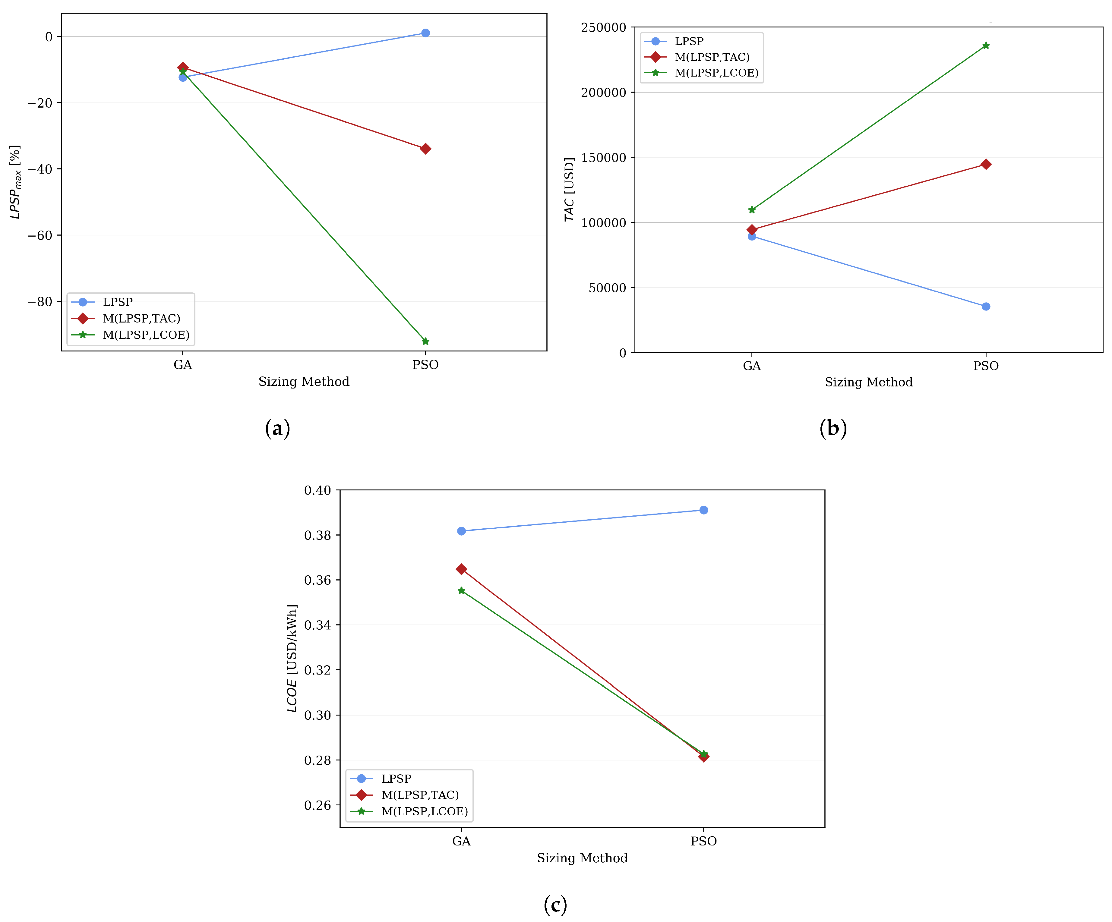
The study of a demand with a consumption of 156.15 kW-h/day shows that the value closest to zero $LPS{P}_{max}$ was obtained by minimizing the single-objective function. A similar result was obtained for the GA method for any level of the objective function (see Figure 6a). The minimum $LCOE$ value presented similar magnitudes when minimizing the multi-objective functions by $TAC$ or $LCOE$ with the PSO method, which can be seen in Figure 6c.

Unlike the other two demands, the minimum $TAC$ values were obtained when using the single-objective function $LPSP$ (see Figure 6b). This can be explained due to the fact that the search for a solution more adjusted to the demand will have less equipment integrated into the hybrid system, affecting installation, operation and maintenance costs. From the factor interaction graphs presented in Figure 6, it can be observed once again that, by means of the PSO method, it is possible to obtain values close to zero $LPS{P}_{max}$ and lower $TAC$ and $LCOE$ values.

The solutions obtained for a demand of 156.15 kW-h/day are presented in

Table 9. Best results for Case III: community demand of 156.15 kW-h/day.

Simulation	${\mathit{N}}_{\mathit{wt},1}$	${\mathit{N}}_{\mathit{wt},2}$	${\mathit{N}}_{\mathit{wt},3}$	${\mathit{N}}_{\mathit{wt},4}$	${\mathit{N}}_{\mathit{pv},1}$	${\mathit{N}}_{\mathit{pv},2}$	${\mathit{N}}_{\mathit{pv},3}$	${\mathit{N}}_{\mathit{b}}$	${\mathit{L}\mathit{P}\mathit{S}\mathit{P}}_{\mathit{m}\mathit{a}\mathit{x}}$	$\mathit{T}\mathit{A}\mathit{C}$	$\mathit{L}\mathit{C}\mathit{O}\mathit{E}$
									[%]	[USD]	[USD/kW-h]
GA/LPSP	3	17	14	1	14	3	26	105	0.280	75,896.17	0.355
GA/M(LPSP,TAC)	1	15	1	3	18	6	0	289	−12.696	42,266.63	0.413
GA/M(LPSP,LCOE)	30	42	1	3	14	5	11	36	1.067	87,156.54	0.333
PSO/LPSP	13	13	16	0	0	0	0	100	−0.009	75,560.33	0.392
PSO/LPSP	0	0	0	0	341	2	2	319	1.716	21,001.96	0.287
PSO/M(LPSP,TAC)	23	0	0	4	203	108	101	301	−12.286	64,041.62	0.253
PSO/M(LPSP,LCOE)	11	45	0	0	240	93	291	341	−6.995	126,024.73	0.236
PSO/M(LPSP,LCOE)	70	24	1	7	98	252	340	47	−0.498	166,758.36	0.236

. The configuration with a value closest to zero $LPS{P}_{max}$ was obtained with the PSO method. It is composed of 13 wind turbines of 1 kW, 13 of 2.1 kW, 16 of 5 kW, and 100 batteries. This system is characterized by having a $LPS{P}_{max}$ value of −0.009%, a $TAC$ of 75,560.33 USD, and $LCOE$ of 0.392 USD/kW-h. Similar to the analysis presented for the two previous demands, the hybrid system takes the form of WT/Batteries with a 100% fraction of wind generation. Table 9 shows the best solutions obtained in terms of the lowest $TAC$ value for the GA and PSO sizing methods when using the multi-objective function of $LPSP$ and $TAC$. However, according to Figure 6b, the minimum $TAC$ values are obtained by the PSO method with a single-objective function $LPSP$. In this sense, Table 9 also presents the best solution with a minimum $TAC$ value of 21,001.96 USD.

The HRES configuration consists in this case of 341 solar panels of 105 W, two of 270 W, two of 420 W, and 319 batteries, which achieves a loss power supply probability of 1716%. Similar to demands of 3.6 kW-h/day and 4.27 kW-h/day, the best solution in terms of the lowest total annual cost takes the form of PV/Batteries with a solar generation fraction of 100%. On the other hand, the configuration of the type WT/PV/Batteries provide the lowest $LCOE$ value through the PSO sizing, with a value of 0.236 USD/kW-h and with two possible configurations. If the economic factor is prioritized, the best solution according to $LCOE$ and at a lower total annual cost $TAC$ is characterized by 11 wind turbines of 1 kW, 45 of 2.1 kW, 240 panels of 105 W, 93 of 270 W, 291 of 470 W, and 341 batteries, representing a $TAC$ value of 126,024.73 USD and a minimum excess generation of 6.995%.

5. Discussion

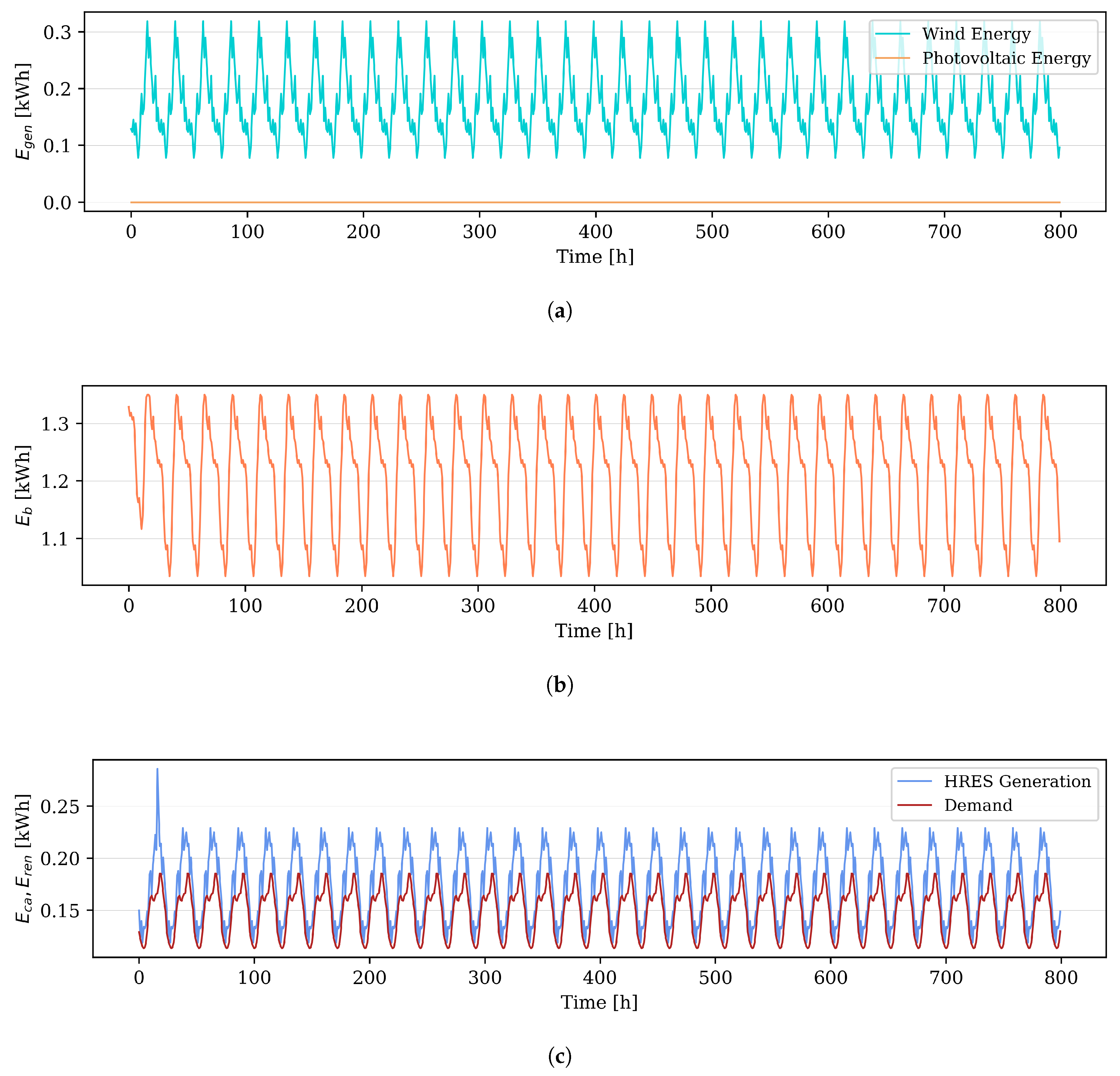
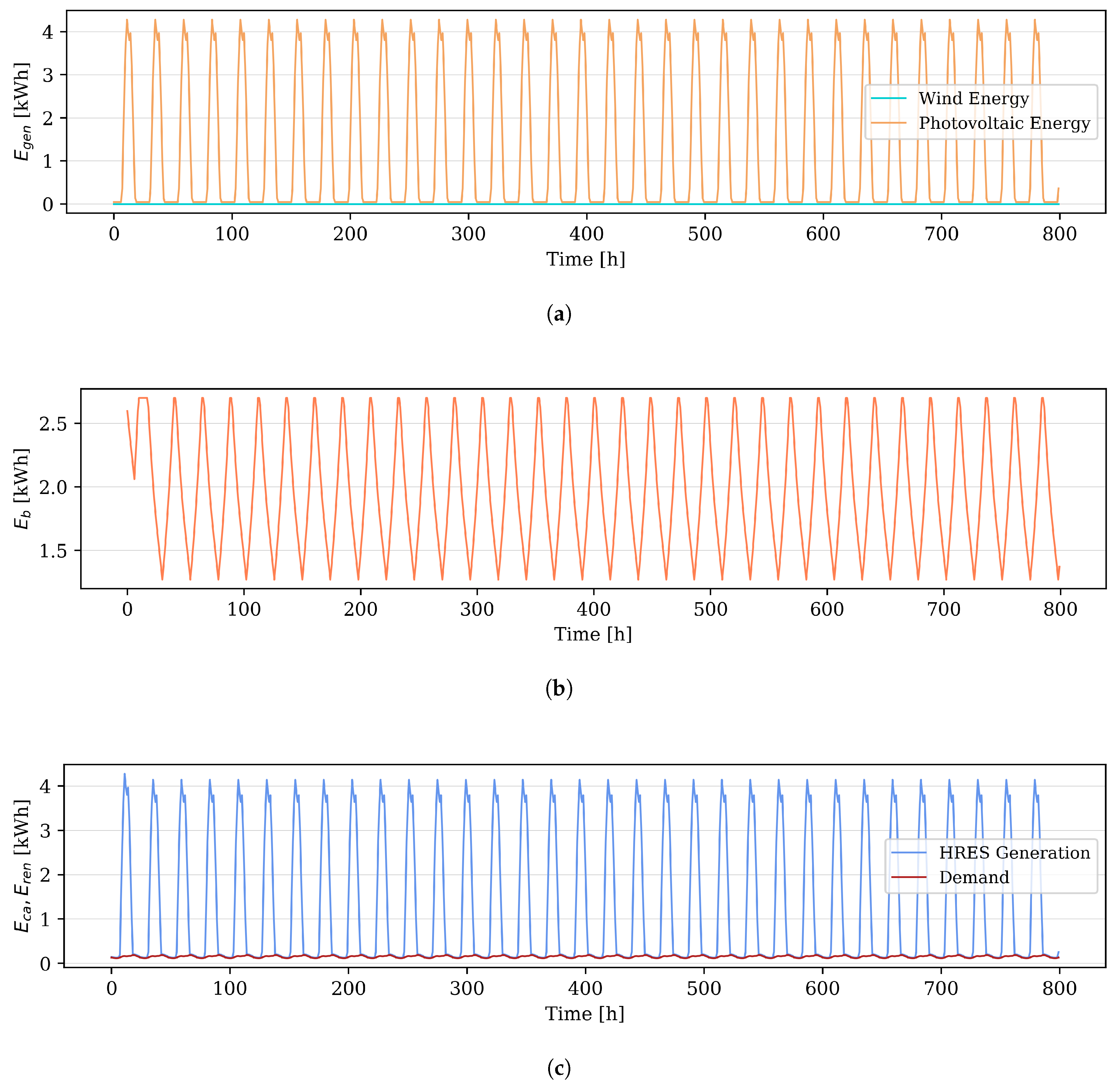
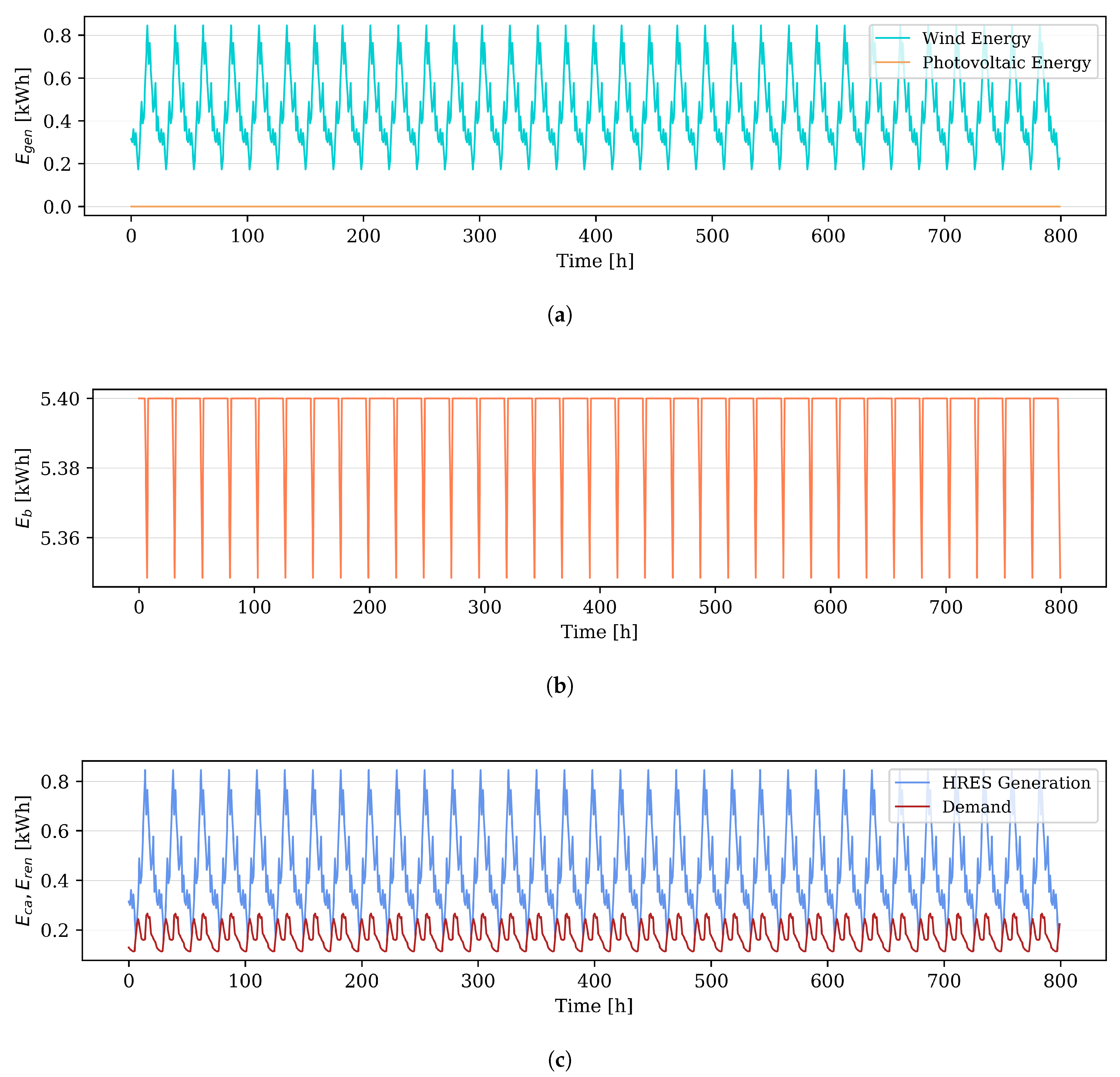
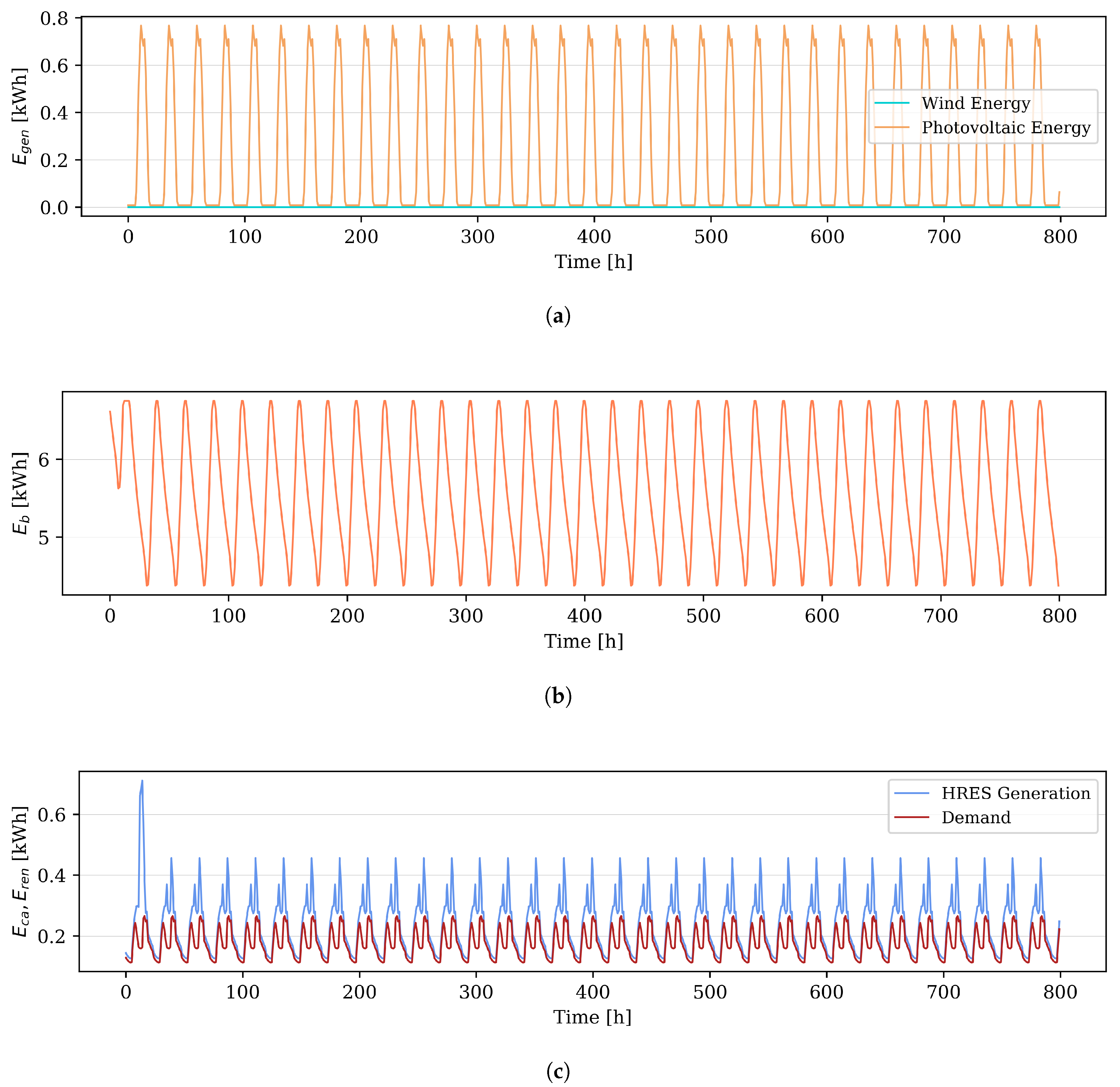
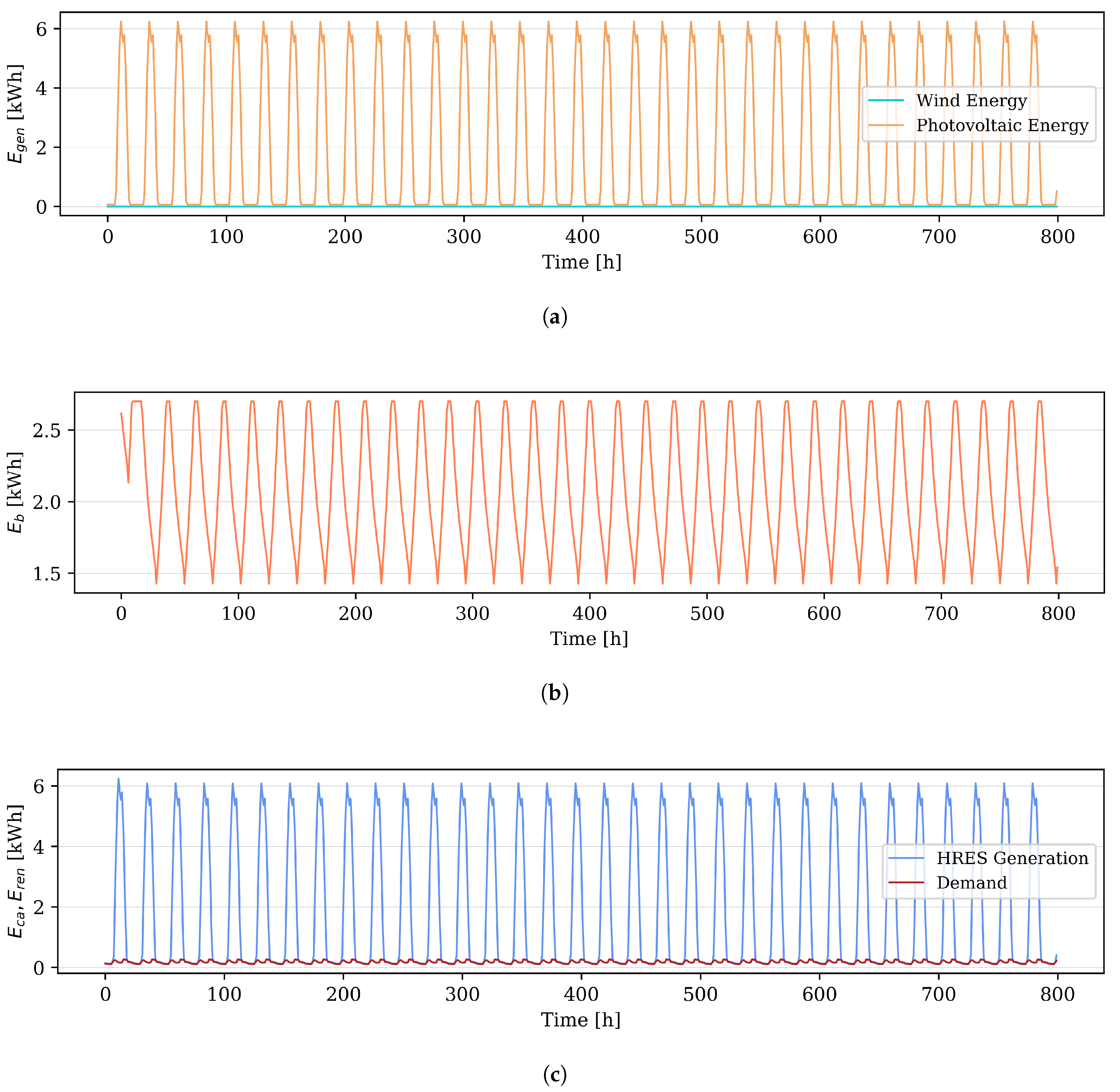
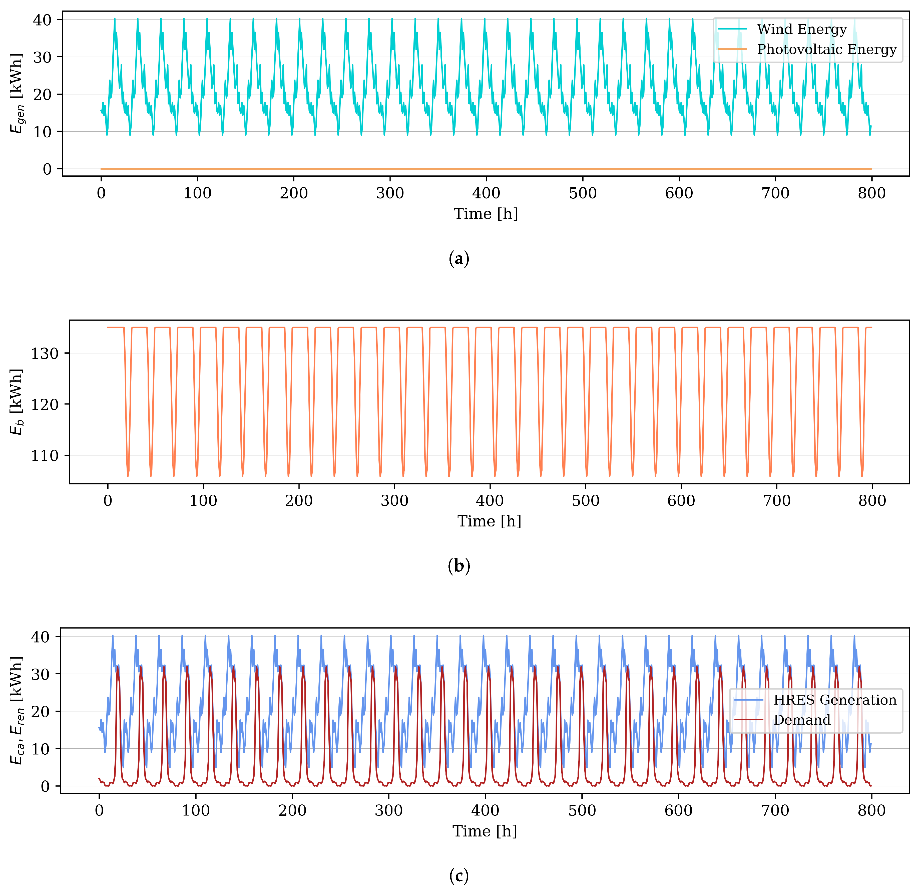
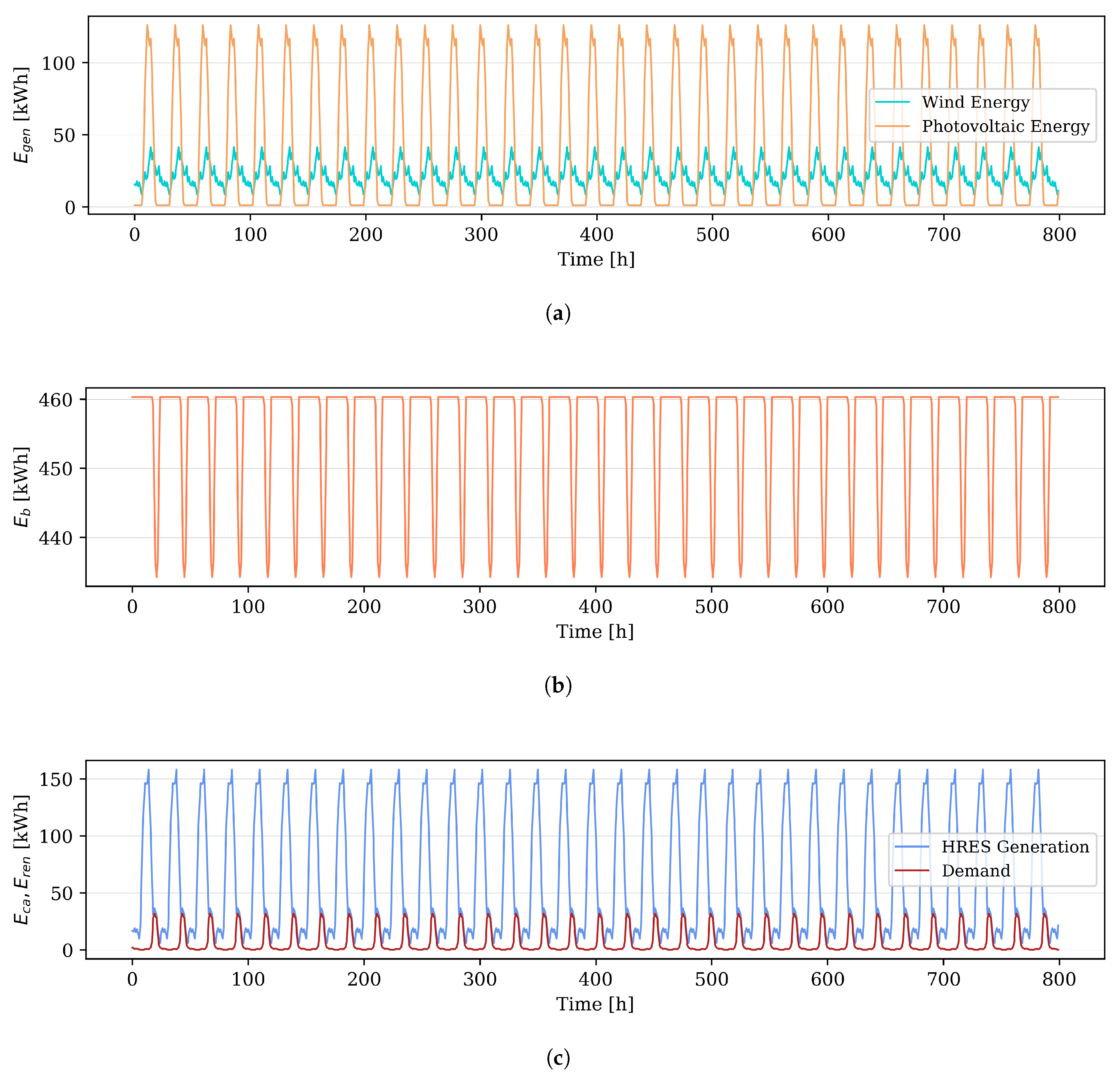
Figure A1, Figure A2, Figure A3, Figure A4, Figure A5, Figure A6, Figure A7, Figure A8 and Figure A9 present the characteristic profiles during the first 800 h of each solution. The first profile describes the total electric power generation $E_{gen}\left(t\right)$ (Equation (15)), which does not have the integration of storage system. The second profile represents the state of the storage system $E_b$ (Equations (5) and (6)) following the constraints of Equations (10)–(12). The third and last profiles compare the energy demand with the renewable system generation $E_{ren}\left(t\right)$ (Equation (16)), and it integrates the $E_{gen}\left(t\right)$ values and the state of the storage system by Equations (13) and (14).

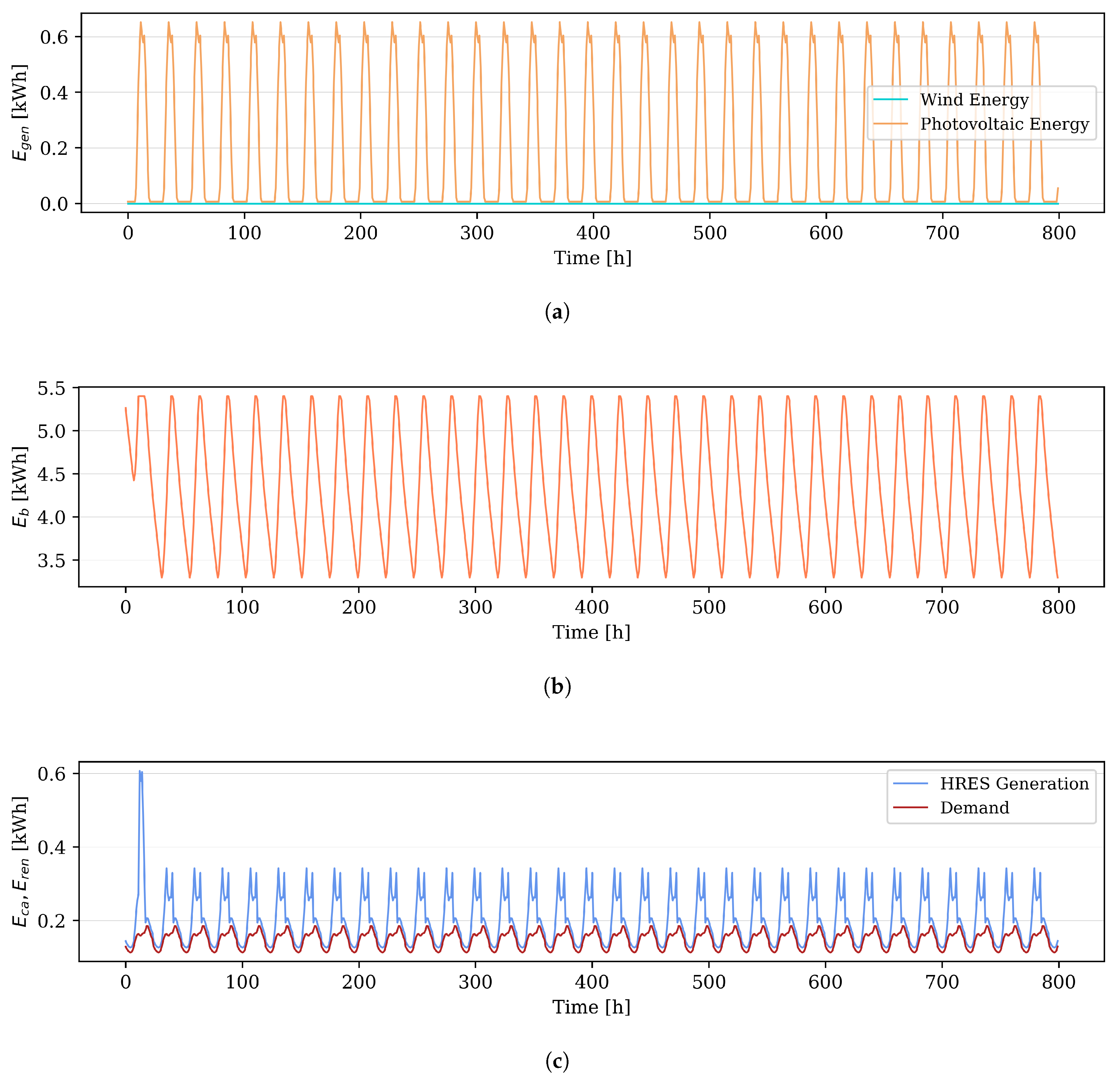
For the three demand cases, the total energy generation profile $E_{gen}\left(t\right)$ obtained by the objective function of loss power supply probability has a wind generation fraction of 100%. On the contrary, the $E_{gen}\left(t\right)$ curve for the solutions through the multi-objective function with the total annual cost have a 100% fraction of photo-voltaic generation. On the other hand, the results achieved by minimizing the multi-objective function which integrates the levelized cost of energy have a photo-voltaic fraction of 100% for the studies of non-interconnected zones and consumption of drinking water demands; however, the case of a community demand presents a hybrid system with a wind generation fraction of 28.8% and photo-voltaic fraction of 71.2%. This is represented by Figure A9a.

The state of the storage system $E_b$ for all the best configurations is characterized by presenting charge and discharge states without exceeding the maximum and minimum state restrictions. This shows that the storage system makes an energy contribution to HRES, and the wind and photo-voltaic systems generate excess energy with respect to demand, with it being possible to charge the batteries. Additionally, the renewable generation profile $E_{ren}\left(t\right)$, consistent with the curves interaction of Figure 4a, Figure 5a and Figure 6a, presents a follow-up adjusted to the demand for the solutions by minimizing $LPSP$, compared to the configurations obtained by an economic criterion ($TAC$ or $LCOE$). Therefore, the excess of generation in some operating times, despite achieving energy storage by the storage system, the maximum charge rate limits the store of the total excess energy.

According to the best solutions for each Case of demand (Table 7, Table 8 and Table 9), it is possible to infer that, when the search included the single-function by $LPSP$, the $TAC$ values reached medium magnitudes with respect to the low values obtained by multi-objectives involving the same parameter; however, higher values are reached by multi-objective relating to $LCOE$. The single-function study also showed higher $LCOE$ values than multi-objective minimization methods. Therefore, when the sizing included single-function by $LPSP$ minimization, the best configuration of HRES had $LPS{P}_{max}$ values close to zero, medium $TAC$ values, and high $LCOE$ values.

In the case of the best solutions reached by multi-objective $LPSP$ and $TAC$ evaluation, these generally showed high absolute $LPS{P}_{max}$ values in contrast with low absolute $LPS{P}_{max}$ values obtained by single-function ($LPSP$) and medium absolute $LPS{P}_{max}$ values that are reached by multi-objective relating to $LCOE$ variable. There are two exceptions, in Case I and Case II: as when the GA method is employed, results present similar absolutes $LPS{P}_{max}$ values with respect to multi-objective involving $LCOE$. Additionally, the multi-objective $LPSP$ and $TAC$ search had medium $LCOE$ values appreciate single and multi-objective relating to $LCOE$ function. In this sense, a multi-objective $LPSP$ and $TAC$ sizing meant low $TAC$ values, high absolute $LPS{P}_{max}$ values, and medium $LCOE$ values. From the above analysis, the best configurations obtained by multi-objective LCOE function show low $LCOE$ vales, medium absolute $LPS{P}_{max}$ values, and high $TAC$ values.

The study of the demand of a community with a consumption of 156.15 kW-h/day, showed that the solution with lower $TAC$ value is obtained by the single-objective function $LPSP$. This is justified by the fact that, if a system is more adjusted to demand, it also reduces the amount of equipment needed for the operation and the total annual cost. Note that the particular solution for this demand has an $LPS{P}_{max}$ value greater than zero (1.716%), compared to other particular configurations described in this paper. It can be inferred that it is possible to sacrifice the reliability of the system, in order to achieve lower annual cost values. In this way, despite the fact that the best particular solution for 156.15 kW-h/day demand presents an $LPS{P}_{max}$ value of 1.716%, it can also take negative values of $LPSP$ for other time periods, which means excess power generation, as showed in Figure A8c.

The best particular solution for the demand with water consumption, obtained by single-objective function of $LPSP$, was achieved by the GA method, and not by PSO as evidenced in the factor interaction of Figure 5a. This is due to statistical experimental design being performed with several results (25 results for each factor interaction); therefore, the factors interaction provide a general view of the resulting configurations, while the best solution was chosen according to the minimum $TAC$ value, which represents an outlier with respect to the total results sample.

6. Conclusions

This paper justifies the use of hybrid renewable energy systems (HRES) in the Colombian context, specifically for the region of Puerto Bolívar, La Guajira, which is a representative zone due to its outstanding wind and solar resources. The results obtained were evaluated according to the factors interaction methodology provided by an experimental design—considering the results’ dependency on the setup parameters for the implementation of the sizing methods, inferred through a sample evaluation of twenty-five possible configurations for each Case of interaction between factors.

The configuration of an HRES of the form WT/Batteries with 100% wind generation fraction was obtained by sizing with the objective function of $LPSP$. In contrast, a system of the form PV/Batteries predominates in the solutions where the search is based on economic factors, like $TAC$ or $LCOE$.

The PSO sizing method provides solutions that are more adjusted to demand, with lower annual costs or lower levelized costs of energy, depending on the type of objective function. The search for loss power supply probability ($LPSP$) yields configurations more adjusted to the energy demand; this is represented by values of $LPS{P}_{max}$ close to zero. When the method minimizes the multi-objective function with $LPSP$ and $TAC$, configurations with low total annual costs are obtained. On the other hand, the evaluation of the multi-function objective with $LPSP$ and $LCOE$, generates configurations with lower values of the level cost of energy $LCOE$, which are characterized by low total annual costs or high energy generation (by formulation).

A system obtained by minimizing $LPSP$ follows the demand profile with its generation of renewable energy, while an HRES obtained by economic criteria presents excess energy that the storage system can not store totally, due to the restriction of the maximum charge rate. This generation excess could be used to feed an additional demand, such as the energy for operating a system that coincides with the specific time instants where the generation exceeds the initial demand considered, or takes advantage of the integration with the transmission grid, following the technical, economic, and political guidelines of the region.

The genetic algorithm and particle swarm optimization can be used for the techno-economic sizing of a HRES and its implementation in the Colombian context. The PSO method achieves the best technical or economic indicators, depending on the type of objective function and the design criteria; however, the GA method can obtain outlier solutions that meet the reliability and cost values.

References

1. Paredes, J.R.; Ramírez, J.J. Variable Renewable Energies and Their Contribution to Energy Security: Complementarity in Colombia; Banco Interamericano de Desarrollo: Washington, DC, USA, 2017; p. 59. [Google Scholar]
2. Ahmad, T.; Zhang, D. A critical review of comparative global historical energy consumption and future demand: The story told so far. Energy Rep. 2020, 6, 1973–1991. [Google Scholar] [CrossRef]
3. UPME. Integración de las Energías Renovables no Convencionales en Colombia Integración de las Energías en Colombia; UPME: Bogota, Colombia, 2015.
4. International Renewable Energy Agency. IRENA (2019), Global Energy Transformation: A Roadmap to 2050; International Renewable Energy Agency: Abu Dhabi, UAE, 2019; pp. 52 (10–23). [Google Scholar]
5. Unidad de Planeación Minero Energética; UPME. Informe de Gestión 2018. 2018. Available online: http://www1.upme.gov.co/InformesGestion/Informe{_}de{_}gestion{_}2018{_}19092018.pdf (accessed on 14 September 2020).
6. Superintendencia Delegada para Energía y Gas Combustible. Zonas No Interconectadas—ZNI Diagnóstico de la Prestación del Servicio de Energía Eléctrica 2017. 2017. Available online: https://www.superservicios.gov.co/sites/default/archivos/SSPDPublicaciones/Publicaciones/2018/Sep/diagnosticozni-superservicios-oct-2017.pdf (accessed on 14 September 2020).
7. Instituto de Hidrología Meteorología y Estudios Ambientales; IDEAM. Consulta y Descarga de Datos Hidrometeorológicos. 2017. Available online: http://dhime.ideam.gov.co/atencionciudadano/ (accessed on 5 January 2019).
8. Observatorio de Minas y Energía; UPME. Precios Paises Comparables. 2019. Available online: https://www1.upme.gov.co/InformacionCifras/Paginas/precios-energia-electrica-comparacion-paises.aspx (accessed on 14 September 2020).
9. Superintendencia Delegada para Energía y Gas Combustible. Zonas No Interconectadas—ZNI Diagnóstico de la Prestación del Servicio de Energía Eléctrica 2018. 2018. Available online: https://www.superservicios.gov.co/publicaciones/energia-y-gas/ (accessed on 25 September 2020).
10. Miao, C.; Teng, K.; Wang, Y.; Jiang, L. Technoeconomic Analysis on a Hybrid Power System for the UK Household Using Renewable Energy: A Case Study. Energies 2020, 13, 3231. [Google Scholar] [CrossRef]
11. The International Renewable Energy Agency; IRENA. Renewable Power Generation Costs in 2017. 2017. Available online: https://www.irena.org/publications/2018/Jan/Renewable-power-generation-costs-in-2017 (accessed on 14 September 2020).
12. Jouhara, H.; Serey, N.; Khordehgah, N.; Bennett, R.; Almahmoud, S.; Lester, S.P. Investigation, development and experimental analyses of a heat pipe based battery thermal management system. Int. J. Thermofluids 2020, 1–2, 100004. [Google Scholar] [CrossRef]
13. Mahmoudimehr, J.; Shabani, M. Optimal design of hybrid photovoltaic-hydroelectric standalone energy system for north and south of Iran. Renew. Energy 2018, 115, 238–251. [Google Scholar] [CrossRef]
14. Khordehgah, N. Latent Thermal Energy Storage Technologies and Applications: A Review. Int. J. Thermofluids 2020, 6, 100039. [Google Scholar] [CrossRef]
15. Bhandari, B.; Poudel, S.R.; Lee, K.T.; Ahn, S.H. Mathematical modeling of hybrid renewable energy system: A review on small hydro-solar-wind power generation. Int. J. Precis. Eng. Manuf. Green Technol. 2014, 1, 157–173. [Google Scholar] [CrossRef]
16. Koutroulis, E.; Kolokotsa, D.; Potirakis, A.; Kalaitzakis, K. Methodology for optimal sizing of stand-alone photovoltaic/wind-generator systems using genetic algorithms. Sol. Energy 2006, 80, 1072–1088. [Google Scholar] [CrossRef]
17. Twaha, S.; Ramli, M.A. A review of optimization approaches for hybrid distributed energy generation systems: Off-grid and grid-connected systems. Sustain. Cities Soc. 2018, 41, 1–19. [Google Scholar] [CrossRef]
18. Askarzadeh, A. A novel metaheuristic method for solving constrained engineering optimization problems: Crow search algorithm. Comput. Struct. 2016, 169, 1–12. [Google Scholar] [CrossRef]
19. Khare, V.; Nema, S.; Baredar, P. Solar-wind hybrid renewable energy system: A review. Renew. Sustain. Energy Rev. 2016, 58, 23–33. [Google Scholar] [CrossRef]
20. Tito, S.R.; Lie, T.T.; Anderson, T.N. Optimal sizing of a wind-photovoltaic-battery hybrid renewable energy system considering socio-demographic factors. Sol. Energy 2016, 136, 525–532. [Google Scholar] [CrossRef] [Green Version]
21. Khatib, T.; Mohamed, A.; Sopian, K. Optimization of a PV/wind micro-grid for rural housing electrification using a hybrid iterative/genetic algorithm: Case study of Kuala Terengganu, Malaysia. Energy Build. 2012, 47, 321–331. [Google Scholar] [CrossRef]
22. Kamjoo, A.; Maheri, A.; Dizqah, A.M.; Putrus, G.A. Multi-objective design under uncertainties of hybrid renewable energy system using NSGA-II and chance constrained programming. Int. J. Electr. Power Energy Syst. 2016, 74, 187–194. [Google Scholar] [CrossRef]
23. Merei, G.; Berger, C.; Sauer, D.U. Optimization of an off-grid hybrid PV-Wind-Diesel system with different battery technologies using genetic algorithm. Sol. Energy 2013, 97, 460–473. [Google Scholar] [CrossRef]
24. Borhanazad, H.; Mekhilef, S.; Gounder Ganapathy, V.; Modiri-Delshad, M.; Mirtaheri, A. Optimization of micro-grid system using MOPSO. Renew. Energy 2014, 71, 295–306. [Google Scholar] [CrossRef]
25. Barrozo-Budes, F.A.; Valencia Ochoa, G.; Obregon, L.G.; Arango-Manrique, A.; Núñez Álvarez, J.R. Energy, Economic, and Environmental Evaluation of a Proposed Solar-Wind Power On-grid System Using HOMER Pro®: A Case Study in Colombia. Energies 2020, 13, 1662. [Google Scholar] [CrossRef]
26. World Energy Council. Energy Trilemma Index. 2019. Available online: https://www.worldenergy.org/transition-toolkit/world-energy-trilemma-index (accessed on 14 September 2020).
27. Woolmington, T.; Sunderland, K.; Blackledge, J.; Conlon, M. The progressive development of turbulence statistics and its impact on wind power predictability. Energy 2014, 77, 25–34. [Google Scholar] [CrossRef] [Green Version]
28. Maleki, A.; Pourfayaz, F. Optimal sizing of autonomous hybrid photovoltaic/wind/battery power system with LPSP technology by using evolutionary algorithms. Sol. Energy 2015, 115, 471–483. [Google Scholar] [CrossRef]
29. Malheiro, A.; Castro, P.M.; Lima, R.M.; Estanqueiro, A. Integrated sizing and scheduling of wind/PV/diesel/battery isolated systems. Renew. Energy 2015, 83, 646–657. [Google Scholar] [CrossRef] [Green Version]
30. HOMER Energy LLC. HOMER PRO. 2019. Available online: https://www.homerenergy.com/ (accessed on 14 September 2020).
31. Domínguez, E.A.; Rivera, H.G.; Vanegas, R.; Moreno, P. Relaciones demanda-oferta de agua y el índice de escasez de agua como herramientas de evaluación del recurso hídrico colombiano. Rev. Acad. Colomb. Cienc. 2008, 32, 195–212. Available online: https://raccefyn.co/index.php/raccefyn/issue/view/173 (accessed on 27 October 2020).
32. Jarramillo, O.; Gonzales, M.; Saldarriaga, G. Conceptualización y dimensionamiento de la demanda hídrica sectorial. Gestión y Ambiente 2010, 81–92. [Google Scholar] [CrossRef] [Green Version]
33. Cisse, O.; Nkounga, W.M.; NDIAYE, M.F.; Ndiaye, P.A. Water and Energy Management based on Fuzzy Logic and Linear Programming for a Photovoltaic Wind/Battery Pumping System in Rural Environment. In Proceedings of the 7th International Conference on Renewable Energy Research and Applications, Paris, France, 14–17 October 2018; Volume 5, pp. 3–8. [Google Scholar]
34. Muhsen, D.H.; Khatib, T.; Nagi, F. A review of photovoltaic water pumping system designing methods, control strategies and field performance. Renew. Sustain. Energy Rev. 2017, 68, 70–86. [Google Scholar] [CrossRef]
35. Wakeel, M.; Chen, B.; Hayat, T.; Alsaedi, A.; Ahmad, B. Energy consumption for water use cycles in different countries: A review. Appl. Energy 2016, 178, 868–885. [Google Scholar] [CrossRef]
36. Jain, R.; Camarillo, M.K.; Stringfellow, W.T. (Eds.) Chapter 3—Threats. In Drinking Water Security for Engineers, Planners, and Managers; Butterworth-Heinemann: Boston, MA, USA, 2014; pp. 45–67. [Google Scholar] [CrossRef]
37. IPSE. Instituto de Planeación y Promoción de Soluciones Energéticas para las Zonas No Interconectadas. 2019. Available online: http://190.216.196.84/cnm/no_telemetria.php?v1=REPORTE%20GERENCIAL%20ENE%20DIC%202018.pdf (accessed on 14 September 2020).
38. IPSE. Informe Telemetría Mensual de Diciembre 2019. 2020. Available online: http://190.216.196.84/cnm/Data/info_operacion/2019/12-informemensualdiciembre2019.rar (accessed on 14 September 2020).
39. Aelos. Aeolos Wind Turbine 1kW Specification. 2020. Available online: https://www.windturbinestar.com/1kwh.html (accessed on 14 September 2020).
40. Renugen. Aeolos Aeolos-H 1kW 1kW Wind Turbine. 2020. Available online: https://www.renugen.co.uk/aeolos-aeolos-h-1kw-1kw-wind-turbine/ (accessed on 14 September 2020).
41. Small Wind Certification Council. Xzeres Skystream 3.7 SWCC Summary Report; Technical Report; Small Wind Certification Council: Brea, CA, USA, 2019; Available online: http://smallwindcertification.org/certified-turbines/skystream-3-7 (accessed on 27 October 2020).
42. Bornay. Wind+. 2020. Available online: https://www.bornay.com/es/productos/aerogeneradores/wind-plus (accessed on 14 September 2020).
43. Small Wind Certification Council. Endurance S-343 SWCC Summary Report; Technical Report; Small Wind Certification Council: Brea, CA, USA, 2014; Available online: http://smallwindcertification.org/certified-turbines/endurance-s-343 (accessed on 23 December 2019).
44. Rodriguez-Hernandez, O.; Martinez, M.; Lopez-Villalobos, C.; Garcia, H.; Campos-Amezcua, R. Techno-economic feasibility study of small wind turbines in the Valley of Mexico metropolitan area. Energies 2019, 12, 890. [Google Scholar] [CrossRef] [Green Version]
45. FirstSolar. Series 4 PV Module. 2014. Available online: http://www.firstsolar.com/-/media/First-Solar/Technical-Documents/Series-4-Datasheets/Series-4V3-Module-Datasheet.ashx (accessed on 14 September 2020).
46. Ecodelta. Products & Technology. 2020. Available online: http://www.ecodeltapower.com/products{_}class{_}2.html (accessed on 14 September 2020).
47. FirstSolar. Series 6 PV Module. 2018. Available online: http://www.firstsolar.com/-/media/First-Solar/Technical-Documents/Series-6-Datasheets/Series-6-Datasheet.ashx (accessed on 14 September 2020).
48. Fu, R.; Feldman, D.; Margolis, R. U.S. Solar Photovoltaic System Cost Benchmark: Q1 2018. Nrel 2018, 1–47. [Google Scholar] [CrossRef]
49. van Rossum, G. Python Tutorial, Technical Report CS-R9526; Centrum voor Wiskunde en Informatica (CWI): Amsterdam, The Netherlands, 1995; pp. 1–65. [Google Scholar]
50. Maleki, A.; Askarzadeh, A. Comparative study of artificial intelligence techniques for sizing of a hydrogen-based stand-alone photovoltaic/wind hybrid system. Int. J. Hydrogen Energy 2014, 39, 9973–9984. [Google Scholar] [CrossRef]
51. Montgomery, D.C. Design and Analysis of Experiments, 8th ed.; John Wiley & Sons, Inc.: Hoboken, NJ, USA, 2012. [Google Scholar] [CrossRef]
Figure 1. Natural resource profiles in one day in Puerto Bolivar, La Guajira, Colombia [7]. (a) Wind speed. (b) Solar radiation and temperature.
Energies 13 05648 g001
Figure 2. Demand profiles.
Energies 13 05648 g002
Figure 3. Sizing methods flow charts. (a) Genetic Algorithm GA. (b) Particle Swarm Optimization PSO.
Energies 13 05648 g003
Figure 4. Interaction factors for Case I: demand of non-interconnected zone demand. (a) L P S P m a x (b) TAC (c) LCOE.
Energies 13 05648 g004
Figure 5. Interaction factors for Case II: demand of non-interconnected zone with water consumption. (a) L P S P m a x (b) TAC (c) LCOE.
Energies 13 05648 g005
Figure 6. Interaction factors for Case III: community demand of 156.15 kW-h/day. (a) L P S P m a x (b) TAC (c) LCOE.
Energies 13 05648 g006