Article

The Impact of Industry on European Union Emissions Trading Market—From Network Perspective

1
College of Management and Economics, Tianjin University, Tianjin 300072, China
2
Institutes of Science and Development, Chinese Academy of Sciences, Beijing 100190, China
3
School of Economics & Management, Beihang University, Beijing 100191, China
*
Author to whom correspondence should be addressed.
Energies 2020, 13(21), 5642; https://doi.org/10.3390/en13215642
Submission received: 14 September 2020 / Revised: 23 October 2020 / Accepted: 26 October 2020 / Published: 28 October 2020
(This article belongs to the Special Issue Solutions to Climate Emergency)

Abstract

:
This study pioneers to investigate the impact of industry on the European Union carbon trading market based on network perspective. All the accounts in the European Union Emissions Trading System (EU ETS) are summarized at the industry level, and then the trading relationship between industries is constructed in the network layout. Based on this network, the centrality of each industry is measured—the industries of electricity, gas, steam and air conditioning supply (EGSAS), bank, broker, exchange, and wholesale trade excluding motor vehicles and motorcycles (WTEM) have higher centrality. Finally, the impact of industry on the evolution of networks is analyzed, Findings show that the financial intermediaries play important roles at the beginning of each phase, while their influences on the network will decrease as the market goes on. On the contrary, influences of some other industries like WTEM are gradually increasing.

Graphical Abstract

1. Introduction

The European Union Emissions Trading System (EU ETS) was established in 2005, and it is the first and largest carbon emission trading market in the world by far. The goal of the system is to use market mechanisms to effectively control carbon emissions within the EU. In order to continuously optimize the system mechanism, the development of EU ETS is divided into four phases by the designer. The first phase, from 2005 to 2007, is a phase of “learning by doing”, so it is also called the pilot phase of EU ETS; the second phase, from 2008 to 2012; the third phase, from 2013 to 2020; and the fourth phase from 2021 to 2030. Since the implementation of EU ETS, the transboundary cap-and-trade scheme has been a hot topic for governments and researchers. It provides inspiration for emissions reduction in a fresh dimension, and similar ETSs were established in many regions from then, including China, Japan, Alberta and Quebec in Canada, California in the western part of the US, Kazakhstan, South Korea.
In recent years, the volume of literature on the EU ETS has been growing rapidly, and most of the study can be divided into five categories: (i) Emissions abatement under the EU ETS [1,2,3]; (ii) the operating mechanism of the ETS, including the allocation mechanism of the carbon allowances [4,5,6] and the pricing mechanism in the trading system [7,8]; (iii) the economic effect of the EU ETS, mainly including the following aspects—the influences of EU ETS on the power generation and emission reduction technology investment of energy industry [9,10], the influences of EU ETS on the operation of aviation sector [11], and industrial production sectors [12,13,14]; (iv) the effects of EU ETS on the competitiveness of regulated firms [15,16], and findings that EU ETS does not affect firms’ competitiveness significantly; (v) the influences of macro-economic on the carbon price. Results showed that the carbon futures market had only a very weak relation with the macro-economy, and the macro-economy change could not predict the volatility of the carbon futures market [16,17].
The three types of literature mentioned above focus predominantly on the carbon price in the EU ETS. However, little attention has been paid to the trading behaviors, due to the difficulty of data capture in the EU ETS. Moreover, some studies analyze the ETS in terms of participants’ trading behaviors in the trading market. Very few studies are dedicated to a detailed analysis of the transactions data set in the EU ETS. Among them, Betz and Schmidt [18] analyze the transfer patterns in Phase I of EU ETS at the account level, and they find that most installations’ accounts do not actively participate in the trading market, while the accounts belonging to intermediaries are more active. This finding is consistent with the survey analysis which shows the limited participation to the EU ETS [19,20]. As different types of accounts have different participation in the trading market, in order to identify the impacts of different trading patterns in the EU ETS, Fan [21] and Wang [22] divide transactions into three categories: Speculative trading of intermediaries’ accounts, compliance trading that intends to fill emitting accounts’ positions, and non-compliance trading that intends to increase emitting accounts’ positions. Jaraite et al. [23,24] map individual accounts in EU ETS to their parent company. Based on the mapping work, Liu [19] analyzes the different efforts in increasing profits and saving costs during the allowances trading among energy sector, manufacturing sector, and other sectors, while Cludius and Betz [25] focus on the roles of different types of intermediations like bank, broker, and exchange.
The data analysis of trading behaviors can better show the performances of some specific groups. However, the trading structure of EU ETS cannot be well displayed. Therefore, some network analysis is applied to the study of the carbon trading market. Karpf et al. [26] establish a trading network based on the accounts level, and the informational asymmetries are represented by the density in the network. They find that the informational asymmetries have dynamic influences on the gap between ask and bid price: when the informational asymmetries increase, the gap between ask and bid price increases, and when the information asymmetry decreases, the gap of that decreases. The insufficiency lies in that there are many accounts belonging to the same company, so, there are lots of inner transactions within the company, and the measurement of network density is seriously affected. The trading network analysis at the country level can avoid the existence of the inner transaction in the same company [27,28]. However, as Betz and Schmidt [18] have argued, companies can strategically choose to open another account in another country, and since it is difficult to track the nationality of an account’s owner, it is worth considering whether it is significant to study the trading network from country level.
To make up for the shortcomings of the above-mentioned in the research of EU ETS, this paper establishes a trading network of EU ETS in Phase I and Phase II at the industry level, and as the finding of Cludius and Betz [25] show, companies tend to make transactions within the same industry. Based on the trading network, the trading volume among industries can be calculated and the trading relationships are revealed. Then, the centralities of each industry in the trading market are evaluated through the trading network. Moreover, the indexes of network density, max strongly connected graph, and average shortest path are used to measure the evolution of the trading network in Phase I and Phase II. Finally, based on the centrality analysis, the industries that have higher centrality are identified, and their dynamic influences on the trading network are studied in Phase I and Phase II, respectively.
The contribution of this network analysis for EU trading market has two aspects. In terms of literature research, this research studies the trading structure from network perspective at a micro level and fills the gaps in the literature about EU ETS. Due to the difficulty in acquisition of full-sample trading data, few researches which study the trading relationship are mainly conducted at the country level [27]. In this study, based on multiple datasets, the full sample of transaction data within account level are summarized to company level and then to the industry level. Therefore, the network analysis can reveal the evolution of trading structure from industry level intuitionally. In terms of practical application, the findings in this study will help market managers make a variety of market policies in different periods of a phase for different industries. Because according to the analyses of network structure evolution, the role changes of each industry in a whole phase can be known, especially the industries with large volume transactions, like electricity, gas, steam, and air conditioning supply (EGSAS), bank, broker, and exchange.
The structure of this article is as follows: Chapter 2 introduces the sources of trading data in EU ETS; Chapter 3 introduces the process of constructing the trading network and the network indexes; Chapter 4 shows the results of the network analysis; Chapter 5 includes the conclusion; and Chapter 6 shows the research outlook.

2. Data

The transaction records of EU ETS are recorded and published by the Community Independent Transaction Log (CITL), which records detailed information of the issuance, retirement, allocation, surrender, cancellation, trading, and other operations (https://ec.europa.eu/clima/ets/). In the dataset of CITL, the allowance circulation of allowances is recorded at the account level. The transaction data can be downloaded and viewed from the EU Commission’s website, while the publication has a three-year lag. Up to now, the EU ETS is still operating in Phase III, and many emitting companies used to fulfill the gap their allowances position in the end of phase, indicating that it is not very meaningful to analyze the trading structure of the first half of Phase III separately. Therefore, this study will focus on the study of trading data in the complete first two phases.
To analyze the trading dataset from the industry level, the accounts information needs to be aggregated to company level and then industry level. The “Ownership Links and Enhanced EUTL2 Dataset” project is the unique ownership link [23,24] that aims at aggregating the account information to company level, so the owner company of each account can be found. Cludius and Betz [25] further improve this work and enable it to link all active accounts to their parent companies. Moreover, the industry classification of the industry is also provided in their work. Based on the work of Jaraite et al. and Betz [25], we can summarize all the account information to industry level. The description of each industry is shown as below:
  • EGSAS: Electricity, gas, steam, and air conditioning supply.
  • WTEM: Wholesale trade, excluding motor vehicles and motorcycles.
  • MONM: Manufacture of other non-metallic mineral products.
  • MBM: Manufacture of basic metals.
  • MCRP: Manufacture of coke and refined petroleum products.
  • MCC: Manufacture of chemicals and chemical products.
  • OOOB: Office administrative, office support, and other business support activities.
  • PADC: Public administration and defense; compulsory social security.
  • MPP: Manufacture of paper and paper products.
  • AHMC: Activities of head offices; management consultancy activities.
  • MF: Manufacture of food products.
  • ECP: Extraction of crude petroleum.
  • OPST: Other professional, scientific, and technical activities.
  • AETA: Architectural and engineering activities; technical testing and analysis
  • MMTS: Manufacture of motor vehicles, trailers, and semi-trailers
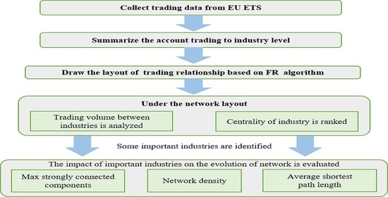
3. Methods

3.1. Network Construction

In this study of EU ETS, the allowances trading among accounts are summarized to industry level, therefore the records of intra-industry transactions are removed, and the transactions between different industries are retained. The directed networks of allowances trading in Phase I and Phase II are established through the software of ‘Gephi’. The industries are represented by nodes in the networks, and there will be a directed edge between two nodes if they have any transactions in a whole phase, with the direction of the edge symbolizing the direction of allowances flow. The edges can be two-way if the connected nodes have transactions in different directions. To better show the trading structure in EU ETS, the Fruchterman–Reingold (FR) [29] algorithm is applied to draw the networks.
Force-directed layout was first proposed by Peter Eades [30] in 1984. The purpose is to reduce the intersection of edges in the layout and try to keep the length consistent with the edges. This method uses a spring model to simulate the process of forming layout. After the action of the elastic force, the points that are too close will be bounced away and the points that are too far are pulled closer; through continuous iteration, the entire layout achieves dynamic equilibrium and tends to be stable.
After the force-guided layout was proposed, many scholars made improvements on this basis. The most typical algorithm is the FR algorithm, as it is easier to understand and implement, and can be used for most network data sets. The achieved layout has good symmetry and local aggregation, so it is more beautiful. FR algorithm is based on the theory of particle physics, which simulates nodes as atoms, and calculates positional relationship between nodes by simulating the force field of the atoms. Each iteration of the model is mainly divided into three parts: first, calculating the repulsive force between unconnected nodes, then calculating the attractive force between connected points, and finally combining the attractive force and repulsive force to determine the relative position of the nodes.
FR algorithm is defined as follows:
a r e a = W × H
where a r e a is the area of the layout, W and H are the width and height of the layout.
k = a r e a | V |
where k is the balance distance, also called the ideal distance, and |V| is the number of nodes in the layout.
d i s t ( u ,   v ) = ( u .   p o s x v .   p o s x ) 2 + ( u .   p o s y v .   p o s y ) 2
where d i s t ( u ,   v ) is the geometric distance between nodes.
f α ( u , v ) = ( d i s ( u , v ) ) 2 / k
where f α ( u , v ) is the attraction function between u and v.
f r ( u , v ) = k 2 / d i s t ( u , v )
where f r ( u , v ) is the repulsion function between u and v.

3.2. Network Indexes

The forming of trading network in the EU ETS is a long process. In the beginning of a phase, there are only a few nodes and edges appearing in the network, as only a small number of industries make transactions. As time goes by, there are more and more industries making transactions, with more and more nodes and edges appearing in the network. In this study, the analysis is implemented through the package of ‘NetworkX’ in Python 3, and some dynamic indexes in the package are selected to evaluate the evolution of trading network, where the time interval is day.
Degree centrality: The number of other industries that are directly connected to a certain industry. If an industry is directly connected to many industries, then the industry has a higher degree of centrality. Since this measurement only focuses on the number of points directly connected to a certain industry and ignores the number of indirectly connected industries, it is regarded as local centrality.
C d e g ( u ) = d u | V | 1
where d u is the number of nodes that connected to the node u.
Betweenness centrality: It measures the possibility that an industry can become a “middleman”, that is, the ability to control information transmission.
C b t w ( u ) = s , t V σ s , t ( u ) σ s , t
where σ s , t is the number of shortest ways from node s to node t, σ s , t ( u ) is the number of the number of shortest ways from node s to node t which via node u, and V is the set of nodes in the network.
Closeness centrality: The reciprocal of the sum of the shortest distances between an industry and all other industries in the graph. The closer an industry is to other industries in the network, the less the point depends on other industries in transmitting information, and the higher the closeness centrality.
C c l o s e ( u ) = R u | V | 1 1 u R u d ( v , u )
where R u is the set of nodes that can be reached from node u, and d v , u is the smallest number of edges from node v to node u.
Eigenvector centrality: The basic idea of eigenvector centrality is that the centrality of a node is a function of the centrality of adjacent nodes. In other words, the more important the industry connected to a certain industry, the more important this industry is. The eigenvector centrality is different from the degree centrality. The eigenvector centrality of a node with high degree centrality is not necessarily high, because the eigenvector centrality of its connected nodes may be very low. In the same way, the eigenvector centrality of a node with low degree centrality is not necessarily low.
PageRank: A Google proprietary algorithm that measures the importance of a particular webpage compared to other webpages in the search engine index. In the study of Borghesi and Flori [27], it is used to measure the roles of country in EU ETS. In this article, it is applied to measure the role of an industry in the network. This algorithm is similar to the eigenvector centrality, while the difference is that PageRank only considers the importance of the industries that point to the certain industry, so the industries that point from the certain industry are not in consideration. In Phase I and Phase II of EU ETS, the carbon allowances are over-allocated, so the demand of selling allowances is stronger than that of buying, and the industries will be more important if they can meet the selling demand of industries which are more important.
Network density: The number of edges that exist in the network divided by the maximum number of edges that the network can form. According to the work of Karpf et al. [26], it is used to measure the information asymmetry in the trading market. The greater the network density, the lower the degree of information asymmetry.
d ( G ) = | M | / [ | V | ( | V | 1 ) ]
where |M| is the number of edges in the network.
Max strongly connected components: This index is used to analyze the stability of the network [31]. In the directed network, if there is at least one bidirectional path between two nodes, then the two nodes are strongly connected. If every two nodes of the directed network are strongly connected, the network is a strongly connected and stable graph. The max strongly connected subgraph of a non-strongly connected directed graph is called a strongly connected component. Here the strongly connected component is used to find the scale of strongly connected trading network in the EU ETS.
Average shortest path length: The average of the shortest path length from any node to all other nodes in the network. It is used to measure the allowances circulation efficiency from supply industries to demand industries.
l = 1 | V | 2 v = 1 | V | u = 1 | V | d u , v

3.3. Assessment of Industry Impact on the Network

Through data observation, it can be found that many accounts tend to trade with fixed accounts, especially accounts belonging to small companies, confirmed by Cludius and Betz [25]. The trading relationship among accounts becomes relatively stable after the operation of EU ETS for a period. Therefore, to evaluate the impact of a specific industry on the trading network, the indexes of the complete network and the network without the specific industry are compared and analyzed.

4. Results and Discussion

4.1. The Structure of the Trading Network

Based on the FR algorithm, the layout of the trading network in Phase I and Phase II are shown as below, respectively. In the layout, the size of the nodes and name are related to its degree, and the higher the degree, the larger the size. The position of each node is designed by repulsive force and attractive force.
There are 66 nodes in the layout of Phase I, and 65 nodes of Phase II. The industry of EGSAS and intermediaries are located in the center of the layout in both phases (Figure 1 and Figure 2), meaning they play the role of connecting marginal nodes in the entire transaction network. From the center to the edge of the layout, the participation of the industries gets lower. For example, the industry of ‘manufacture of leather and related products’ located in the bottom of the network (Figure 1) has only one edge, as it only conducts one transaction in the whole phase.

4.2. Trading Volume Analysis

In Table 1, the top ten industries by trading volume in Phase I are listed. The industry of EGSAS has the largest total trading volume, followed by bank, which has almost the same level of total trading volume. Followed are exchange and broker, and some manufacture industries. Moreover, the industry of activities of head offices, management consultancy activities (AHMC), and office administrative, office support, and other business support activities (OOOB) also have large total trading volumes. As for the net trading volume, EGSAS still tops the list, due to the property of high energy consumption, it has a large demand of carbon allowance for surrender. Although exchange has a large volume of selling allowance and buying allowances, the selling volume should be equal to the buying volume of that, and the net trading volume is zero. Due to statistical errors, there are some minor discrepancies of exchange’s trading volume, but it is within controllable range.
In Table 2, the top ten industries by trading volume in Phase II are listed. Financial intermediaries have larger trading volume than EGSAS except in the net trading volume, indicating that intermediaries become more important in Phase II in providing trading liquidity for the market. Most industries listed in the Table 2 also appear in Table 1, except for WTEM, public administration and defense, compulsory social security (PADC), and extraction of crude petroleum (ECP). Both WTEM and PADC hold a large negative net trading volume, while ECP has a large positive net trading volume. According to the rules of EU ETS, the surplus allowances allocated in Phase II can be used for Phase III, so broker stores lots of allowances, which can be known from the net trading volume.

4.3. Evolution of the Trading Network

Based on the analysis of the trading network indexes, the evolution of the trading relationship in Phase I and Phase II is uncovered.
According to Figure 3a, at the beginning of Phase I, the number of nodes appearing in the network grows rapidly, and by mid-2006, almost all industries had conducted inter-industry transactions. The number of edges keeps increasing in the whole phase (Figure 3b), meaning participants are looking for new counterparties. However, the density of the trading network keeps a relatively stable level from when the number of nodes becomes stable (Figure 3c). This means only a small number of participants are looking for new counterparties, while most participants are trading with fixed counterparties or making transactions only once. With the continuous emergence of new industries in the trading network, the strongly connected components get larger (Figure 3d), and to the end of Phase I there are 66 industries in the trading network, 59 industries of which form the strongly connected components. Average shortest path length measures the distance between industries included in the strongly connected components. At the beginning of this phase, the average shortest path length increases quickly and reaches a peak soon (Figure 3e). After that, there is a slight downward trend overall, and to the end of the phase, it reaches the smallest value of 1.91, indicating that the flow of carbon allowances from suppliers to demanders vias less than one intermediate industry normally.
The evolution trend of trading network in Phase II (Figure 4) is kind of similar with that in Phase I, while there are some differences in the values of network indexes. The number of industries that have conducted inter-industry transactions in Phase II is 65, almost the same as that in Phase I. However, the total number of edges between nodes is 922, which is much larger than in Phase I (570), meaning the trading relationship between industries becomes closer. This can also be confirmed by the larger value of density in the end of Phase II (0.22), compared with the value in Phase I (0.13). According to Karpf et al. [26], the network density is related to the information asymmetry, so the degree of information asymmetry among trading industries is lower in Phase II. Regarding the strongly connected components, it consists of 63 industries, and the only two industries left are ‘telecommunications’ and ‘manufacture of leather and related products’, as these two industries have only conducted one-way transactions in the whole of Phase II. The average shortest path length is 1.79 in the end of Phase II, which is much smaller than that in Phase I, indicating that the circulation efficiency of allowances becomes higher.

4.4. Centrality Analysis of Industries

On the basis of Section 3.2, the centrality of industry is measured through five perspectives, including PageRank, eigenvector centrality, degree centrality, closeness centrality, and betweenness centrality. The results are shown in Table 3: From top to bottom, the centrality of the industry decreases in order, and the top ten industries are selected to be shown here. In Phase I, no matter what index is used to measure centrality, EGSAS, broker, bank, and exchange steadily occupy the top four. Most of the remaining six industries in the ranking are manufacturing, including manufacture of coke and refined petroleum products (MCRP), manufacture of other non-metallic mineral products (MONM), manufacture of chemicals and chemical products (MCC), manufacture of food products (MF), manufacture of basic metals (MBM), and AHMC. The similar results among different centrality indexes indicating the ranking is reasonable.
In Phase II, a significant change in the ranking is that broker takes first place, indicating it takes the most important role in providing market liquidity, although this industry does not have the largest transaction volume (Table 2). Moreover, WTEM ranks very high, even surpassing bank. That is because WTEM has a large trading volume of allowances in Phase II, and wholesale industry is closely connected with almost all other industries in society, therefore it is easier to conduct transactions with others.

4.5. Impact of Industry on the Network

According to the rank results of centrality, in this study, the importance of industry is defined as having higher centrality in the trading network, as it can provide much more liquidity of allowances than the industries that have lower centrality. Therefore, the top five important industries are selected to analyze their impacts on the trading network evolution. EGSAS, broker, bank, exchange, and MCRP are selected in Phase I, and broker, EGSAS, WTEM, bank, exchange are selected in Phase II. Moreover, to analyze the impacts of financial intermediaries on the network evolution, bank, broker, and exchange are combined together to be analyzed again. By comparing the evolution of the complete trading network and the network without the industries mentioned above, the impact of industry on the network can be found. As shown in Section 4.3, the value of network indexes is very small and not stable at the beginning of each phase, without much reference meaning. Moreover, it will increase the difficulty of identifying the gaps among lines in the graph when the ordinate range is too large. Therefore, the impacts are analyzed from Jul 2006 to Jul 2009, respectively (Figure 5 and Figure 6).
In Phase I, EGSAS has the most significant impact on the network density (Figure 5a), followed by broker, bank, exchange, and MCRP, which is consistent with the research results in Section 4.4. When taking broker, bank, and exchange as whole financial intermediaries, their impacts on the network are much stronger than EGSAS. With respect to the max strongly connected components, EGSAS and whole financial intermediaries have significant impacts on it (Figure 5b), especially in the beginning of the phase. Despite this, a fragmentation of the trading network would not result without these industries, as most other industries still exist in the max strongly connected components. It has been widely known that financial intermediaries play important functions in providing liquidity of allowances [20,21]. However, with the evolution of trading network, the impacts of EGSAS and whole financial intermediaries on the network become weaker, which is indicated by the narrowing gap between the line of complete network and network without these industries in the end of this phase (Figure 5b). This may be because participants rely much more on intermediaries in the beginning of the phase, because they have no experience in the new market, while they have more choices when they know the market much better. As for the average shortest path length, only EGSAS, bank, and broker have significant impact on it (Figure 5c). Starting from exchange, the following industries have little impact on the length of path, meaning the role of these industries are just participation instead of providing channels for allowance transfer.
There are many similarities between the impact patterns of industries on the trading network in Phase II and Phase I, while the difference lies in three main points. First, EGSAS still have the greatest impact on network density in the first half of the second phase (Figure 6a). Starting from the mid-term, broker has begun to surpass EGSAS and has the greatest impact on the network density. Second, WTEM has minimal impact on density and the shortest path of network in the first half of Phase II. The impact gradually increases from the mid-term. At the end of the second phase, the impact of the WTEM on the network density is almost the same as that of bank, and the impact on the average shortest path length even exceeds that of bank. This may be driven by the macro-economic environment in Europe: After the global financial crisis and the European debt crisis, the industry of WTEM shows a good development trend, and therefore has stronger influences in the carbon allowance trading system. Third, although the existence of the exchange industry has increased the density of the transaction network, it has no positive effect on the shortest path of the network (Figure 6c). Instead, it even increases the average shortest path length, which may be attributed to the fact that it only serves a few important industries in the trading network [25].

5. Conclusions

This paper analyzes the impacts of industries on the European Union trading market from network perspective. First, all the accounts in the EU ETS are summarized to the industry level. Thence the trading volume between industries can be calculated, and the trading relationship is reproduced in the network layout. Then, based on the industry centrality analysis in the network, some industries that play important roles in providing market liquidity for EU ETS are identified, mainly including EGSAS, bank, broker, exchange, MCRP, WTEM, and so on. Finally, the evolution of the trading network is analyzed through the indexes of density, max strongly connected components, average shortest path length, etc. Moreover, the impact of the important industries mentioned above on the evolution of network is studied.
Five major findings can be derived from this study. First, after a period of operation in each phase, the informational asymmetries in the trading market become lower, which can be confirmed by Borghesi and Flori [26], and the trading relationship structure reaches a relatively stable state until the middle of each phase. Second, the industry of EGSAS, bank, broker, and exchange play important roles in providing strong liquidity for market transactions, while their effectiveness in the market begins to decrease from the mid-phase, as the trading relationship becomes more diverse and emitting companies rely less on these industries. Third, although exchange increases the density of trading network, it has no significant effect on improving the shortest path, and the reason is that only large-scale industries like EGSAS and financial intermediaries tend to trade in exchange [25]. Fourth, all the industries, except for very few that have not participated in inter-industry transactions, exist in the strongly connected components, and the allowances can be circulated among them successfully. Even if any one of the important industries does not participate in the trading, it would not lead to a fragmentation of trading market. Fifth, WTEM plays a more important role in the trading network in Phase II, and with the progress of this phase, its role has surpassed the bank industry to some extent. Maybe because the industry of WTEM shows a good development trend after global financial crisis and the European debt crisis, it has more significant influence on the market.
Based on the findings, two policy implications that aim at improving the carbon market operation can be offered. First, the original intention of exchange is to provide market participants with a fair-trading platform, and improve the circulation efficiency of allowances from the supply side to the demand side. However, according to the results, it cannot shorten the process of allowance circulation, because only large industries tend to trade through exchange. Therefore, exchange can design smaller standardized contract transactions to help small industries participate in the allowance trading. Moreover, the trading relationship becomes relatively stable in the mid-phase, meaning that the traders’ counterparty is fixed, which is very harmful to the market competition mechanism and could exacerbate information asymmetry. To improve this situation, the popularization of exchange is also a good choice for market managers. Secondly, the industry of WTEM has a development trend of influencing the trading network structure, playing a role similar to financial intermediaries. When WTEM has excessive power of influencing trading market, it may manipulate the market, therefore, the market manager should strengthen supervision of allowances transactions conducted by this industry.

6. Shortcomings and Future Work

Admittedly, there exists a shortcoming in this paper. In this study, the circulation of allowances is analyzed from industry level, which can help market manager grasp the trading structure in EU ETS. However, the classification is a bit general and not detailed enough. For example, EGSAS includes electricity, gas, steam, and air conditioning supply, and a sub-industry of it may have larger trading volume than other industries. Therefore, it deserves to analyze the trading relationship in a more detailed industry level, which is our future research direction [32,33].

Author Contributions

Conceptualization, Y.L. and J.W.; formal analysis, J.W. and J.G.; methodology, J.W. and J.G.; writing—original draft, J.W.; Writing—review and editing, Y.F.; data curation, Y.L. All authors have read and agreed to the published version of the manuscript.

Funding

This research was funded by National Natural Science Foundation of China, grant number 71671180 and 71804177.

Conflicts of Interest

The authors declare no conflict of interest.

Nomenclature

AcronymMeaning
EU ETSEuropean Union Emissions Trading System
CITLCommunity Independent Transaction Log
FRFruchterman–Reingold
EGSASElectricity, gas, steam, and air conditioning supply.
WTEMWholesale trade, except of motor vehicles and motorcycles
MONMManufacture of other non-metallic mineral products
MBMManufacture of basic metals
MCRPManufacture of coke and refined petroleum products
MCCManufacture of chemicals and chemical products.
OOOBOffice administrative, office support, and other business support activities
PADCPublic administration and defense; compulsory social security
MPPManufacture of paper and paper products
AHMCActivities of head offices; management consultancy activities
MFManufacture of food products
ECPExtraction of crude petroleum
OPSTOther professional, scientific, and technical activities
AETAArchitectural and engineering activities; technical testing and analysis
MMTSManufacture of motor vehicles, trailers, and semi-trailers

References

  1. Ellerman, A.D.; Barbara, K.B. Over-Allocation or Abatement? A Preliminary Analysis of the EU ETS Based on the 2005-06 Emissions Data. Environ. Resour. Econ. 2008, 41, 267–287. [Google Scholar] [CrossRef] [Green Version]
  2. Best, R.; Zhang, Q.Y. What explains carbon-pricing variation between countries? Energy Policy 2020, 143. [Google Scholar] [CrossRef]
  3. Anderson, B.; Di, M.C. Abatement and allocation in the pilot phase of the EU ETS. Environ. Resour. Econ. 2011, 48, 83–103. [Google Scholar] [CrossRef] [Green Version]
  4. Buchner, B.K.; Carraro, C.; Ellerman, A.D. The Allocation of European Union Allowances: Lessons, Unifying Themes and General Principles. Clim. Chang. Model. Policy Work. Pap. 2006. [Google Scholar] [CrossRef] [Green Version]
  5. Georgopoulou, E.; Sarafidis, Y.; Mirasgedis, S.; Lalas, D.P. Next allocation phase of the EU emissions trading scheme: How tough will the future be? Energy Policy 2006, 34, 4002–4023. [Google Scholar] [CrossRef]
  6. Verde, S.F.; Teixido, J.; Marcantonini, C.; Labandeira, X. Free allocation rules in the EU emissions trading system: What does the empirical literature show? Clim. Policy 2019, 19, 439–452. [Google Scholar] [CrossRef]
  7. Benz, E.; Trück, S. Modeling the price dynamics of CO2 emission allowances. Energy. Econ. 2009, 31, 4–15. [Google Scholar] [CrossRef]
  8. Christiansen, A.; Arvanitakis, A.; Tangen, K.; Hasselknippe, H. Price determinants in the EU emissions trading scheme. Clim. Policy 2005, 5, 15–30. [Google Scholar] [CrossRef]
  9. Delarue, E.; Lamberts, H.; D’haeseleer, W. Simulating greenhouse gas allowance cost and GHG emission reduction in Western Europe. Energy 2007, 32, 1299–1309. [Google Scholar] [CrossRef]
  10. Denny, E.; O’Malley, M. The impact of carbon prices on generation-cycling costs. Energy Policy 2009, 37, 1204–1212. [Google Scholar] [CrossRef]
  11. Albers, S.; Jan-André, B.; Peters, H. Will the EU-ETS instigate airline network reconfigurations? J. Air Transp. Manag. 2009, 15, 1–6. [Google Scholar] [CrossRef]
  12. Alberola, E.; Benoît, C.; Chevallier, J. The EU Emissions Trading Scheme: The effects of Industrial Production and CO2 Emissions on European Carbon Prices. Econ. Int. 2008, 116, 93–126. [Google Scholar] [CrossRef] [Green Version]
  13. Asselt, H.V.; Biermann, F. European emissions trading and the international competitiveness of energy-intensive industries: A legal and political evaluation of possible supporting measures. Energy Policy 2007, 35, 497–506. [Google Scholar] [CrossRef]
  14. Oberndorfer, U.; Rennings, K. Costs and competitiveness effects of the European Union emissions trading scheme. Eur. Environ. 2007, 17, 1–17. [Google Scholar] [CrossRef]
  15. Verde, S.F. The Impact of the Eu Emissions Trading System on Competitiveness and Carbon Leakage: The Econometric Evidence. J. Econ. Surv. 2020, 34, 320–343. [Google Scholar] [CrossRef]
  16. Joltreau, E.; Sommerfeld, K. Why does emissions trading under the EU Emissions Trading System (ETS) not affect firms€ competitiveness? Empirical findings from the literature. Clim. Policy 2019, 19, 453–471. [Google Scholar] [CrossRef] [Green Version]
  17. Chevallier, J.; Ielpo, F.; Mercier, L. Risk aversion and institutional information disclosure on the European carbon market: A case-study of the 2006 compliance event. Energy Policy 2009, 37, 15–28. [Google Scholar] [CrossRef]
  18. Betz, R.A.; Schmidt, T.S. Transfer patterns in phase I of the EU emissions trading system: A first reality check based on cluster analysis. Clim. Policy 2016, 16, 474–495. [Google Scholar] [CrossRef]
  19. Liu, Y.P.; Guo, J.F.; Fan, Y. A big data study on emitting companies’ performance in the first two phases of the European Union Emission Trading Scheme. J. Clean. Prod. 2017, 142, 1028–1043. [Google Scholar] [CrossRef]
  20. Guo, J.F.; Gu, F.; Liu, Y.; Liang, X.; Mo, J.; Fan, Y. Assessing the impact of ETS trading profit on emission abatements based on firm-level transactions. Nat. Commun. 2020, 11, 2078. [Google Scholar] [CrossRef]
  21. Fan, Y.; Liu, Y.P.; Guo, J.F. How to explain carbon price using market micro-behavior? Appl. Econ. 2016, 48, 1–16. [Google Scholar] [CrossRef]
  22. Wang, J.; Gu, F.; Liu, Y.; Fan, Y.; Guo, J. Bidirectional interactions between trading behaviors and carbon prices in European Union emission trading scheme. J. Clean. Prod. 2019, 224, 435–443. [Google Scholar] [CrossRef]
  23. Jaraite, J.; Jong, T.; Kazukauskas, A.; Zaklan, A.; Zeitlberger, A. Ownership Links and Enhanced EUTL dataset. Eur. Univ. Inst. 2013. Available online: https://cadmus.eui.eu/handle/1814/64596 (accessed on 20 October 2020).
  24. Jaraite, J.; Jong, T.; Kazukauskas, A.; Zaklan, A.; Zeitlberger, A. Matching EU ETS Accounts to Historical Parent Companies A Technical Note. Eur. Univ. Inst. 2013, 18, 2014. [Google Scholar]
  25. Cludius, J.; Betz, R. The Role of Banks in EU Emissions Trading. Energy J. 2020, 41, 275–299. [Google Scholar] [CrossRef]
  26. Karpf, A.; Mandel, A.; Battiston, S. Price and network dynamics in the European carbon market. J. Econ. Behav. Organ. 2018, 153, 103–122. [Google Scholar] [CrossRef] [Green Version]
  27. Borghesi, S.; Flori, A. EU ETS facets in the net: Structure and evolution of the EU ETS network. Energy Econ. 2018, 75, 602–635. [Google Scholar] [CrossRef] [Green Version]
  28. Borghesi, S.; Flori, A. With or without U(K): A pre-Brexit network analysis of the EU ETS. PLoS ONE 2019, 14, e0221587. [Google Scholar] [CrossRef]
  29. Fruchterman, T.M.J.; Reingold, E.M. Graph drawing by force-directed placement. Softw. Pract. Exp. 2010, 21, 1129–1164. [Google Scholar] [CrossRef]
  30. Eades, P.A. Heuristic for graph drawing. In Congressus Numerantium; Utilitas Mathematica Pub. Incorporated: Winnipeg, MB, Canada, 1984; Volume 42, pp. 149–160. [Google Scholar]
  31. Acemoglu, D.; Ozdaglar, A.; Tahbaz- Salehi, A. Systemic Risk and Stability in Financial Networks. Am. Econ. Rev. 2015, 105, 564–608. [Google Scholar] [CrossRef]
  32. Dai, P.F.; Xiong, X.; Zhou, W.X. A global economic policy uncertainty index from principal component analysis. Financ. Res. Lett. 2020, 101686. [Google Scholar] [CrossRef]
  33. Dai, P.F.; Xiong, X.; Zhou, W.X. Visibility graph analysis of economy policy uncertainty indices. Phys. A Stat. Mech. Appl. 2019, 531, 121748. [Google Scholar] [CrossRef]
Figure 1. The structure of trading relationship between industries in Phase I.
Energies 13 05642 g001
Figure 2. The structure of trading relationship between industries in Phase II.
Energies 13 05642 g002
Figure 3. Evolution of the trading network in Phase I: (a) Number of nodes; (b) number of edges; (c) network density; (d) number of components in max strongly connected components; (e) average shortest path length.
Energies 13 05642 g003
Figure 4. Evolution of the trading network in Phase II: (a) Number of nodes; (b) number of edges; (c) network density; (d) number of components in max strongly connected components; (e) average shortest path length.
Energies 13 05642 g004aEnergies 13 05642 g004b
Figure 5. Impacts of industry on network indexes in Phase I: (a) Network density; (b) number of components in max strongly connected components; (c) average shortest path length.
Energies 13 05642 g005
Figure 6. Impacts of industry on network indexes in Phase II: (a) Network density; (b) number of components in max strongly connected components; (c) average shortest path length.
Energies 13 05642 g006
Table 1. Top ten industries by trading volume in Phase I.
INDSELLINDBUYINDTOTLTINDNET
bank3.33 × 108EGSAS4.32 × 108EGSAS6.99 × 108EGSAS1.65 × 108
EGSAS2.67 × 108bank3.59 × 108bank6.92 × 108MBM−7.6 × 10⁸
exchange2.54 × 108exchange2.53 × 108exchange5.08 × 108bank2.57 × 107
broker1.02 × 108broker1.14 × 108broker2.16 × 108MCRP−2.4 × 10⁷
MBM1.01 × 108MCRP5.65 × 107MCRP1.37 × 108MPP−1.6 × 10⁷
MCRP8.06 × 107MONM3.73 × 107MBM1.27 × 108MCC−1.6 × 10⁷
MONM5.08 × 107MBM2.57 × 107MONM8.82 × 107MONM−1.3 × 10⁷
AHMC3.20 × 107AHMC2.37 × 107AHMC5.57 × 107broker1.22 × 107
MCC3.20 × 107OOOB2.36 × 107MCC4.84 × 107MF−1.1 × 10⁷
MF2.08 × 107MCC1.64 × 107OOOB4.41 × 107AHMC−8.3 × 10⁶
Table 2. Top ten industries by trading volume in Phase II.
INDSELLINDBUYINDTOTALINDNET
bank3.66 × 109bank3.67 × 109bank7.33 × 109EGSAS4.38 × 108
exchange2.62 × 109broker2.84 × 109broker5.32 × 109broker3.72 × 108
BROKE2.47 × 109exchange2.57 × 109exchange5.19 × 109MBM−2.8 × 10⁸
EGSAS1.48 × 109EGSAS1.92 × 109EGSAS3.4 × 109MONM−2.5 × 10⁸
WTEM5.08 × 108WTEM4.20 × 108WTEM9.27 × 108OOOB1.27 × 108
MONM4.57 × 108OOOB3.22 × 108MONM6.6 × 108WTEM−8.8 × 10⁷
MBM4.06 × 108MCRP2.79 × 108MCRP6.06 × 108PADC−4.9 × 10⁷
MCRP3.27 × 108MCC2.25 × 108MBM5.3 × 108MCRP−4.8 × 10⁷
MCC2.53 × 108MONM2.04 × 108OOOB5.17 × 108MPP−4.7 × 10⁷
OOOB1.95 × 108MBM1.26 × 108MCC4.78 × 108ECP4.3 × 107
Table 3. Industry centrality ranking.
PageRankEigenvector CentralityDegree CentralityCloseness CentralityBetweenness Centrality
Results in Phase I
EGSASEGSASEGSASEGSASEGSAS
brokerbrokerbrokerbrokerbroker
bankbankbankbankbank
exchangeexchangeexchangeexchangeexchange
MCRPMCRPMONMMCRPMONM
MONMMONMMCRPMONMMCRP
MCCMCCMCCMCCMMTS
MFMFMPPMFMCC
MBMAHMCMFMBMMBM
AHMCMBMMBMAHMCMF
Results in Phase II
brokerbrokerbrokerbrokerbroker
EGSASEGSASEGSASEGSASEGSAS
WTEMWTEMWTEMWTEMbank
bankbankbankbankWTEM
exchangeAHMCOOOBexchangeexchange
MONMOOOBOPSTOOOBAHMC
AHMCexchangeexchangeAHMCMONM
OOOBMONMMONMMONMOOOB
MCCMCCAHMCMCCAETA
OPSTOPSTMCCOPSTOPST
Publisher’s Note: MDPI stays neutral with regard to jurisdictional claims in published maps and institutional affiliations.

