Author Contributions
Conceptualization, À.A. and J.d.l.H.; Methodology, À.A. and J.d.l.H.; Software, À.A.; Validation, À.A., J.d.l.H., S.C., H.M., P.S. and J.M.; Formal Analysis, À.A. and J.d.l.H.; Investigation, À.A. and J.d.l.H.; Resources, À.A. and J.d.l.H.; Data Curation, À.A., S.C. and H.M.; Writing—Original Draft Preparation, À.A. and J.d.l.H.; Writing—Review & Editing, À.A., J.d.l.H., S.C., H.M., P.S. and J.M.; Visualization, À.A. and J.d.l.H.; Supervision, J.d.l.H. and H.M.; Project Administration, M.T.P.; Funding Acquisition, R.P. All authors have read and agreed to the published version of the manuscript.
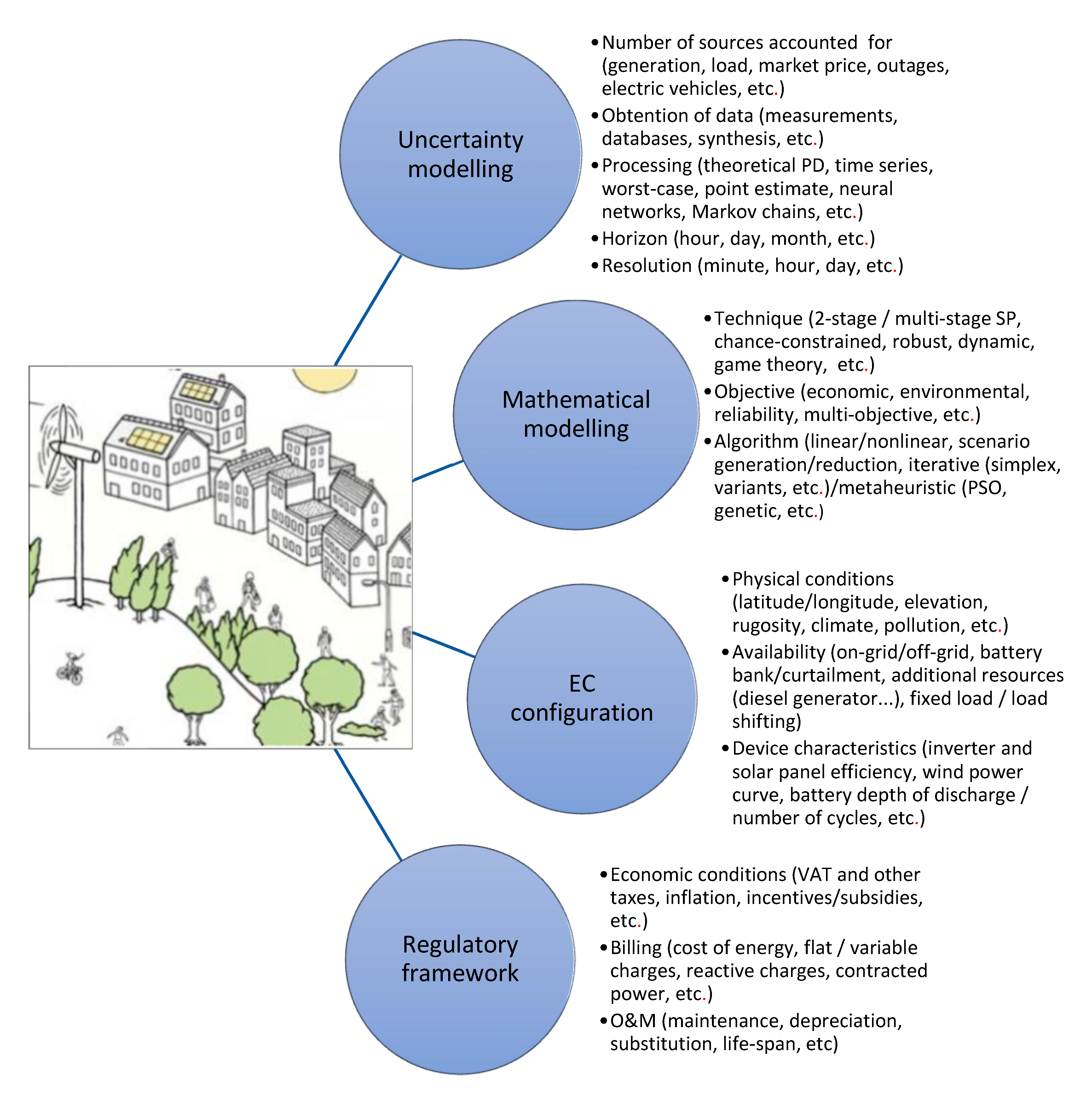
Figure 1.
Diagram of the microgrid model and its different subdivisions. Source: self-elaboration and River Cottage©.
Figure 1.
Diagram of the microgrid model and its different subdivisions. Source: self-elaboration and River Cottage©.
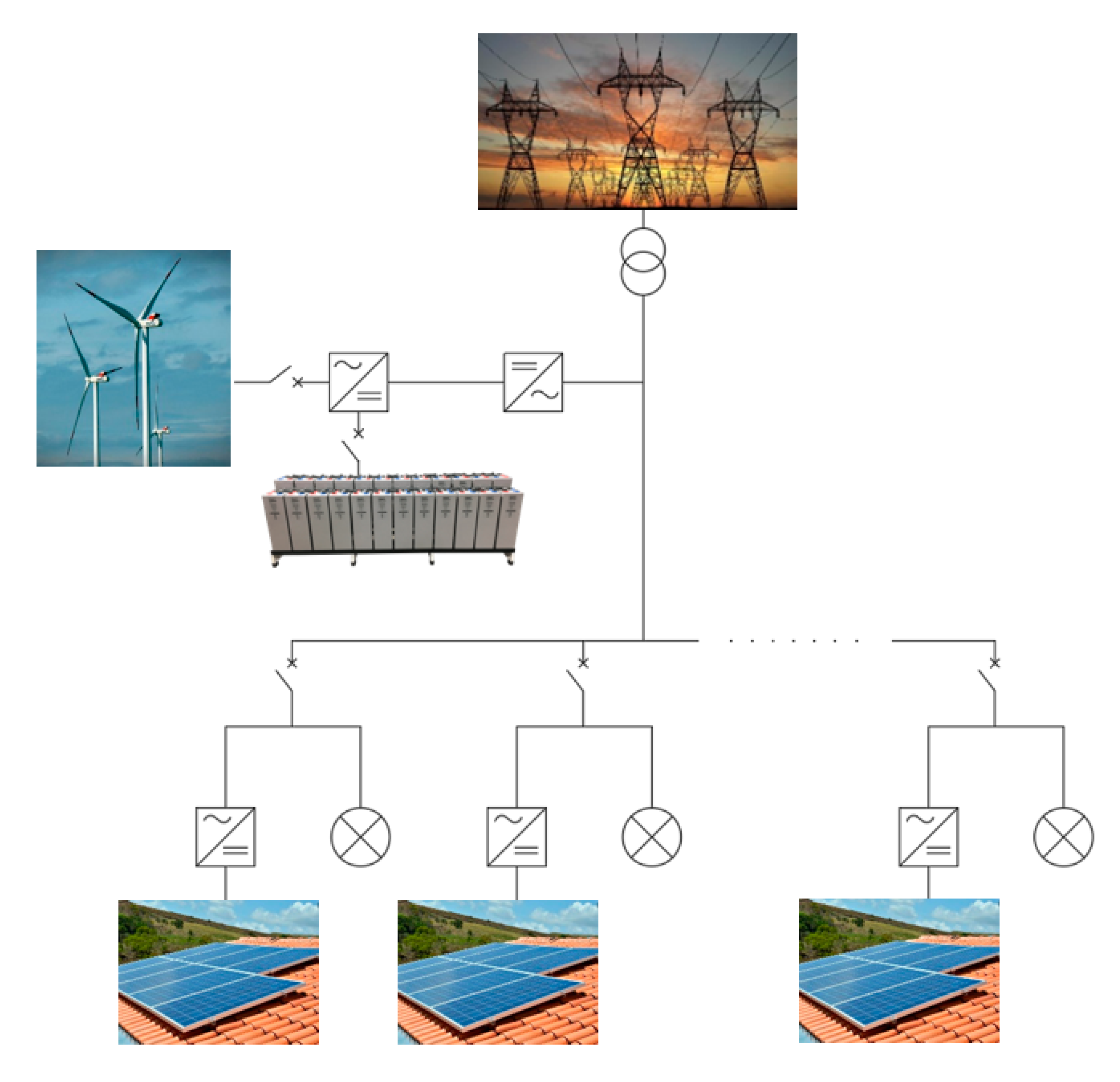
Figure 2.
Schematized representation of the microgrid configuration. Source: self-elaboration. Images under a CC BY-SA license.
Figure 2.
Schematized representation of the microgrid configuration. Source: self-elaboration. Images under a CC BY-SA license.
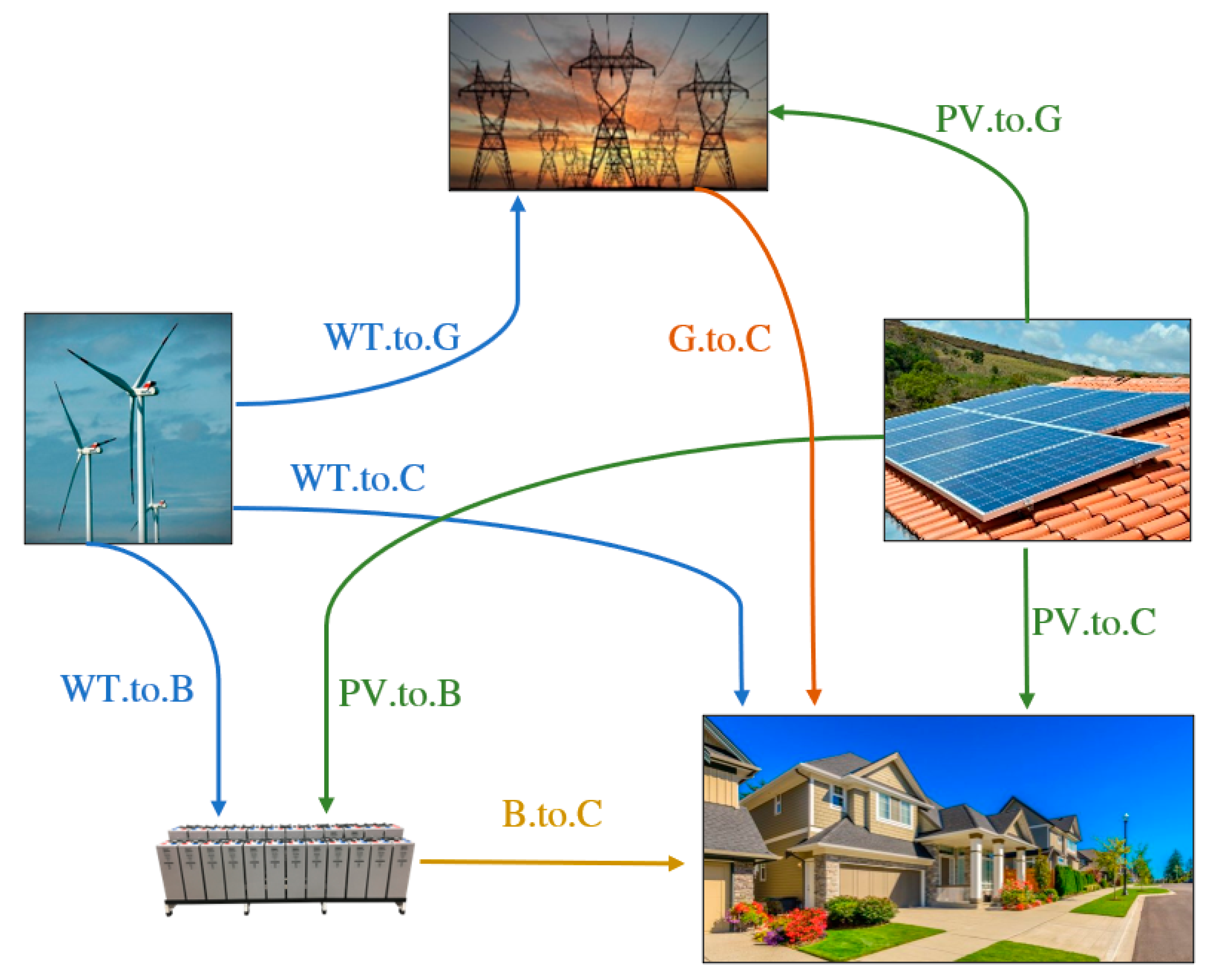
Figure 3.
Physical model and energy flows within the microgrid. Source: self-elaboration. Images under a CC BY-SA license.
Figure 3.
Physical model and energy flows within the microgrid. Source: self-elaboration. Images under a CC BY-SA license.
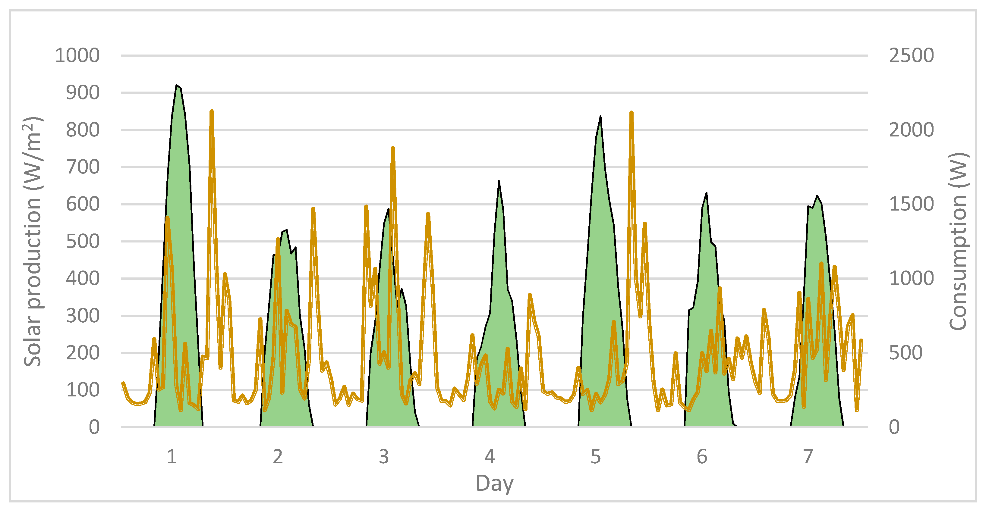
Figure 4.
Solar production (green) and individual consumption (orange) for the most probable scenario during one week of April. Source: self-elaboration.
Figure 4.
Solar production (green) and individual consumption (orange) for the most probable scenario during one week of April. Source: self-elaboration.
Figure 5.
Breakdown of the averaged annualized costs and earnings in the second stage for the energy community. Source: self-elaboration.
Figure 5.
Breakdown of the averaged annualized costs and earnings in the second stage for the energy community. Source: self-elaboration.
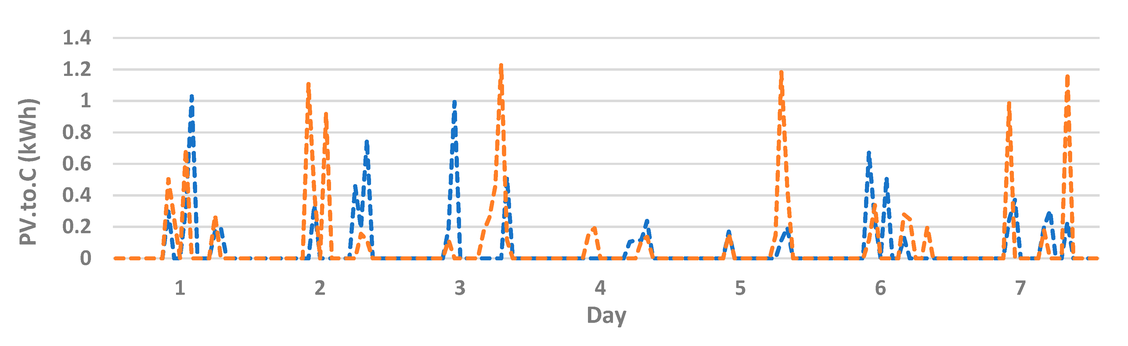
Figure 6.
Energy transmission from PV panels to loads for a single dwelling. Comparison between the most and least probable scenarios (blue and orange) for one week of April. Source: self-elaboration.
Figure 6.
Energy transmission from PV panels to loads for a single dwelling. Comparison between the most and least probable scenarios (blue and orange) for one week of April. Source: self-elaboration.
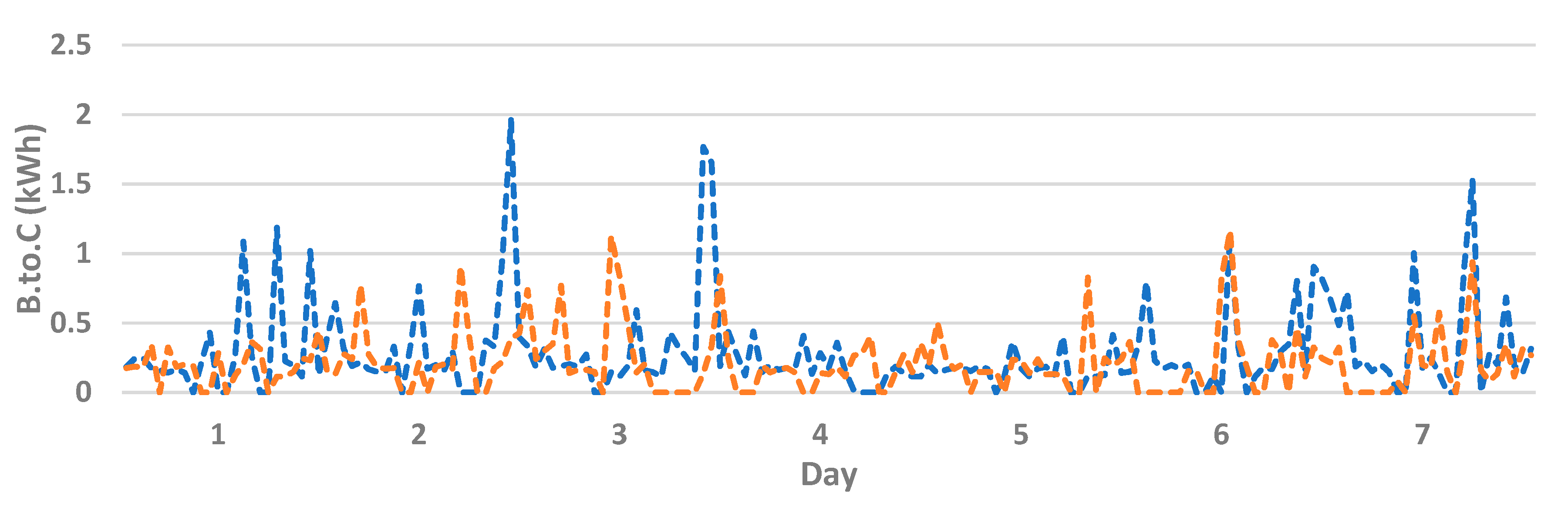
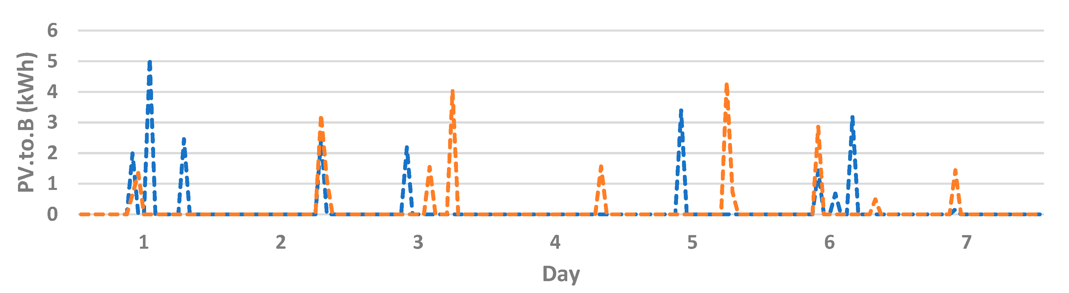
Figure 7.
Energy transmission from the battery bank to loads, for a single dwelling. Comparison between the most and least probable scenarios (blue and orange) for one week of April. Source: self-elaboration.
Figure 7.
Energy transmission from the battery bank to loads, for a single dwelling. Comparison between the most and least probable scenarios (blue and orange) for one week of April. Source: self-elaboration.
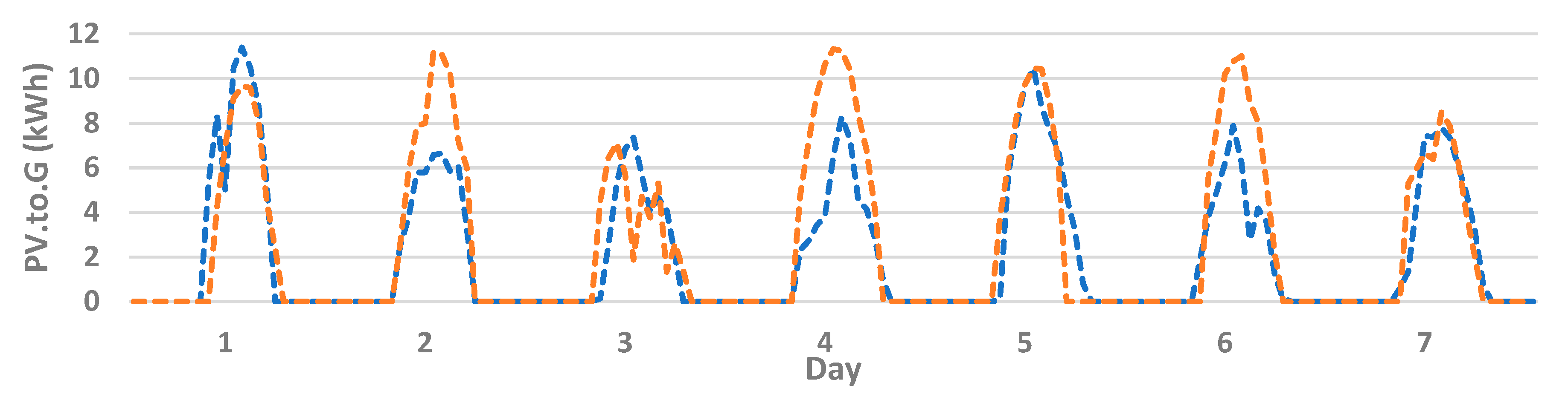
Figure 8.
Energy transmission from PV panels to the grid, for a single dwelling. Comparison between the most and least probable scenarios (blue and orange) for one week of April. Source: self-elaboration.
Figure 8.
Energy transmission from PV panels to the grid, for a single dwelling. Comparison between the most and least probable scenarios (blue and orange) for one week of April. Source: self-elaboration.
Figure 9.
Energy transmission from PV panels to the battery bank, for a single dwelling. Comparison between the most and least probable scenarios (blue and orange) for one week of April. Source: self-elaboration.
Figure 9.
Energy transmission from PV panels to the battery bank, for a single dwelling. Comparison between the most and least probable scenarios (blue and orange) for one week of April. Source: self-elaboration.
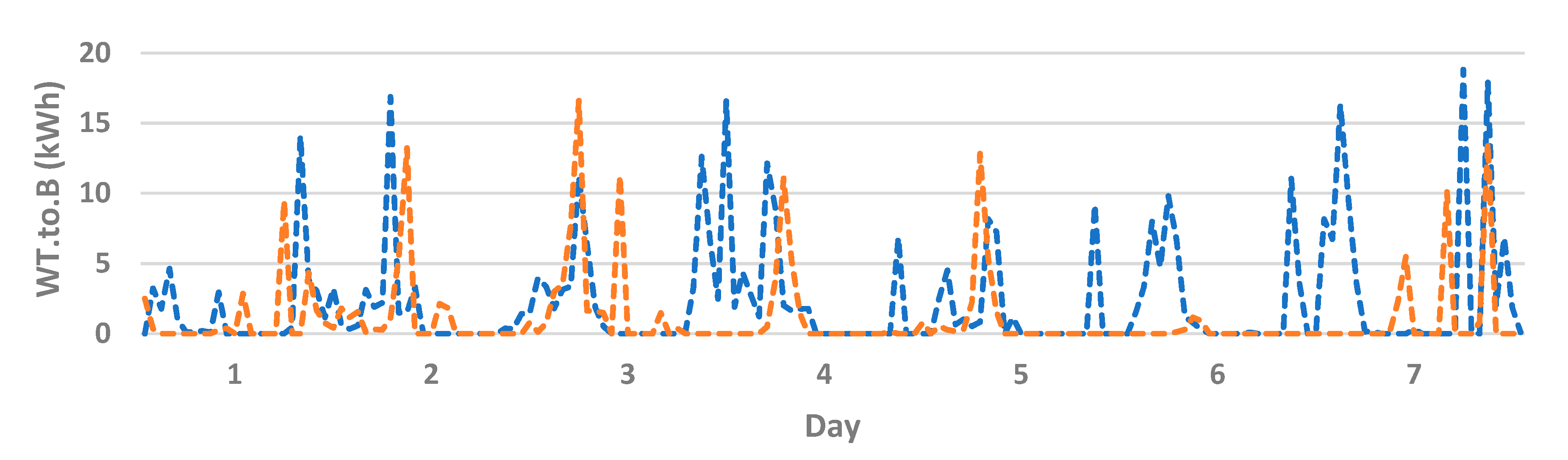
Figure 10.
Energy transmission from the wind turbines to the battery bank. Comparison between the most and least probable scenarios (blue and orange) for one week (April). Source: self-elaboration.
Figure 10.
Energy transmission from the wind turbines to the battery bank. Comparison between the most and least probable scenarios (blue and orange) for one week (April). Source: self-elaboration.
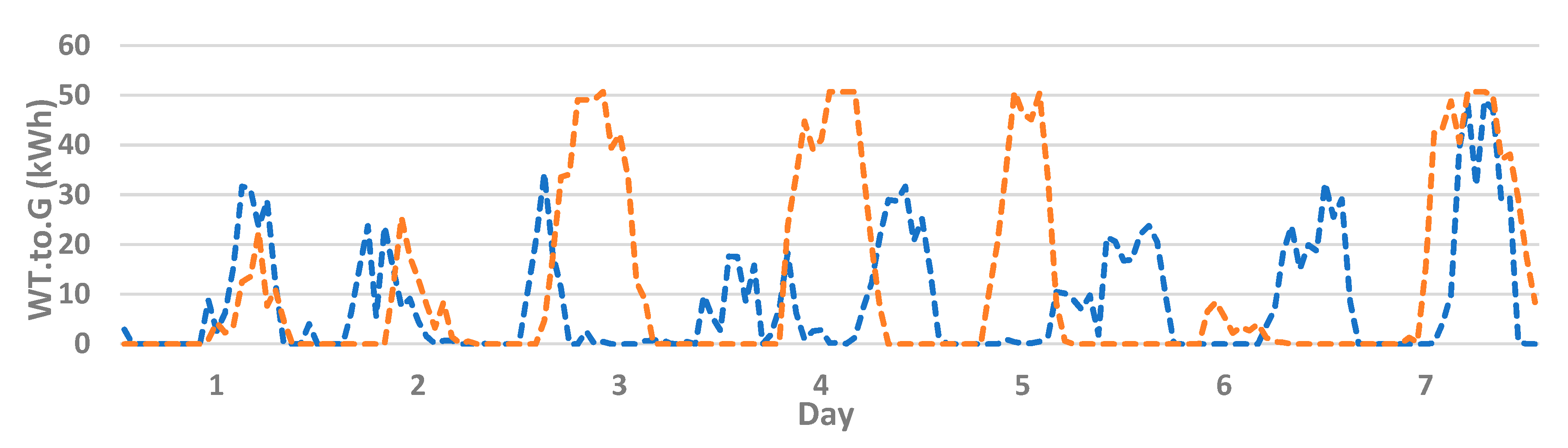
Figure 11.
Energy transmission from wind turbines to the grid. Comparison between the most and least probable scenarios (blue and orange) for one week of April. Source: self-elaboration.
Figure 11.
Energy transmission from wind turbines to the grid. Comparison between the most and least probable scenarios (blue and orange) for one week of April. Source: self-elaboration.
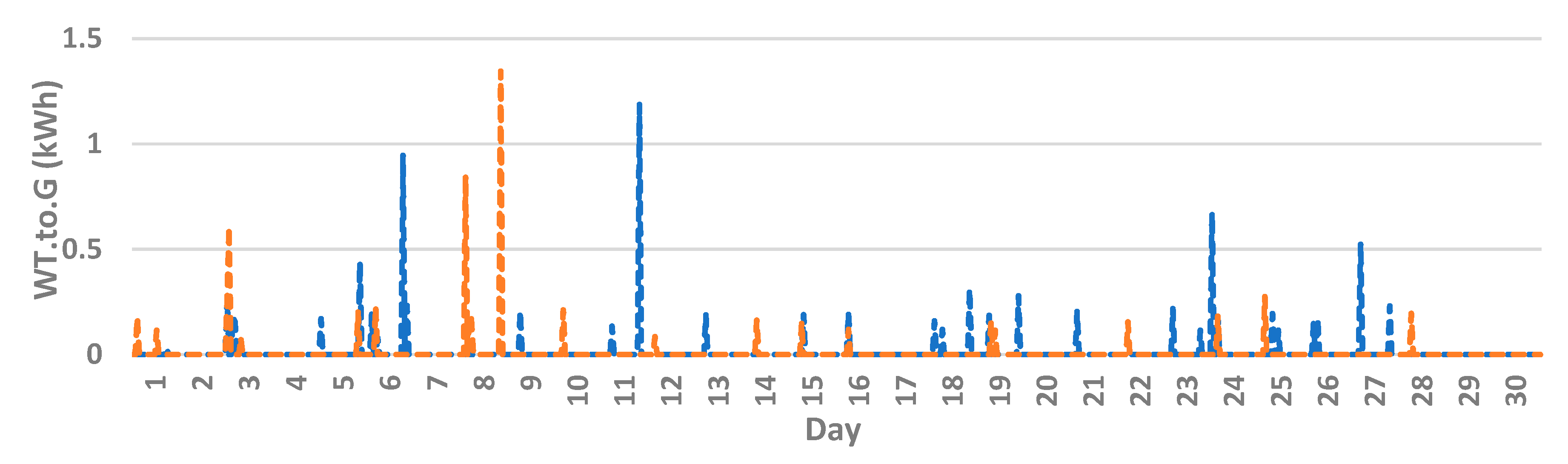
Figure 12.
Energy transmission from wind turbines to loads, for a single dwelling. Comparison between the most and least probable scenarios (blue and orange) for one month (April). Source: self-elaboration.
Figure 12.
Energy transmission from wind turbines to loads, for a single dwelling. Comparison between the most and least probable scenarios (blue and orange) for one month (April). Source: self-elaboration.
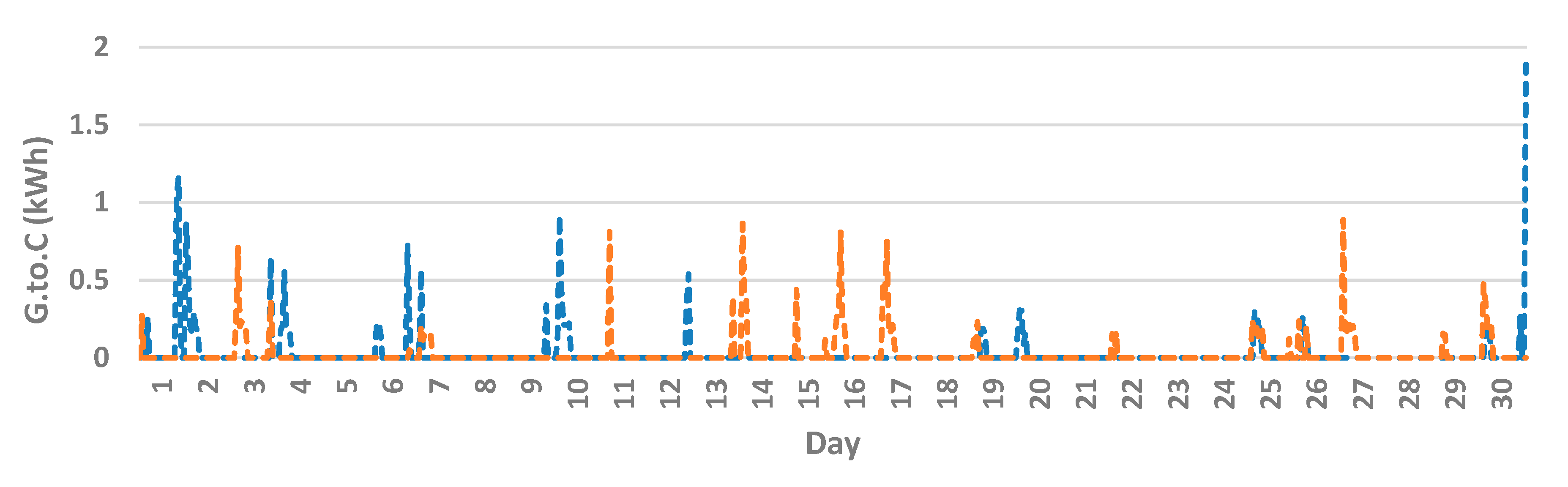
Figure 13.
Energy transmission from grid to loads, for a single dwelling. Comparison between the most and least probable scenarios (blue and orange) for one month (April). Source: self-elaboration.
Figure 13.
Energy transmission from grid to loads, for a single dwelling. Comparison between the most and least probable scenarios (blue and orange) for one month (April). Source: self-elaboration.
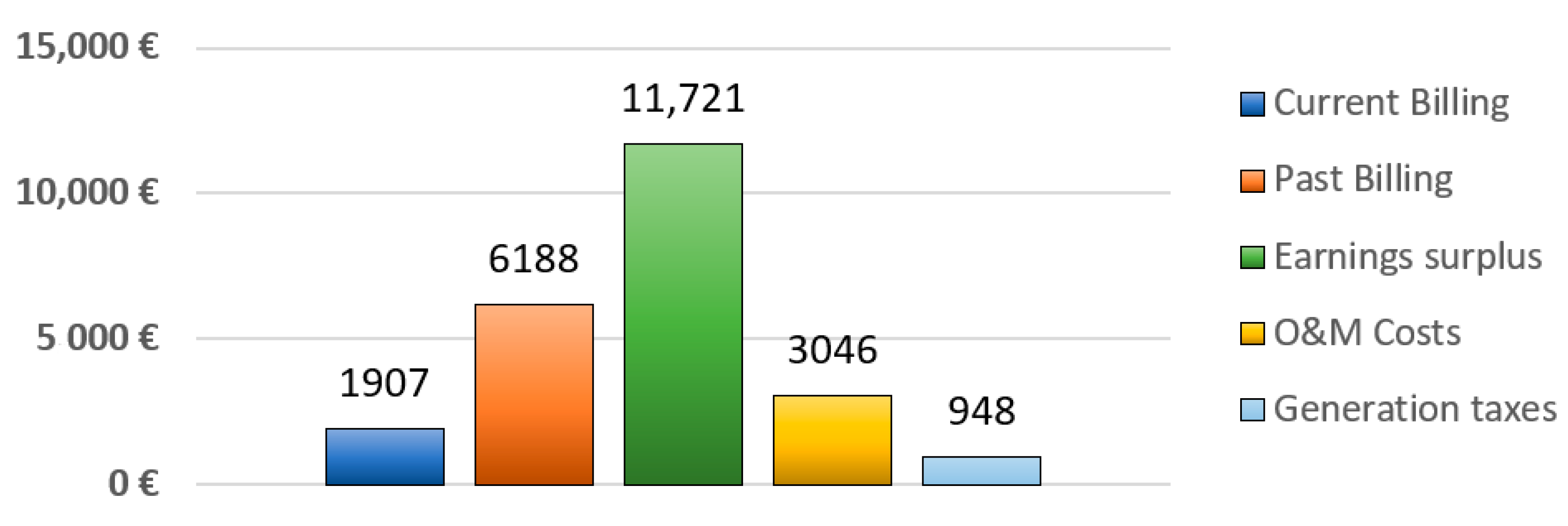
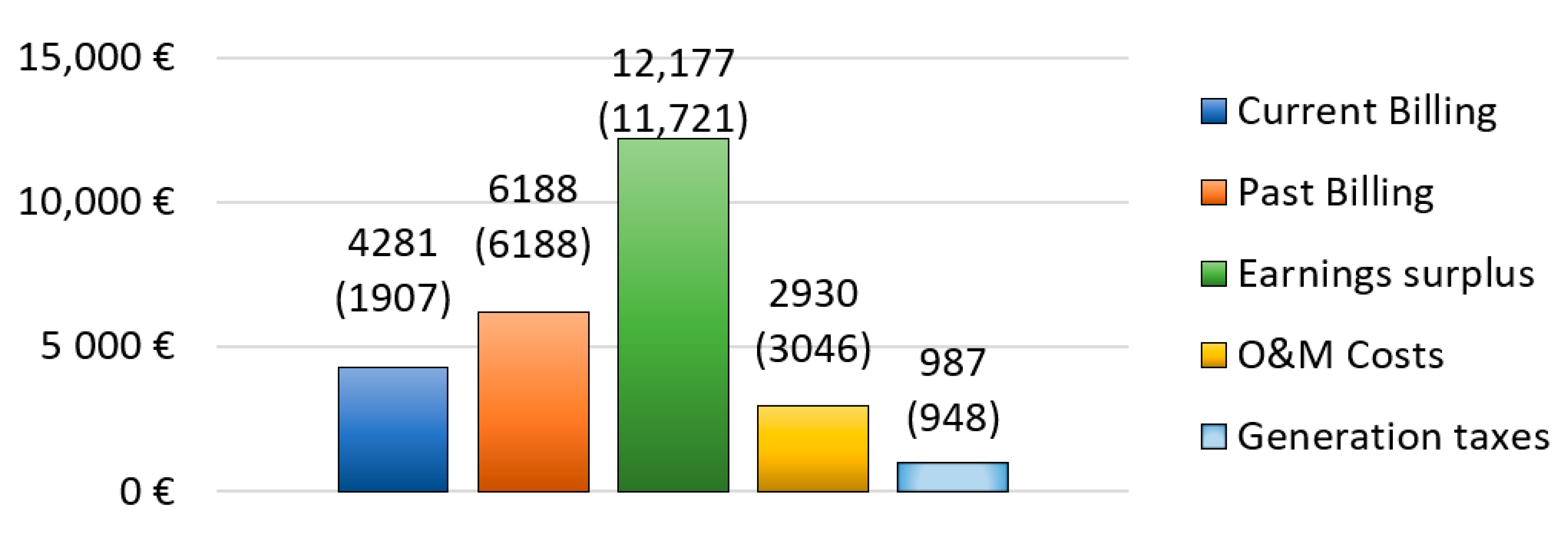
Figure 14.
Breakdown of the averaged annualized costs and earnings in the second stage for the energy community without energy storage. In parenthesis, the second stage costs for the model with energy storage. Source: self-elaboration.
Figure 14.
Breakdown of the averaged annualized costs and earnings in the second stage for the energy community without energy storage. In parenthesis, the second stage costs for the model with energy storage. Source: self-elaboration.
Figure 15.
Energy transmission from grid to loads in a system without energy storage, for a single dwelling. Comparison between the most and least probable scenarios (blue and orange) for one month (April). Source: self-elaboration.
Figure 15.
Energy transmission from grid to loads in a system without energy storage, for a single dwelling. Comparison between the most and least probable scenarios (blue and orange) for one month (April). Source: self-elaboration.
Table 1.
Sets of the mathematical program.
Table 1.
Sets of the mathematical program.
|
Set
|
Index
|
Definition
|
Elements
|
|---|
| Hours | h | Set of hours of the year | 1 .. T |
| Dwellings | d | Set of dwellings of the energy community | 1 .. D |
| Scenarios | s | Set of scenarios of the second stage variables | 1 .. S |
Table 2.
Parameters related to renewable generation.
Table 2.
Parameters related to renewable generation.
|
Parameter
|
Definition
|
Value
|
|---|
| RPS | Ratio between peak power and surface of the panel | 180 W/m2 |
| Smaxd | Maximum surface that can be occupied by solar panels | 0–50 m2 |
| Maximum PV potential on each hour | 0–10 kWh |
| Maximum wind power potential on each hour | 0–50 kWh |
| P_WTmax | Nominal power of wind turbines | 10 kW |
| N_WTmax | Maximum number of wind turbines to install | D/2 |
| panels | Mean efficiency of the solar panels | 18% |
| inverter | Simplified constant efficiency of the inverter | 98% |
| Maximum power admission of the low voltage three phase lines | 50 kW |
Table 3.
Parameters related to energy storage.
Table 3.
Parameters related to energy storage.
|
Parameter
|
Definition
|
Value
|
|---|
| B_max | Maximum capacity of the battery bank | D * 9 kWh |
| bat | Charging/discharging efficiency of the batteries | 99% |
| SoC_min, SoC_max | Minimum and maximum State of Charge | 20%, 100% |
| SoC_0 | Initial SoC of the batteries | 20% |
| PBat_max | Maximum charge/discharge power of the battery bank | B max/1h (kW) |
Table 4.
Parameters related to the sources of uncertainty or stochastic parameters of the physical constraints.
Table 4.
Parameters related to the sources of uncertainty or stochastic parameters of the physical constraints.
|
Parameter
|
Definition
|
Value
|
|---|
| Probs | Probability of scenario s | 0–1 |
| Cd,h,s | Electrical consumption | 0–3 kWh |
| Ih,s | Solar irradiance | 0–1000 W/m2 |
| PWTh,s | Wind turbine supplied power | 0–10 kW |
Table 5.
Variables related to physical constraints.
Table 5.
Variables related to physical constraints.
|
Variable
|
Definition
|
|---|
| EGPVd,h,s | Generated PV energy (kWh) |
| Energy flow from solar panels to consumption |
| Energy flow from solar panels to the grid |
| Energy flow from solar panels to the battery bank |
| Sd | Area occupied by solar panels for each dwelling |
| EGWTh,s | Generated WT energy (kWh) |
| Energy flow from wind turbines to grid |
| Energy flow from wind turbines to the battery bank |
| Energy flow from wind turbines to consumption |
| Number of wind turbines to install |
| Bh,s | Stored energy (kWh) |
| BCap | Capacity of the battery bank |
| Energy flow from the battery bank to consumption |
| Energy flow from the grid to consumption |
| EB_Ch,s | Battery charging energy (kWh) |
| EB_Dh,s | Battery discharging energy (kWh) |
| Peak PV power to install in each dwelling (kW) |
Table 6.
Parameters related to energy costs.
Table 6.
Parameters related to energy costs.
|
Parameter
|
Definition
|
Value
|
|---|
| COpmPV | O&M cost of PV power [16] | 16 €/kWp·year |
| COpmWT | O&M costs of onshore wind power [16] | 26.6 €/kWp·year |
| COpmBat | O&M costs of lithium-ion batteries [17] | 6.1 €/kWh·year |
Table 7.
Parameters related to the energy sale.
Table 7.
Parameters related to the energy sale.
|
Parameter
|
Definition
|
Value
|
|---|
| SellingPriceh,s | Selling marginal price of surplus electricity | MarketPriceh,s |
| FTax | Flat tax over sold energy | 7% |
| VTax | Variable tax over sold energy | 0.5 c€/kWh |
Table 8.
Parameters related to the energy billing.
Table 8.
Parameters related to the energy billing.
|
Parameter
|
Definition
|
Value
|
|---|
| Pcond | Contracted power without self-consumption | 2.3–9.2 kW |
| VAT | Value Added Tax | 21% |
| ETax | Flat tax over purchased electricity | 5.11% |
| Variable charges over purchased electricity [16] | 0.044027 €/kWh |
| Tp | Flat charges over purchased electricity [16] | 38.04 €/kWh·year |
Table 9.
Parameters related to the sources of uncertainty or stochastic parameters of the economic constraints.
Table 9.
Parameters related to the sources of uncertainty or stochastic parameters of the economic constraints.
|
Parameter
|
Definition
|
Value
|
|---|
| MarketPriceh,s | Purchase price of energy at the electricity market | 0–180 €/MWh |
Table 10.
Variables related to economic constraints.
Table 10.
Variables related to economic constraints.
|
Variable
|
Definition
|
|---|
| New contracted power after the installation of the community microgrid (kW) |
| CEd,s | Cost of energy purchase (€) |
| PAd,s | Access Cost of energy purchase (€) |
| FSEd,s | Total cost of energy purchase (€) |
| TAXd,s | Total cost of taxes for selling energy (€) |
| INGd,s | Revenue for the sale of energy (€) |
| COpmd,s | Total O&M costs (€) |
Table 11.
Parameters related to investment cost.
Table 11.
Parameters related to investment cost.
|
Parameter
|
Definition
|
Value
|
|---|
| CInvPV | Investment cost of PV power [16] | 1150 €/kWp |
| CInvWT | Investment cost of onshore wind power [16] | 1700 €/kWp |
| CInvBat | Investment cost of lithium-ion batteries [17] | 795 €/kWh |
Table 12.
Parameters of the simulation.
Table 12.
Parameters of the simulation.
|
Set
|
Parameter
|
Value
|
|---|
| Hours | T | 8760 |
| Dwellings | D | 10 |
| Scenarios | S | 10 |
| 0.25 | 0.20 | 0.14 | 0.11 | 0.08 | 0.07 | 0.06 | 0.04 | 0.03 | 0.02 |
Table 13.
Results of the on-grid model: First-stage variables and objective function.
Table 13.
Results of the on-grid model: First-stage variables and objective function.
|
Variables
|
Value
|
|---|
| 10 kWp/dwelling (upper limit) |
| N_WT | 5 (upper limit) |
| BCap | 19.0 kWh |
| CInv | 230,210 € |
| Pcon’d | 2.64 kW/dwelling |
| Objective function z | −2799 €/year |
Table 14.
Results of the on-grid model with no storage: First-stage variables and objective function.
Table 14.
Results of the on-grid model with no storage: First-stage variables and objective function.
|
Variables
|
Value
|
Difference with the Base Case
|
|---|
| 10 kWp/dwelling (upper limit) | No difference |
| N_WT | 5 (upper limit) | No difference |
| BCap | 0 kWh | −19.0 kWh |
| CInv | 200,000 € | −30,210 € |
| Pcon’d | 4.6 kW/dwelling | +1.96 kW/dwelling |
| Objective function znb | −2167 €/year | +632 €/year |
Table 15.
Quality metrics definition and value.
Table 15.
Quality metrics definition and value.
|
Variable
|
Definition
|
Value
|
|---|
| z | Original objective function | −2799 €/year |
| Objective function fixing the first stage variables to the solution that would be employed intuitively, without an optimization approach | −360 €/year |
| Objective function fixing the first stage variables to the results obtained in the expected value program. | −2371 €/year |
| PO | Performance of Optimization metric | 2439 €/year |
| VSS | Value of Stochastic Solution metric | 428 €/year |

 ,
, 


