A Logistics Management System for a Biomass-to-Energy Production Plant Storage Park

Abstract

The biomass industry is growing due to the current search for greener and more sustainable alternatives to fossil energy sources. However, this industry, due to its singularity, presents several challenges and disadvantages related to the transportation of raw materials, with the large volumes that are usually involved. This project aimed to address this internal logistics situation in torrefied biomass pellets production with two different biomass storage parks, located in Portugal. The main park receives raw material coming directly from the source and stores it in large amounts as a backup and strategic storage park. The second park, with smaller dimensions, precedes the production unit and must be stocked daily. Therefore, a fleet of transport units with self-unloading cranes is required to help to unload the biomass at the main park and transport the raw material from this park to the one preceding the production unit. Thus, the main goal was to determine the dimensions of the fleet used in internal transportation operations to minimize the idle time of the transport units using a methodology already in use in the mining and quarrying industry. This methodology was analyzed and adapted to the situation presented here. The implementation of this study allows the elimination of unnecessary costs in an industry where the profit margins are low.

1. Introduction

Energy resources play a crucial role in the shifting dynamics of the global energy scenario [1]. Energy is considered one of the primary agents of wealth generation and economic development [2]. Currently, global warming and the reduction in oil reserves are challenges of extreme relevance that have encouraged the search for alternative energy sources [3]. Thus, the use of renewable forms of energy is a pressing goal for all governments in order to comply with international treaties designed to impose targets for the reduction in greenhouse gases as a measure to mitigate climate change [4]. In this framework, there are energy systems supported by widely adopted renewable energy sources, such as hydropower, wind, and solar [5]. However, these energy sources are dependent on the seasonality of the resources used to produce energy and are dependent on the intermittency caused by the dependence on the weather conditions [6]. This implies that these systems require support and backup systems that can inject energy into the power grid whenever the energy produced is not enough [7].

Biomass is a good alternative to the above-mentioned energy sources, as it is renewable and widely available and also has the possibility to be stored and used immediately when needed [8]. Biopower also promotes the elimination of residual and waste biomass forms from, for example, forestry operations, agriculture, and industry, thereby reducing the risk of rural fires and volume reduction when landfill is the chosen option [9]. Among others, the main advantages of biomass include the flexibility, wide availability, and carbon neutrality [10]. This latter so-called advantage is based on the principle that all sources of biomass when burnt release the same amount of carbon dioxide stored during the lifetime of the plants [11].

Biomass do not offer the best characteristics as fuel, mainly due to the low density, low heating value, heterogeneity, geographic dispersion, high storage volumes, and high moisture typically presented [12,13]. These factors imply that, in the majority of the situations, it is very difficult to achieve productivity rates that allow for optimization of the logistics associated with biomass [10,14]. Currently in industry, various forms of solid biomass are widely used, with a special emphasis on wood chips and a recent focus on biomass pellets [15]. Pellet production has increased significantly in recent years [16]. After a slight increase in 2016, production increased by 11% the following year [17]. The origin of this increase was the high demand that has been verified for this product, particularly in Europe, which currently has the largest consumption of pellets in the world [18]. Regarding the purpose for which they are used, 55% is for domestic use and 45% for industrial applications [19]. In Europe, the use of pellets has increased both domestically and industrially; however, industry accounts for the majority of this increase [20]. In Portugal, the market consists of small direct consumers with small and medium consumption peaks in the winter period, from October to April [21]. The main consumer sectors of biomass pellets in Portugal are the domestic sector, public services, and small industries with specific thermal energy needs [22]. Included here are the heating systems in large service buildings, such as schools, hospitals, nursing homes, swimming pools, and other similar structures [21].

More recently, a new group of consumers emerged that, due to their large thermal energy needs, began to look for cheaper forms of energy [23]. This group includes textile dyeing units, which are important for the Portuguese economy [24]. There is also the potential to extend the consumption of pellets to other industries in the country; the fact that there are areas of Portugal with high amounts of biomass residues coming from forestry activities or agricultural activities makes this source of energy viable in comparison to fossil fuels [22,25]. The consumption of pellets at the domestic level is an area that has great potential due to the advantages they offer, which threatens to overtake other types of energy sources [26]. Among others, the most relevant advantages are reduced heating costs, the possibility of buying small quantities of pellets, better management of the family budget, technological versatility, and low carbon dioxide emissions, which is increasingly a concern of the general population and leads consumers to seek clean energy [27].

The methodology used in this study is based on the transposition of knowledge already in use in other disciplines. In this particular case, this methodology was developed for use in the mining and quarrying industry, and primarily developed and presented by authors from the Department of Mining Engineering of the Faculty of Engineering of the University of Oporto (Portugal) who studied these fields of engineering. Relevant studies include those presented by Botelho de Miranda (1986), Leite (1990), Leite (1994), Botelho de Miranda and Leite (1996), and the final compilation of information presented by Botelho de Miranda (2005), which is now adapted to the biomass sector [28,29,30,31,32].

Despite the fact that these procedures have long been used in other sectors of industrial activity, namely, in the mining and quarrying industry, the novelty of this approach is precisely the importation of these methods and techniques to the biomass industry sector. In spite of the differences between the scenarios, the processes and the procedures used present many similarities. For example, in quarrying operations the raw material is transported from the dismantling front to the storage park that feeds the primary crusher, while in a biomass pellet production unit, the raw material arrives from the forest, is unloaded in a park that ensures the permanent availability of raw material, which can be compared, in the quarrying industry model, to the quarry, and the shredder of the biomass pellet plant, to the primary crusher. This study applies to an example of relatively small dimensions. However, the purpose is to create a launching base for large biomass storage parks, which can be found, for example, in the pulp and paper industry, or in those larger biomass conversion units that are expected to start emerging in the near future, to present reliable solutions for coal replacement in thermal power plants.

The objective of this study, which can be considered a case study, is the development of a logistics management system for a biomass storage park, in this situation associated with a large torrefied biomass production unit, and that was based on a methodology already well-known and implemented in the quarrying and mining industry. That is, a solution that minimizes permanent and strategic stocks, optimizes the production line supply routes, and reduces the dead time of the equipment. With these objectives in mind, the main focus of this study was the dimensioning of the truck fleet, which, in the first instance, will unload the external trucks (ETs) that arrive at the larger capacity biomass storage park (P1) loaded with biomass, and that do not have the means to unload without aid. Once this function is complete, when no more trucks need to be unloaded, the same fleet will transport biomass from P1 to the smaller capacity biomass storage park (P2). This ensures that all external trucks transporting biomass to P1 are unloaded and that the amount of daily biomass required by the production unit is then transported to P2. To this end, issues, such as the routes to be used by the truck fleet to transport biomass from P1 to P2, the cycle times of the operation, the efficiency of the trucks, and the available infrastructure, must be well analyzed in order to construct a robust and feasible solution, and that launches the basis for the replication of the model in other biomass industry projects in the future.

2. Materials and Methods

2.1. Case Study Framework

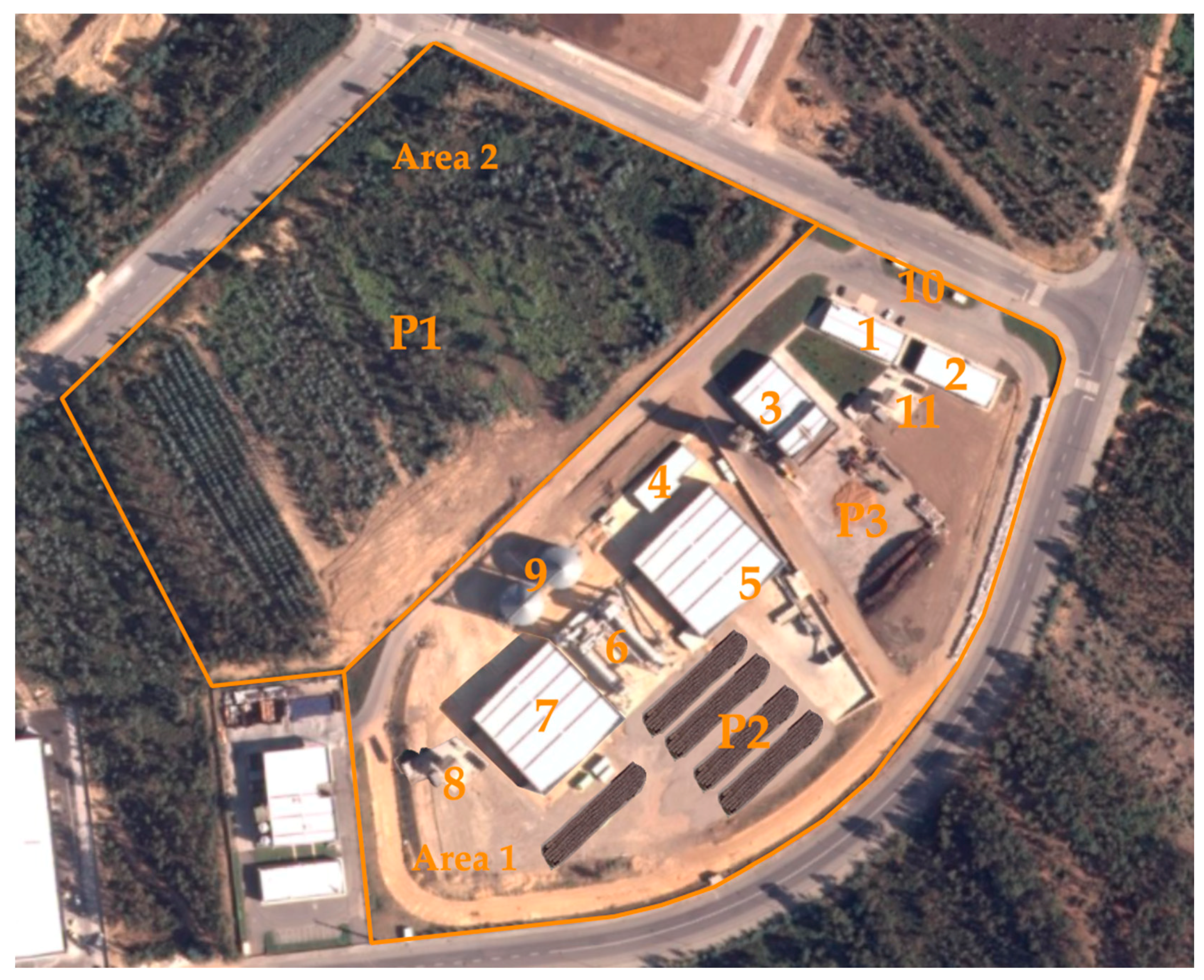
This case study was performed and implemented at Advanced Fuel Solutions SA (AFS), a company located in Oliveira de Azeméis (North Portugal). AFS is a company focused on the research and production of fuels with high added value, based on the conversion of biomass using torrefaction. The company has two production units located on the same industrial platform, one that is smaller and more dedicated to research and development, with an annual production capacity of 3000 tons and an industrial size unit, with a production capacity of torrefied biomass pellets of 96,000 tons/year. Figure 1 shows the different units and sections deployed in the same location.

The AFS production process, as previously mentioned, aims to continuously produce pellets and torrefied biomass. We can divide the organic units as follows:

• Raw material storage park: The raw material warehouse consists of the storage facilities P1 and P2, with the ordinance, which includes the weighbridge for weighing trucks as a support tool. Park P2 is intended for the storage of direct support to production, having permanently a stock equivalent to the daily consumption of production. In other words, this park should have a quantity of wood corresponding to 24 h of production, divided into three 8-h shifts, starting at 00:00 a.m., totaling approximately 900 tons of stock, which will correspond to a production of approximately 288 tons of pellets of daily torrefied biomass. Park P1 is intended to store a stock of raw material corresponding to 3 months of production, in order to serve as a buffer to any eventuality that may force the stop of the production unit for reasons beyond its management, such as bad weather that prevents the delivery of raw materials by suppliers, strikes, or others, which is why it is considered the strategic reserve of raw materials.
• Raw material pre-processing section: After receiving the raw material and storing it in a park, the next step is to go into production. Preferably, the raw material is received in the form of logs, also called roundwood, which enters the production process through the first operation, which is dehulling. In this equipment, called a peeler, the bark is removed from the trunks, which proceed to the next stage, the destruction. The removed peel goes in the opposite direction, being a valuable by-product. The trunks then advance to shredding, passing through a conveyor belt where the inert cargo that may still accompany the raw material is removed, then, passing through a metal detector, thus, preventing metal parts from entering the shredder, damaging the blades. This operation is important, as the good operation of the shredder depends on the state in which the blades are in, and contact with metal parts decreases their useful life, anticipating stoppage for their replacement. The shredder will reduce the logs to pieces with a variable size, usually G30, so then the material goes through a conveyor belt to a screen, where it will be selected according to the desired size. All material that is not yet as intended, returns to the shredder, while the material that is already in compliance, goes to intermediate storage. This intermediate storage consists of a pile placed on a mobile floor driven by a hydraulic system, which transfers the chip to a system of conveyor belts, which in turn will feed the biomass dryer, which is detailed in the next section.
• Biomass drying and torrefaction section: The drying unit consists of a single pass rotary drum dryer, where the chips, theoretically with a humidity close to 50%, will dry until reaching a humidity close to 20% to 22%, and is then passed to the torrefaction reactor. This reactor, also of the rotating drum type, operates at a temperature between 220 and 320 °C, depending on the type of biomass to be processed and the degree of torrefaction that is to be reached. During the process the released torrefaction gases are recovered and used as an energy source. After the torrefaction phase, the material advances to the cooling system, which is composed of a series of double-wall endless conveyors with counter-current water circulation, which is cooled by a cooling system placed outside. After this process, the material goes to the densification section.
• Densification section: After having cooled, the material can finally start the densification process, which, in this specific case, is conducted using horizontal axis ring matrix pelletizers. For this, the material will be milled, using a millstone, and immediately transferred to an intermediate storage silo, which ensures the constant supply of the pelletizing system, consisting of a series of pieces of equipment, with a pelletizing capacity of 12 tons/hour. After pelletizing, the finished product will cool using an air-to-current cooler and proceed to the finished product silos.
• Finished product storage and shipping: This system consists of two silos with a capacity of 2500 tons each, with a direct truck loading system, for single and exclusively bulk shipping.

The production unit of the company has two biomass storage parks, the main one with larger capacity (P1), which will receive the biomass directly from the external suppliers, and another one, with smaller size (P2), which precedes the production line and is supplied from P1. P1, due to its larger dimensions, allows the biomass storage in the longer term and is supplied daily by external trucks (ETs). Of these trucks, only a few have cranes that allow them to unload themselves, which implies that the others must be unloaded, forcing the presence of a machine in the park capable of performing this task.

P2, in addition to the strategic stock in P1, will store the amount of biomass that the production unit processes daily. Thus, biomass must be transported every day from P1 to P2 to satisfy the needs of the production unit. Based on the above, the company must have equipment to unload the trucks without cranes at P1 and to transport biomass from P1 to P2. A truck or fleet of trucks is needed for this transport, and, as far as the unloading task at P1 is concerned, one or more cranes are necessary. Since the supplying of P1 is done at a specific daily interval, this implies that the cranes would only be useful in this interval and would be inactive for the rest of the day. Therefore, the solution studied consists of the use of a truck or a fleet of trucks equipped with cranes, which perform either the unloading operations at P1 or the transport to P2.

2.2. Raw Materials Logistics Configuration and Description

2.2.1. Internal Transport System

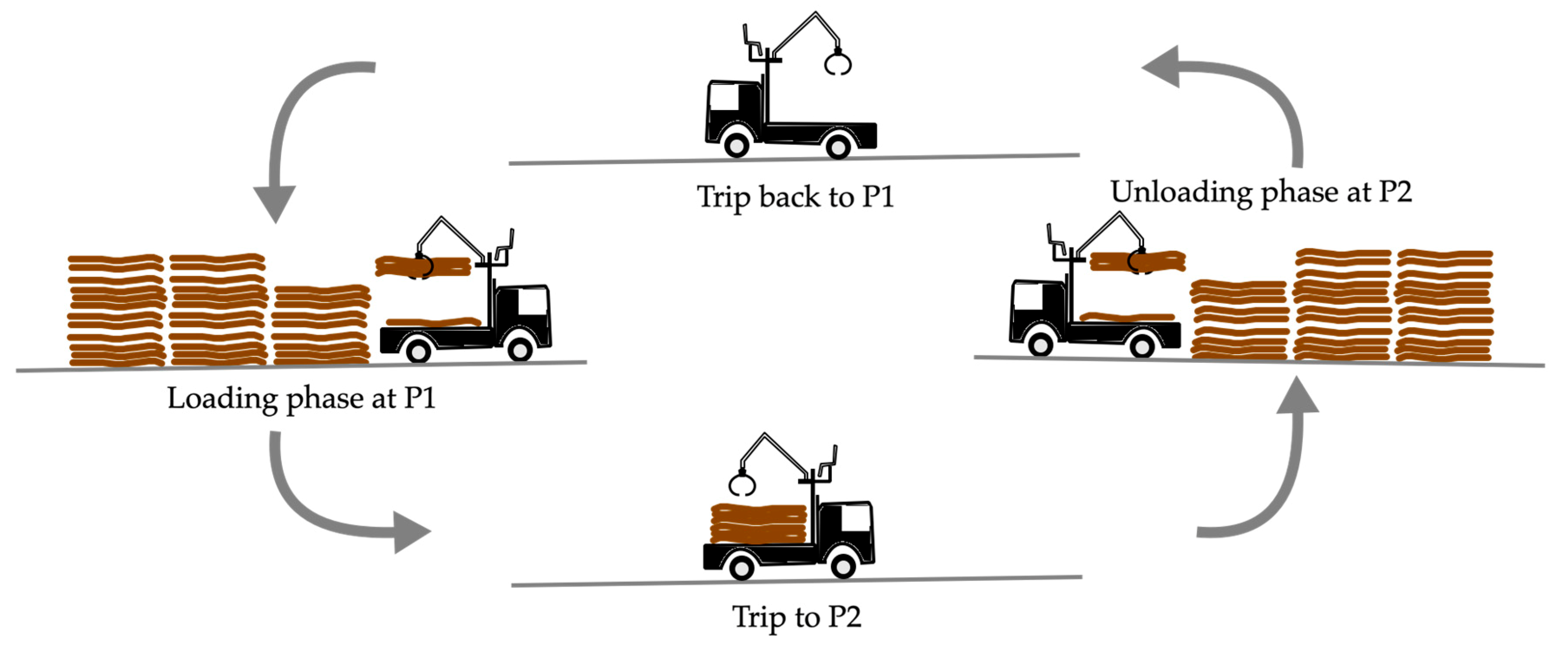
The role of the raw material transport systems is essentially to transfer materials from a given location to another one, which can be various distances away, and can be deposited and stored or temporarily stored before processing. The fleet to be dimensioned consists of loading units (LUs) and transport units (TUs). In this case study, the situation is similar, as it is the transport of materials stored in a biomass park to a smaller park that precedes the production line, where it will be processed. The material coming from the park intermittently comes to the place where it is deposited using TUs, which, in terms of performance, may or may not constitute a homogeneous set. The TUs are equipped with cranes that allow the loading and unloading steps to be carried out without the aid of LUs.

Each TU performs a cyclic task composed of four phases (Figure 2):

• the loading phase at P1;
• the trip to the production unit;
• the unloading phase at P2;
• the trip back to P1.

The material to be transferred is stored at P1 through an external supply carried out periodically throughout the day, which ensures that the TUs will not create a queue at the place of loading due to a lack of raw material. The same can be said in relation to the unloading site, as the park where the biomass will be unloaded always has sufficient space for storage. Another difference between the situation under study and the one in the analyzed bibliographic references is that the TUs, in addition to transport, are in charge of unloading the ETs arriving at P1 with biomass. Once the phases and elements of the system have been defined, it is necessary to study the time spent in the activities, as these are not constant and vary according to several factors that will be identified.

2.2.2. Transportation Units Synchronism

One of the aspects receiving the most focus in the literature under study is the use of synchronism as a criterion for sizing the fleet. Synchronism is based on the principle that LUs will never be inactive due to the lack of TUs to be loaded and that TUs never have to wait for the opportunity to be served by LUs. As already mentioned, in this project, the fleet consists only of one type of unit, trucks with cranes, which are represented by TUs. These TUs are able to perform the tasks of loading and unloading autonomously; however, the notion of synchronism can also be applied in this context. In this system, it may be considered that the synchronism criterion is based on the assumption that the time required for TUs to perform their work coincides with the time of each shift. In other words, it should be ensured that TUs are not stopped because there are no tasks to be performed, and, on the other hand, that there are no remaining tasks because there is not enough time to complete them during the shift. In real systems, synchronism will never be achieved permanently. The variability of activity times and the fact that the number of TUs is necessarily an integer will ensure that synchronism cannot be achieved consistently.

2.2.3. Algorithm Configuration

Adopting average values to represent the times of productive and non-productive activities of the equipment is a simplified approach that is used for the sizing of fleets. However, this approach does not translate reality into study, as the times vary around the means, and this variability often follows statistical regularities that allow the use of known probability laws. Invoking these laws provides the structuring of stochastic simulation algorithms for transport systems. These algorithms produce results that are more rigorous than those derived from deterministic algorithms, in addition to providing multifaceted, subtle, and detailed information regarding the system performance. The variability is due to stops and/or variations in the productivity of the equipment, which can lead to gains or losses of time around the mean. However, temporal variations determine the average systematic efficiencies of the ideal efficiency of 100%.

As to the origin of the lost time or stretches of time for executing productive activities, there can be physical or non-physical causes originating from the following factors, as described by Botelho de Miranda (1986), Leite (1990), Leite (1994), Botelho de Miranda and Leite (1996), and Botelho de Miranda (2005) [28,29,30,31,32]:

• Nature and conditions of the material to be moved, namely the blocometry and degree of humidity.
• Poor conditions of the track and peculiarities of its layout.
• Insufficient space for TU positioning maneuvers in the loading and unloading phases.
• Incorrect positioning of TUs in relation to the material to be loaded or the place of unloading.
• Spontaneous climatic instability.
• Poor mechanical condition of the equipment.
• Insufficient capacity of the storage park.
• Dimensions and types of equipment and their maneuverability.
• Functional or design features of the mobile equipment.
• Stability of the operating regime of the production unit.
• Interference between the various mobile and/or fixed entities that are part of the system, which may result in queues for loading and unloading.
• Psychological posture of operators in the face of adverse climatic conditions or potentially dangerous handling circumstances.
• Malpractice, poor training, and/or lack of professional awareness of equipment operators.
• Immobilization of equipment for light maintenance/checking routines resulting from quick repairs or for refueling.
• Sporadic immobilization to receive directives/instructions from supervisors or to transmit diverse information.
• Incorrect supervision of services.
• Long-term immobilization for specific reorganization of the operating schemes.
• General reorganization of services.
• Night work.
• Unpredictable (serious damage or accidents) or programmed (deep maintenance/review actions) equipment immobilization.
• General weather conditions combined with climatic seasonality.
• Stretching of activity times by traffic circumstances (a sensitive aspect particularly when TU routes include urban sections that are sporadically congested).

Circumstances 1 to 15 are likely to occur throughout each cycle, determining with temporal precision the productive efficiency of the man–machine binomial. The performance indicator that represents these items is called the operating efficiency (OE). Items 16 to 22 complement the others and are characterized by some temporal expansion in their mode and frequency of incidence. This particularity gives them some predictability, and they are referred to as efficiency and organization factors (EOFs).

Mobile equipment, just like any machine, has a below-ideal efficiency; thus, it is necessary to determine how to formulate predictions for this efficiency depending on the constraints that can affect when it is being operated.

For favorable meteorological conditions, skilled and disciplined operators, equipment with good mechanical availability, and efficient organization and supervision of services, several equipment manufacturers recommend the following as the maximum expected efficiencies:

• For machines with tires, Emax = 0.75.
• For caterpillar machines, Emax = 0.83.

The difference between these two figures is that machines with tires are more sensitive to weather conditions. The environment in which the transport system performs its activities visibly affects the performance of the machines. For machines with tires, under favorable weather conditions, the efficiency will be higher than 0.75 and under unfavorable conditions it will be lower, which prompts the need to use more precise values according to each situation. From the studied bibliography, a table is presented with variations of yield as a function of working conditions and the mechanical efficiency of the equipment (

Table 1. Maximum efficiency dependency.

Working Conditions	Mechanical Efficiency
	Excellent	Good	Average	Bad
Excellent	0.84	0.81	0.76	0.70
Good	0.78	0.75	0.71	0.65
Average	0.72	0.69	0.65	0.60
Bad	0.63	0.61	0.57	0.52

).

2.2.4. Fundamental Equations for the Algorithm Configuration

For the structuring of the calculation algorithm, a set of equations is necessary, according to the sequence presented by Botelho de Miranda (2005) [28]. With these equations, it is possible to calculate the variables necessary to determine all the parameters involved in the development of the subsequent phases, as follows:

• Determining the theoretical minimum number of trucks (NT):

  $${\mathrm{N}}_{\mathrm{T}}=\frac{\mathrm{Q}}{{\mathrm{C}}_{\mathrm{T}}\times {\mathrm{T}}_{\mathrm{S}}\times {\mathrm{E}}_{\max }}\times {\mathrm{T}}_{\mathrm{C}}$$

  (1)

  where Q is the daily biomass amount required for the production line, C_T is the truck capacity, T_S is the duration of a shift, E_max is the expected truck efficiency, and T_C is the cycle time.
• Number of complete trips a truck performs during a shift:

  $${\mathrm{N}}_{\mathrm{Trips}}=\frac{{\mathrm{T}}_{\mathrm{S}}}{{\mathrm{T}}_{\mathrm{C}}}.$$

  (2)
• Number of transportable loads by number of trucks (NT) beyond what is necessary:

  $$\mathrm{NTLT}={\mathrm{N}}_{\mathrm{T}}\times {\mathrm{N}}_{\mathrm{Trips}}-\frac{\mathrm{Q}}{{\mathrm{C}}_{\mathrm{T}}}.$$

  (3)
• Total time not used by trucks during the shift:

  $$\mathrm{TNUT}=\mathrm{NTLT}\times {\mathrm{T}}_{\mathrm{C}}.$$

  (4)
• Total time not used in each cycle for each truck:

  $${\mathrm{T}}_{\mathrm{NU}}=\frac{\mathrm{TNUT}}{{\mathrm{N}}_{\mathrm{T}}\times {\mathrm{N}}_{\mathrm{Trips}}}.$$

  (5)
• Effective cycle time of each truck:

  $${\mathrm{T}}_{\mathrm{EC}}={\mathrm{T}}_{\mathrm{NU}}+{\mathrm{T}}_{\mathrm{C}}.$$

  (6)
• Number of trips updated:

  $${\mathrm{N}}_{\mathrm{Trips}}=\frac{{\mathrm{T}}_{\mathrm{S}}}{{\mathrm{T}}_{\mathrm{EC}}}.$$

  (7)

2.3. Calculation Methodology

As already mentioned, the situation lies in determining the number of trucks that will make up the fleet to be used for unloading and transporting the raw material. The first step is the definition of the parameters that will be common to any configuration used: the truck capacity (T_C), average cycle time (T_AC), and shift duration (T_S). As the solution will be applied in a system that is not yet in operation, some assumptions will be used. We also assumed that the fleet of trucks consists of units with identical characteristics in terms of performance and transport capacity.

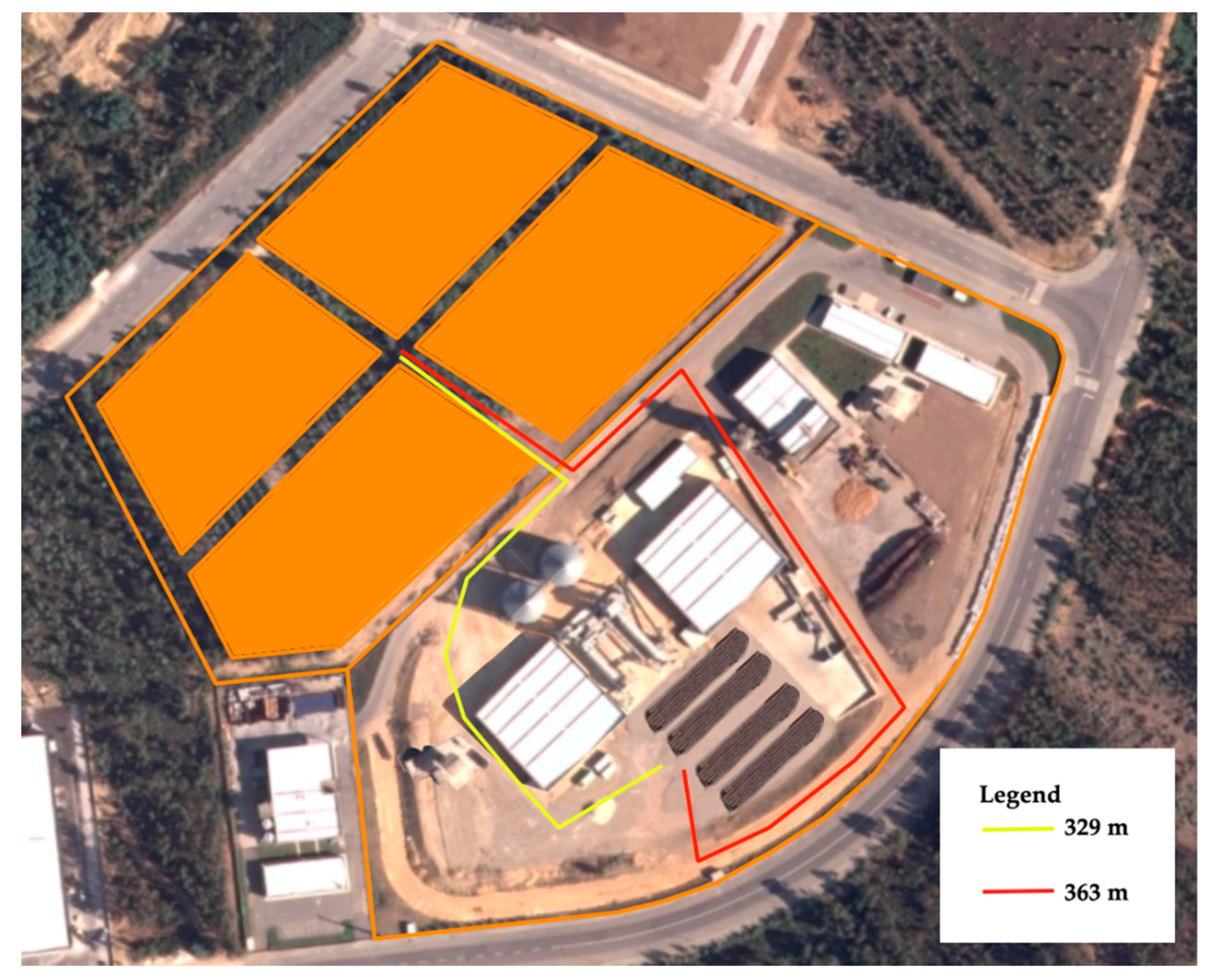
The ideal procedure for calculating T_AC would be to obtain these values by analyzing a real situation, collecting the loading, unloading, and transport times, followed by a statistical treatment of the obtained data. As already mentioned, this is not possible. 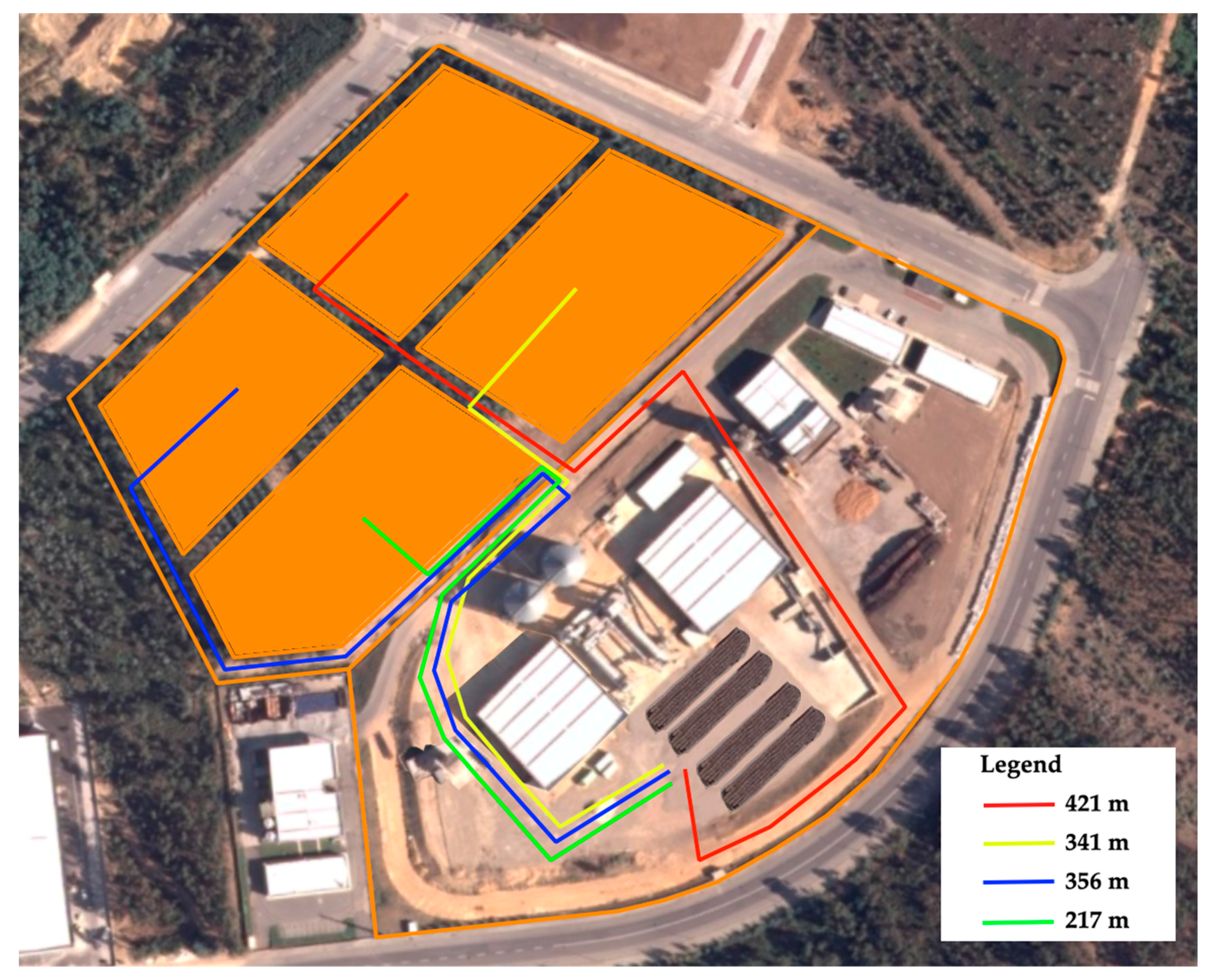For this study, the loading and unloading operations were simulated using equipment similar to what is intended to be used in the future and to what is already in operation at the industrial pilot scale production unit, Yser Green Energy SA (YGE), which occupies the P3 storage park (Figure 3). The times required for the different routes were measured with the truck loaded and unloaded making these routes. Initially, the most advantageous route for raw material transportation between P1 and P2 was determined. In Figure 3, the four sectors of P1 are represented by colored rectangles, as well as the two shorter paths to transport between the parks. As can be seen, the red route is more extensive and could cause interference with vehicles that may be in operation in P3.

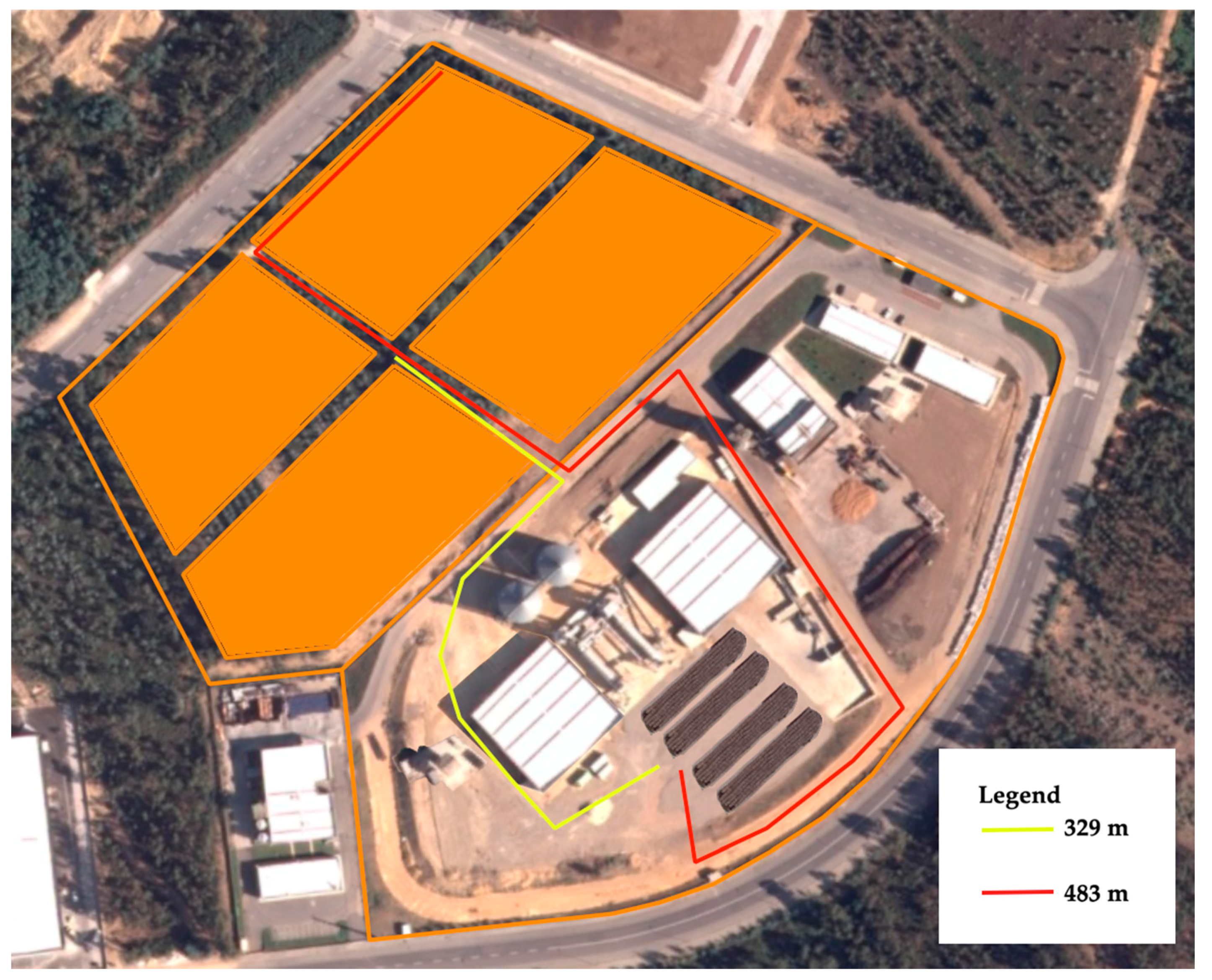
After defining the most favorable route, it is necessary to take some measurements using it as a reference. Figure 4 shows the path from the furthest point of P1 in relation to P2, colored in red, and the path from a midpoint in P1 to P2, colored in yellow, a path already used in the previous image.

One of the sectors represented by the colored rectangles will have the function of storing the biomass that will not be used by the production unit because it is not in accordance with the requirements, and consequently will not be transported to P2. If the sector chosen for this purpose is the furthest, the average course will be even lower.

Figure 5 shows the average paths for each section of P1. The distances measured in these routes are especially important for determining the differences in transport times between the four sectors and P2, which gives an idea of the significance of these differences in transport time. With the distances of the defined routes, the time for each route is determined, assuming that each transport unit moves at a speed of 20 km/h.

Using the approach shown in Figure 4, the duration of the trip will be 87 s for the red route and 60 s for the yellow route. In the same way, referring to Figure 5, the duration of the trip will be 77 s for the red route, 60 s for the yellow route, 60 s for the blue route, and 39 s for the green route.

The times obtained are not totally representative of reality and, in a real situation, would vary according to the different factors mentioned above. The factors that have more impact are related to the conditions of the route, the meteorological conditions, and the skill and performance of the TU operators. This last factor is almost impossible to evaluate, as it varies not only with the driver’s ability, which will influence the speed of the vehicle, but also with the way that drivers react to different route conditions. In turn, weather conditions and the condition of the track will influence the frictional force between the tires and the track, also contributing to variations in the vehicle speed. These issues indicate the need for statistical methods to determine the travel times. Data from a real situation over a period of time are required, in which all factors that induce relevant variations are verified. As those data were not available, values were chosen that allowed a considerable range of variation, with the awareness that this method implies obtaining a non-ideal solution.

After all these considerations, the calculation procedure can be presented as follows:

• Number of TUs needed

As a starting point, the number of trucks not capable of self-unloading that are expected to be received per day at P1 will be used to calculate the number of TUs (NTs) necessary to unload these trucks during their arrival interval:

$${\mathrm{N}}_{\mathrm{T}}=\frac{{\mathrm{N}}_{\mathrm{ETW}}\times {\mathrm{T}}_{\mathrm{U}}}{{\mathsf{\Delta }\mathrm{T}}_{\mathrm{ET}}}$$

(8)

where N_ETW is the number of external trucks without a crane, ${\mathsf{\Delta }\mathrm{T}}_{\mathrm{ET}}$ is the time interval during which external trucks are expected at P1 (min), and ${\mathrm{T}}_{\mathrm{U}}$ is the time it takes each external truck without a crane (ETW) to be unloaded (min).

As the number of TUs belonging to a given fleet cannot be a fraction, the result obtained by Equation (8) must be rounded to the next integer value. This rounding implies that there will be over-dimensioning of the fleet, and, consequently, the total time the fleet takes to unload all external trucks will be less than ${\mathsf{\Delta }\mathrm{t}}_{\mathrm{ET}}$. Thus, from the moment when there is no ET waiting to be unloaded, the TUs will have the function of transporting biomass between the parks.

• Time available for transport of biomass between parks

The next step is to obtain the time available for transport between the two parks (T_UP1). The fleet will be in operation 24 h a day, with three shifts. The TUs will mostly perform the discharge function at P1 during two of the shifts, while the transport operation between the parks will be performed on the last shift of the day and whenever the TUs are not being used at P1 during the other shifts. Therefore, it is necessary to determine the total time during the first two shifts that is not used by TUs to unload at P1. First, we determine the usage time, in minutes, of each TU at P1 (t_UP1):

$${\mathrm{T}}_{\mathrm{UP}1}=\frac{{\mathrm{N}}_{\mathrm{ETW}}\times {\mathrm{T}}_{\mathrm{U}}}{{\mathrm{N}}_{\mathrm{T}}} \left[\min \right]$$

(9)

where N_ETW is the number of external trucks without a crane, ${\mathrm{t}}_{\mathrm{U}}$ is the time it takes each ETW to be unloaded by a T_U (min), and N_T is the number of TUs.

Then, the available time for transporting raw material between the two parks is calculated as follows:

$${\mathrm{T}}_{\mathrm{TP}}=\left({\mathrm{N}}_{\mathrm{S}}\times {\mathrm{T}}_{\mathrm{S}}-{\mathrm{T}}_{\mathrm{UP}1}\right) \left[\min \right]$$

(10)

where T_S is the duration of a shift (min) and N_S is the number of shifts.

• Potential amount of biomass to be transported between parks

The last step of the first iteration is to determine the potential amount of biomass to be transported (PBT), in tons, during the total time for transport between the parks by the following equation:

$$\mathrm{PBT}=\frac{{\mathrm{T}}_{\mathrm{TP}}}{{\mathrm{T}}_{\mathrm{AC}}}\times {\mathrm{C}}_{\mathrm{T}}\times {\mathrm{N}}_{\mathrm{T}}\times {\mathrm{E}}_{\max } \left[\mathrm{t}\right]$$

(11)

where T_TP is the time available for transporting raw material between parks (min), T_AC is the average cycle time (min), N_T is the number of TUs, and E_max is the TU efficiency. The average cycle time includes the round trip, the loading time, and the discharge time, in minutes. The Emax that must be defined takes into account what was described in Section 2.2.4.

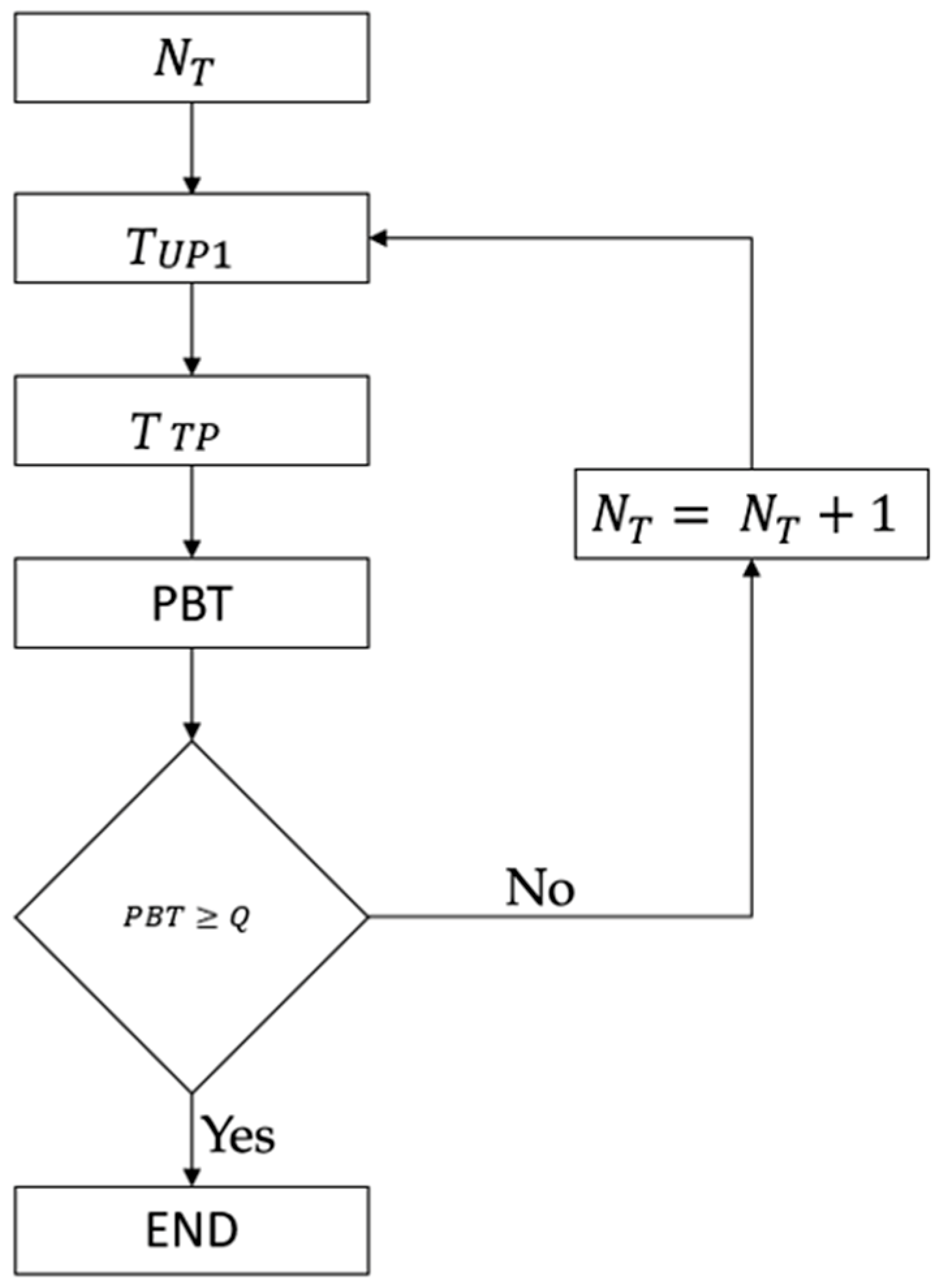
Based on these calculations, the value of the PBT is compared with the daily requirement of the production line. If the PBT value is lower than the daily requirement, a new iteration is necessary. In this new iteration, the only difference is the increment of one unit in the truck fleet relative to the previous iteration. This process is repeated continuously until the potential amount of biomass to be transported from one park to the other equals or exceeds the daily consumption of the production line.

Figure 6 shows a flowchart with the sequence of essential calculations to determine the required NT. In addition to these, there are other important calculations for the characteristics and capacities of the fleet, which will be presented next.

• Time not used by the fleet

If the condition PBT ≥ Q is verified, the next step is to calculate the total time not used by the fleet (t_NU); that is, the period of immobilization of the TUs because they have no tasks to perform. t_NU can be calculated by a variation of Equation (11):

$${\mathrm{T}}_{\mathrm{NU}}=\frac{\mathrm{PBT}-\mathrm{Q}}{{\mathrm{C}}_{\mathrm{C}}\times {\mathrm{N}}_{\mathrm{c}}\times {\mathrm{E}}_{\max }}\times {\mathrm{T}}_{\mathrm{CM}} \left[\min \right]$$

(12)

where PBT is the potential amount of biomass to be transported (t), Q is the daily requirement of the production line (t), C_C is the TU capacity (t), N_C is the number of TUs, E_max is the TU efficiency, and T_AC is the average cycle time (min).

For the system to be as optimized as possible, the result obtained with this equation must be zero. It is simple to deduce that the longer the TUs are stopped, the higher the cost of operating them because they are not producing value.

• Maximum amount unloaded by the fleet at P1

Knowing the number of trucks that make up the fleet, it is possible to determine the maximum amount unloaded by the available fleet (MAUF), in tons, during the interval ${\mathsf{\Delta }\mathrm{T}}_{\mathrm{ET}}$:

$$\mathrm{MAUF}=\frac{{\mathsf{\Delta }\mathrm{T}}_{\mathrm{ET}}}{{\mathrm{T}}_{\mathrm{d}}}\times {\mathrm{N}}_{\mathrm{T}}\times {\mathrm{C}}_{\mathrm{ET}} \left[\mathrm{t}\right]$$

(13)

where CET is the ET capacity (t), ${\mathsf{\Delta }\mathrm{T}}_{\mathrm{ET}}$ is the time interval when external trucks are expected at P1 (min), ${\mathrm{T}}_{\mathrm{U}}$ is the time for each ETW to be unloaded by a TU (min), and NT is the number of TUs.

It may also be of use to know the maximum number of trucks to be unloaded by the fleet during the interval ${\mathsf{\Delta }\mathrm{T}}_{\mathrm{ET}}$. Knowing the MAUF, we can divide this value by the capacity of the external trucks. These data may be relevant in a case where there is a need, on one or more days, to receive the maximum amount of biomass that the available fleet can process at P1.

3. Results and Discussion

3.1. Parameters Obtained for the Case Study

Applying the developed methodology requires that all data inherent in the process were collected.

Table 2. Unloading data for P1.

External Truck Capacity (t)	25
Unloading time for each truck (min)	23
Positioning time (min)	2
Truck unloading start time	07:00
Truck unloading stop time	18:00

presents the data for truck discharge at P1.

The capacity of the external trucks is the average capacity, in tons, of the trucks that transport raw material from outside to P1. Each truck’s discharge time is the time it takes to fully discharge an external truck. The positioning time is the time from the moment an external truck is unloaded until the beginning of the unloading of the next truck. The start and stop time of unloading corresponds to the time interval during which trucks carrying raw material from the outside are expected to arrive.

Table 3. Data on the transport between parks.

Transport unit capacity (t)	16
Trip time (min)	3
Unloading/loading time (min)	11

shows the material transport data from P1 to P2.

The capacity of each TU in the fleet is presented in tons. The trip time was calculated according to what was presented in Section 2.2.4, considering that the time is identical in both directions. Although the outward journey to P2 is made with the TU fully loaded and the return is made without load, the speed considered will be practicable on both trips as long as the ground is in good condition. In Section 2, the average time calculated was 1 min. However, this does not take into account the truck positioning maneuvers next to the stacks or the operator performance of TUs; thus, to account for these factors, a trip time of 3 min in each direction was used. The loading and unloading time correspond to one of these operations and not to the sum of the two. In addition to the data presented in the previous tables, it was also considered that each shift had a useful time of 420 min, and in each day, there were three shifts.

The only thing that remains to be mentioned is the daily number of ETs that need to be unloaded by the fleet to be dimensioned. This number will vary from day to day. However, we considered an average value. We estimated that P1 will receive 300,000 tons of biomass per year, equivalent to approximately 1100 tons per day, and thus 45 trucks per day were expected at P1. For every three trucks, two will not have the self-discharge capacity, and so we can conclude that, on average, every day, 30 trucks will arrive that need the help of the TUs of the fleet to perform the unloading task. However, it is important to know how the various parameters of the algorithm vary with high N_ETW variations. This is because the price fluctuations of the raw material imply that there will be times of the year when the total number of trucks received and unloaded per day varies considerably.

3.2. Application of the Algorithm Under Variable Conditions of Maximum Efficiency and Fulfilling the Needs of the Production Unit

3.2.1. Conditions: E_max = 1 and Q = 864 t/day

The algorithm was applied on the condition that 100% efficiency of the trucks is not real and, therefore, cannot be explored; however, exploring it allows us to understand the impact of the TU yield in the final decision.

The consumption of 854 tons per day corresponds to the amount of biomass that the production unit can process if it is active for three shifts, assuming that 36 tons of biomass per hour are consumed. Later, we will also consider a situation in which it is only active for two turns, avoiding operation during the night shift due to concerns with nighttime noise.

Table 4. Results for E = 1 and daily biomass amount required for the production line (Q) = 854 t.

NETW	NT	TUP1 (min)	TTP (min)	PBT (t)	MUP (t)	TNU (min)
15	1	360	900	514.3	375	−612
16	1	384	876	500.6	400	−636
17	1	408	852	486.9	425	−660
18	1	432	828	473.1	450	−684
19	1	456	804	459.4	475	−708
20	1	480	780	445.7	500	−732
21	1	504	756	432.0	525	−756
22	1	528	732	418.3	550	−780
23	1	552	708	404.6	575	−804
24	1	576	684	390.9	600	−828
25	1	600	660	377.1	625	−852
26	1	624	636	363.4	650	−876
27	1	648	612	349.7	675	−900
28	2	336	924	1056.0	700	168
29	2	348	912	1042.3	725	156
30	2	360	900	1028.6	750	144
31	2	372	888	1014.9	775	132
32	2	384	876	1001.1	800	120
33	2	396	864	987.4	825	108
34	2	408	852	973.7	850	96
35	2	420	840	960.0	875	84
36	2	432	828	946.3	900	72
37	2	444	816	932.6	925	60
38	2	456	804	918.9	950	48
39	2	468	792	905.1	975	36
40	2	480	780	891.4	1000	24
41	2	492	768	877.7	1025	12
42	2	504	756	864.0	1050	0
43	2	516	744	850.3	1075	−12
44	2	528	732	836.6	1100	−24
45	2	540	720	822.9	1125	−36

presents the results for the first iteration of the algorithm under the conditions of the study. The rows show the values of the relevant parameters that were calculated using the data defined in Section 2 where the only parameter that varies is the number of ETs that need to be unloaded by the TUs. As mentioned in that section, on average, 30 trucks of this type will arrive at P1; however, it is important to apply the algorithm to a wide range of N_ETW values.

The column corresponding to PBT should receive greater attention, particularly in occurrences where the value is close to 864 t. The greater this proximity, the more optimized the system, as this implies that T_NU will be as close to zero as possible.

If the N_ETW is 42, T_NU will be zero. This indicates that the TUs will always be up and running and that there is no time gap where they will be stopped due to a lack of tasks. When the N_ETW is 30, the TUs have a downtime of approximately two and a half hours, which is far from ideal.

The value of MUP corresponds to the raw material unloaded at P1 by the ETW; thus, it only depends on the N_ETW and the capacity of the ETW. Finally, for a N_ETW of less than 27, a second iteration of the algorithm is required as the PBT falls far short of satisfying Q.

3.2.2. Conditions: E_max = 0.84 and Q = 864 t/day

The condition to be studied is now representative of a more realistic situation in which we avoid the ideal situation, although this value still represents excellent working conditions and mechanical efficiency according to Table 1.

Table 5. Results for E = 0.84 and Q = 854 t.

NETW	NT	TUP1 (min)	TTP (min)	PBT (t)	MUP (t)	TNU (min)
15	1	360	900	432.0	375	−900
16	1	384	876	420.5	400	−924
17	1	408	852	409.0	425	−948
18	1	432	828	397.4	450	−972
19	1	456	804	385.9	475	−996
20	1	480	780	374.4	500	−1020
21	1	504	756	362.9	525	−1044
22	1	528	732	351.4	550	−1068
23	1	552	708	339.8	575	−1092
24	1	576	684	328.3	600	−1116
25	1	600	660	316.8	625	−1140
26	1	624	636	305.3	650	−1164
27	1	648	612	293.8	675	−1188
28	2	336	924	887.0	700	24
29	2	348	912	875.5	725	12
30	2	360	900	864.0	750	0
31	2	372	888	852.5	775	−12
32	2	384	876	841.0	800	−24
33	2	396	864	829.4	825	−36
34	2	408	852	817.9	850	−48
35	2	420	840	806.4	875	−60
36	2	432	828	794.9	900	−72
37	2	444	816	783.4	925	−84
38	2	456	804	771.8	950	−96
39	2	468	792	760.3	975	−108
40	2	480	780	748.8	1000	−120
41	2	492	768	737.3	1025	−132
42	2	504	756	725.8	1050	−144
43	2	516	744	714.2	1075	−156
44	2	528	732	702.7	1100	−168
45	2	540	720	691.2	1125	−180

presents the results for the first iteration of the algorithm for the conditions under study.

Under the present conditions, for an N_ETW of 30, a fleet composed of two TUs would be the ideal solution since we have T_NU equal to zero. Only for an N_ETW equal to 28, 29 or 30 is the condition PBT ≥ Q satisfied, and a new iteration of the algorithm is therefore imperative, obtaining

Table 6. Results for the second iteration E = 0.84 and Q = 854 t.

NETW	NT	TUP1 (min)	TTP (min)	PBT (t)	MUP (t)	TNU (min)
15	2	180	1080	1036.8	375	180
16	2	192	1068	1025.3	400	168
17	2	204	1056	1013.8	425	156
18	2	216	1044	1002.2	450	144
19	2	228	1032	990.7	475	132
20	2	240	1020	979.2	500	120
21	2	252	1008	967.7	525	108
22	2	264	996	956.2	550	96
23	2	276	984	944.6	575	84
24	2	288	972	933.1	600	72
25	2	300	960	921.6	625	60
26	2	312	948	910.1	650	48
27	2	324	936	898.6	675	36
28	2	336	924	887.0	700	24
29	2	348	912	875.5	725	12
30	2	360	900	864.0	750	0
31	3	248	1012	1457.3	775	412
32	3	256	1004	1445.8	800	404
33	3	264	996	1434.2	825	396
34	3	272	988	1422.7	850	388
35	3	280	980	1411.2	875	380
36	3	288	972	1399.7	900	372
37	3	296	964	1388.2	925	364
38	3	304	956	1376.6	950	356
39	3	312	948	1365.1	975	348
40	3	320	940	1353.6	1000	340
41	3	328	932	1342.1	1025	332
42	3	336	924	1330.6	1050	324
43	3	344	916	1319.0	1075	316
44	3	352	908	1307.5	1100	308
45	3	360	900	1296.0	1125	300

.

From this table, we concluded that the use of a fleet of two TUs was the most appropriate solution, since, in addition to be the ideal solution when the N_ETW is equal to 30, on days when the N_ETW is slightly lower, the downtime of the TUs will be small.

To receive 31 or more trucks to be unloaded on the same day and to satisfy the condition PBT ≥ Q, a fleet of three TUs is required, which implies a very long period when the TUs would be stopped, which is, therefore, not a viable option. However, three TUs would never be needed, since, if we consider that there will be days when the N_ETW is greater than 30, this also implies that there will be other days when the N_ETW will be below that number, thus allowing the biomass deficit transported from P1 to P2 in the first situation to be compensated when the second occurs.

3.2.3. Conditions: E_max = 0.84 and Q = 576 t/day

We next considered whether the production unit only worked for two shifts. Assuming the same processing capacity of 36 tons of biomass per hour, we reach a value of Q of 576 tons per day. In the first algorithm iteration for the conditions under study, most of the obtained PBT values do not satisfy the condition PBT ≥ Q; therefore,

Table 7. Results for the second iteration with E = 0.84 and Q = 576 t.

NETW	NT	TUP1 (min)	TTP (min)	PBT (t)	MUP (t)	TNU (min)
15	2	180	1080	1036.8	375	480
16	2	192	1068	1025.3	400	468
17	2	204	1056	1013.8	425	456
18	2	216	1044	1002.2	450	444
19	2	228	1032	990.7	475	432
20	2	240	1020	979.2	500	420
21	2	252	1008	967.7	525	408
22	2	264	996	956.2	550	396
23	2	276	984	944.6	575	384
24	2	288	972	933.1	600	372
25	2	300	960	921.6	625	360
26	2	312	948	910.1	650	348
27	2	324	936	898.6	675	336
28	2	336	924	887.0	700	324
29	2	348	912	875.5	725	312
30	2	360	900	864.0	750	300
31	2	372	888	852.5	775	288
32	2	384	876	841.0	800	276
33	2	396	864	829.4	825	264
34	2	408	852	817.9	850	252
35	2	420	840	806.4	875	240
36	2	432	828	794.9	900	228
37	2	444	816	783.4	925	216
38	2	456	804	771.8	950	204
39	2	468	792	760.3	975	192
40	2	480	780	748.8	1000	180
41	2	492	768	737.3	1025	168
42	2	504	756	725.8	1050	156
43	2	516	744	714.2	1075	144
44	2	528	732	702.7	1100	132
45	2	540	720	691.2	1125	120

presents only the results of the second iteration.

In this case, by a quick analysis of the T_NU column, we can easily discern that the solution is far from ideal. A fleet composed of only one TU is not sufficient; however, increasing the fleet by one unit means there will be huge intervals when the fleet is totally stopped. In the situation where the N_ETW is 30, there would be a 5 h interval when the TU is stopped.

Considering these results, it is pertinent to consider the possibility of adding a TU, and instead of having three shifts, to have only two. This option is implemented in the algorithm, and the results of this third iteration are presented in

Table 8. Results of the third iteration with E = 0.84 and Q = 576 t with the fleet working two shifts.

NETW	NT	TUP1 (min)	TTP (min)	PBT (t)	MUP (t)	TNU (min)
15	2	180	660	633.6	375	60
16	2	192	648	622.1	400	48
17	2	204	636	610.6	425	36
18	2	216	624	599.0	450	24
19	2	228	612	587.5	475	12
20	2	240	600	576.0	500	0
21	3	168	672	967.7	525	272
22	3	176	664	956.2	550	264
23	3	184	656	944.6	575	256
24	3	192	648	933.1	600	248
25	3	200	640	921.6	625	240
26	3	208	632	910.1	650	232
27	3	216	624	898.6	675	224
28	3	224	616	887.0	700	216
29	3	232	608	875.5	725	208
30	3	240	600	864.0	750	200
31	3	248	592	852.5	775	192
32	3	256	584	841.0	800	184
33	3	264	576	829.4	825	176
34	3	272	568	817.9	850	168
35	3	280	560	806.4	875	160
36	3	288	552	794.9	900	152
37	3	296	544	783.4	925	144
38	3	304	536	771.8	950	136
39	3	312	528	760.3	975	128
40	3	320	520	748.8	1000	120
41	3	328	512	737.3	1025	112
42	3	336	504	725.8	1050	104
43	3	344	496	714.2	1075	96
44	3	352	488	702.7	1100	88
45	3	360	480	691.2	1125	80

.

Looking at the table, we can see that there is a clear improvement in the period of non-use of the fleet. In the situation where the N_ETW is 30, there is a reduction in the time of non-use to 1 h and 40 min; however, a higher initial investment is needed.

4. Conclusions

Looking at the results, it can be concluded that the efficiency of the TUs considerably affects their performance. In a situation considering optimal working conditions and mechanical availability, this corresponds to an efficiency of 84%. That is, in a situation where there is a lack of maintenance of both the floor of the route and the TUs, the efficiency would be much less than in the situation explored and the results could be catastrophic. Therefore, it is extremely important that the floor of the path used by the TUs must be always in excellent condition, and the same applies to the mechanical state of the TUs.

The conditions studied in Section 3.2.2 produced the best solution. On average, 30 ETWs are expected, and, for this value, the algorithm produced an ideal result. In reality, we cannot count on an ideal; however, it is possible to conclude without any doubt that, for 30 ETWs arriving at P1 and for a Q of 864 t, the fleet must have two TUs to assure that the fleet is used to its maximum advantage. Section 3.2.3 explored the situation where the production unit only worked for two shifts, which implied a decrease in the amount of biomass that must be transported to P2.

For 30 ETWs, the result obtained was not satisfactory, which led to the study of a situation where the TUs would only work for two shifts, knowing that, as a result, more TUs would be required. The results obtained were substantially better, but still far from what was desired. This improvement entailed a higher initial cost, as more TUs would be needed than in the situation with three shifts. In conclusion, it is possible to affirm that the main objective of the paper was reached with a method for sizing the fleet that produced quite satisfactory results.

The transposition of the model used in the mining and quarrying industry to the biomass industry has proved to be possible and presents itself as a useful tool for the optimization of processes. Its range of application must also be tested in other scenarios, with different degrees of complexity, in order to validate its efficiency.

References

1. Le, M.T.; Nguyen, T.T.; Nguyen, T.K.N.; Do, H.T. Can Natural Gas Play an Important Role in the Energy Transition in Asia in the Future? Eurasian J. Bus. Manag. 2019, 7, 28–36. [Google Scholar] [CrossRef]
2. Zou, C.; Zhao, Q.; Zhang, G.; Xiong, B. Energy revolution: From a fossil energy era to a new energy era. Nat. Gas Ind. B 2016, 3, 1–11. [Google Scholar] [CrossRef] [Green Version]
3. Nematollahi, O.; Hoghooghi, H.; Rasti, M.; Sedaghat, A. Energy demands and renewable energy resources in the Middle East. Renew. Sustain. Energy Rev. 2016, 54, 1172–1181. [Google Scholar] [CrossRef]
4. Kabir, E.; Kumar, P.; Kumar, S.; Adelodun, A.A.; Kim, K.-H. Solar energy: Potential and future prospects. Renew. Sustain. Energy Rev. 2018, 82, 894–900. [Google Scholar] [CrossRef]
5. Nosratabadi, S.M.; Hooshmand, R.-A.; Gholipour, E. A comprehensive review on microgrid and virtual power plant concepts employed for distributed energy resources scheduling in power systems. Renew. Sustain. Energy Rev. 2017, 67, 341–363. [Google Scholar] [CrossRef]
6. Das, P.; Mathur, J.; Bhakar, R.; Kanudia, A. Implications of short-term renewable energy resource intermittency in long-term power system planning. Energy Strategy Rev. 2018, 22, 1–15. [Google Scholar] [CrossRef]
7. Gowrisankaran, G.; Reynolds, S.S.; Samano, M. Intermittency and the value of renewable energy. J. Political Econ. 2016, 124, 1187–1234. [Google Scholar] [CrossRef] [Green Version]
8. Zheng, Y.; Jenkins, B.M.; Kornbluth, K.; Træholt, C. Optimization under uncertainty of a biomass-integrated renewable energy microgrid with energy storage. Renew. Energy 2018, 123, 204–217. [Google Scholar] [CrossRef] [Green Version]
9. Nunes, L.J. Torrefied Biomass as an Alternative in Coal-Fueled Power Plants: A Case Study on Grindability of Agroforestry Waste Forms. Clean Technol. 2020, 2, 270–289. [Google Scholar] [CrossRef]
10. Nunes, L.; Causer, T.; Ciolkosz, D. Biomass for energy: A review on supply chain management models. Renew. Sustain. Energy Rev. 2020, 120, 109658. [Google Scholar] [CrossRef]
11. Nian, V. The carbon neutrality of electricity generation from woody biomass and coal, a critical comparative evaluation. Appl. Energy 2016, 179, 1069–1080. [Google Scholar] [CrossRef]
12. Nunes, L.; Matias, J.; Catalão, J. Biomass in the generation of electricity in Portugal: A review. Renew. Sustain. Energy Rev. 2017, 71, 373–378. [Google Scholar] [CrossRef]
13. Jaloliddinova, N.D.; Sultonov, R.A. Renewable sources of energy: Advantages and disadvantages. Дocтижeния нayки и oбpaзoвaния 2019, 8, 49. [Google Scholar]
14. Nunes, L.J.; Godina, R.; Matias, J.C.; Catalão, J.P. Evaluation of the utilization of woodchips as fuel for industrial boilers. J. Clean. Prod. 2019, 223, 270–277. [Google Scholar] [CrossRef]
15. Pradhan, P.; Mahajani, S.M.; Arora, A. Production and utilization of fuel pellets from biomass: A review. Fuel Process. Technol. 2018, 181, 215–232. [Google Scholar] [CrossRef]
16. García, R.; Gil, M.; Rubiera, F.; Pevida, C. Pelletization of wood and alternative residual biomass blends for producing industrial quality pellets. Fuel 2019, 251, 739–753. [Google Scholar] [CrossRef]
17. Proskurina, S.; Junginger, M.; Heinimö, J.; Vakkilainen, E. Global biomass trade for energy—Part 1: Statistical and methodological considerations. Biofuels Bioprod. Biorefin. 2019, 13, 358–370. [Google Scholar] [CrossRef]
18. Proskurina, S.; Heinimö, J.; Schipfer, F.; Vakkilainen, E. Biomass for industrial applications: The role of torrefaction. Renew. Energy 2017, 111, 265–274. [Google Scholar] [CrossRef]
19. Proskurina, S.; Junginger, M.; Heinimö, J.; Tekinel, B.; Vakkilainen, E. Global biomass trade for energy—Part 2: Production and trade streams of wood pellets, liquid biofuels, charcoal, industrial roundwood and emerging energy biomass. Biofuels Bioprod. Biorefin. 2019, 13, 371–387. [Google Scholar] [CrossRef]
20. Sandro, N.; Agis, P.; Gojmir, R.; Vlasta, Z.; Müslüm, A. Using pellet fuels for residential heating: A field study on its efficiency and the users’ satisfaction. Energy Build. 2019, 184, 193–204. [Google Scholar] [CrossRef]
21. Nunes, L.; Matias, J.C.; Catalao, J.P. Wood pellets as a sustainable energy alternative in Portugal. Renew. Energy 2016, 85, 1011–1016. [Google Scholar] [CrossRef]
22. Nunes, L.J.R.; Meireles, C.I.R.; Pinto Gomes, C.J.; de Almeida Ribeiro, N.M.C. Socioeconomic Aspects of the Forests in Portugal: Recent Evolution and Perspectives of Sustainability of the Resource. Forests 2019, 10, 361. [Google Scholar] [CrossRef] [Green Version]
23. Nunes, L.J.; Godina, R.; Matias, J.C.; Catalão, J.P. Economic and environmental benefits of using textile waste for the production of thermal energy. J. Clean. Prod. 2018, 171, 1353–1360. [Google Scholar] [CrossRef]
24. Nunes, L.J.R.; Godina, R.; Matias, J.C.d.O. Technological Innovation in Biomass Energy for the Sustainable Growth of Textile Industry. Sustainability 2019, 11, 528. [Google Scholar] [CrossRef] [Green Version]
25. Rodrigues, A.; Gonçalves, A.B.; Casquilho, M.; Gomes, A.A. A GIS-based evaluation of the potential of woody short rotation coppice (SRC) in Portugal aiming at co-firing and decentralized co-generation. Biomass Bioenergy 2020, 137, 105554. [Google Scholar] [CrossRef]
26. Nunes, L.J.; Matias, J.C. Biomass Torrefaction as a Key Driver for the Sustainable Development and Decarbonization of Energy Production. Sustainability 2020, 12, 922. [Google Scholar] [CrossRef] [Green Version]
27. Loureiro, L.; Nunes, L.; Rodrigues, A.M. Woody biomass torrefaction: Fundamentals and potential for Portugal. Silva Lusit. 2017, 25, 35–63. [Google Scholar]
28. Botelho de Miranda, H. Sincronismo de Operação e Produtividade Máxima como Critérios para Dimensionamento de Frotas Mínimas de Carga e Transporte em Contextos Mineiros e Afins; Lição de Síntese—Provas de Agregação; Universidade do Porto: Porto, Portugal, 2005. [Google Scholar]
29. De Miranda, H.B.; Leite, A. Análise de Sistemas de Carga e Transporte-Uma Abordagem Determinística. 1996. Available online: https://sigarra.up.pt/icbas/en/pub_geral.pub_view?pi_pub_base_id=215542 (accessed on 10 October 2019).
30. Leite, A. Uma Metodologia de Análise da Dinâmica de Transportes e Armazenamento. 1994. Available online: https://repositorio-aberto.up.pt/handle/10216/107648 (accessed on 10 October 2019).
31. Leite, A. Simulação como meio de obtenção de critérios para dimensionamento de sistemas de transporte e armazenamento em lavra a céu aberto. X Encontro Nac. Dos Eng. De Minas 1990. Available online: https://repositorio-aberto.up.pt/handle/10216/107242 (accessed on 10 October 2019).
32. Miranda, H.S.B.D. Transportes Mineiros: Efeitos Peculiares da Disciplina de Fecho do Relevo. 1986. Available online: https://repositorio-aberto.up.pt/handle/10216/11676 (accessed on 10 October 2019).
Figure 1. Advanced Fuel Solutions SA (AFS) facilities, where Area 1 corresponds to a plot of land of 42,000 m2 and Area 2 corresponds to a plot of land of 40,000 m2. P1 corresponds to a 2500-m2 raw material storage park that supports the experimental pilot unit; P2 corresponds to a raw material storage park of approximately 7500 m2 that serves for the production support stock; and P3 corresponds to a 40,000 m2 storage park that serves as a strategic storage stock, with a capacity for 3 months of production. (1) Social building; (2) R&D department; (3) pilot-industrial scale production unit; (4) maintenance building and parts warehouse; (5) raw material pre-processing section; (6) biomass drying and torrefaction unit; (7) densification section; (8) armed fire network of the industrial scale production unit; (9) finished product silos; (10) ordinance and scale; and (11) armed fire network of the pilot-industrial scale production unit.
Energies 13 05512 g001
Figure 2. Representation of the cycle of each transport unit (TU).
Energies 13 05512 g002
Figure 3. Representation of two possible routes for transport between parks, indicated by yellow and red lines.
Energies 13 05512 g003
Figure 4. Representation of the worst-case route (in red) and average route (in yellow) between the two parks.
Energies 13 05512 g004
Figure 5. Representation of the average paths between different sectors and P2.
Energies 13 05512 g005
Figure 6. Representative algorithm flowchart.
Energies 13 05512 g006