Article

Longitudinal Actuated Abdomen Control for Energy Efficient Flight of Insects

1
UniSA STEM, University of South Australia, Adelaide 5095, Australia
2
Department of Aerospace Engineering, Faculty of Engineering, Universiti Putra Malaysia, Selangor 43400, Malaysia
3
Joint and Operations Analysis Division, Defence Science and Technology Group, Melbourne 3207, Australia
*
Author to whom correspondence should be addressed.
Energies 2020, 13(20), 5480; https://doi.org/10.3390/en13205480
Submission received: 14 September 2020 / Revised: 14 October 2020 / Accepted: 15 October 2020 / Published: 20 October 2020
(This article belongs to the Special Issue Modelling of Aerospace Vehicle Dynamics)

Abstract

:
The actuated abdomens of insects such as dragonflies have long been suggested to play a role in optimisation and control of flight. We have examined the effect of this type of actuation in the simplified case of a small fixed wing aircraft to determine whether energetic advantages exist in normal flight when compared to the cost of actuation using aerodynamic control surfaces. We explore the benefits the abdomen/tail might provide to balance level flight against trim changes. We also consider the transient advantage of using alternative longitudinal control effectors in a pull up flight maneuver. Results show that the articulated abdomen significantly reduces energy consumption and increase performance in isolated manoeuvres. The results also indicate a design feature that could be incorporated into small unmanned aircraft under particular circumstances. We aim to highlight behaviours that would increase flight efficiency to inform designers of micro aerial vehicles and to aid the analysis of insect flight behaviour and energetics.

Graphical Abstract

1. Introduction

Flight is the most demanding form of locomotion, requiring aerodynamics, weight minimisation, balance and control. The fossil record shows ancient species of flying insects with similar body shapes to modern insects, indicating a remarkably stable evolved aeronautical solution to a diverse series of circumstances and habitats. With nature providing existence proofs of enduring solutions, it is useful to examine the function of all aeromechanical aspects of these designs.
Due to the importance of the wings, less attention has been paid to the role the body shape plays in the dynamics, performance and control of insect flight. Change in body shape can potentially be used for flight control as it can change the positions of centre of mass and centre of pressure [1]. Even land animals have been observed to use body shape changes for control, including lizards and cheetahs [2,3]. In insects, strong abdominal steering reflexes have been observed as response to mechanical or visual stimuli. For instance, a study presented by [4,5] show that desert locusts (Schistocerca gregaria), in response to an angled wind stimuli during tethered flight respond with large leg and abdominal movements. Fruit flies (Drosophila melanogaster) also demonstrated similar responses to visual rotations [6,7,8]. Additionally, in response to the speed of a translating visual pattern, modulation of the vertical abdominal angle was observed in honeybees (Apis mellifera) [9]. Moths (Manduca sexta) also show strong abdominal responses to mechanical and visual rotations about pitch axis [10]. Several videos by Rüppell show several dragonfly abdominal movements during flight [11]. However, there has been little effort to quantify these effects [12,13] and no attempt to consider the flight performance implications of the mechanism in the literature. Aircraft performance in steady flight is mostly concerned with power requirements and energy consumption [14]. Energy savings in flight from an articulated abdomen/tail are likely to emerge from torques associated with cancelling an off-center mass distribution, replacing expensive aerodynamic generation of torques. Maintenance of a torque when a structure is fixed to the ground needs no energy once applied. In practice, biological muscles holding a static torque opposing a load do consume energy [15] while producing no mechanical power. When airborne, aerodynamic generation of a torque relative to the free stream is energetically expensive, ultimately leading to increased drag. A properly designed aircraft producing a torque in addition to lift in level flight is subject to higher drag, less maximum lift and requires more propulsive power to compensate for the loss.
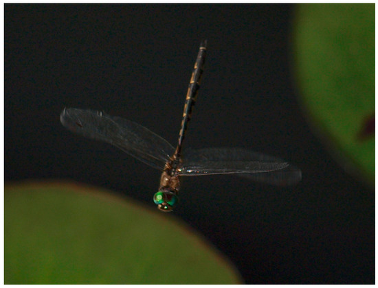
The aircraft mathematical models developed in this paper are based on biologically inspired characteristics that emulate a dragonfly (Odonata anisoptera). With two pairs of independently controlled, high aspect ratio wings and a high ratio of muscle to weight, dragonflies demonstrate superior flight performance compared to most other insect species. Dragonfly mastery of the air has been shown in a number of studies based on high speed video analysis of aerial combat and predation instances. High performance turning flight has been shown, with loads in turns exceeding 40 m/s 2 [16] and the ability to takeoff while carrying more than three times their own body weight [17]. Dragonflies have also been shown to pursue prey animals using the chasing strategies found in missiles [18] and to have exceptionally high success rates in capturing aerial prey [19,20]. It has been demonstrated that they have surprisingly efficient glide performance comparable to model aircraft with higher Reynolds numbers (Re). Observed lift-to-drag ratios range from 3.5 to over 10 [21,22,23]. Some species of dragonfly have been observed to migrate across hundreds of kilometres [24], a difficult energetic achievement for such a small organism. Energy scavenging by dragonflies has also been observed, in which they soar on thermal updrafts and on rising air currents caused by slopes [25].
The dragonfly body form is dominated by a long abdomen (weighing 31–35% of the total body mass), two pairs of comparatively high aspect ratio wings (weighing less than 2% of the total body mass), a dense thorax and a large head dominated by large eyes [26]. The dragonfly abdomen is by no means a “tail” in the normal sense for vertebrates, neither is it analogous to traditional aircraft empennage. Aircraft tails are generally rigid structures on which there are aerodynamic surfaces, both horizontal and vertical. In many species of dragonfly, there are no aerodynamic structures at the distal end of the abdomen. Figure 1a–d shows the typical abdomen shape of dragonfly families. Most dragonfly and damselfly abdomens are slender, as in Figure 1a showing the silhouette of a dragonfly from the family Aeshnidae. Variations exist, for example, some “chasers” of the family Libellulidae have a shorter thicker abdomen as shown in Figure 1b. Some “clubtails” of the family Gomphidae as shown in Figure 1c, have a pronounced club shaped structure terminating the abdomen from which the family draws its name, strengthening a hypothesis of a predominantly inertial role in this case at least. Some “petaltails” of the family Petaluridae appear to have an aerodynamic structure terminating their abdomens (Figure 1d). It might be relevant that the largest dragonfly species by some measures, Petalura ingentissima, carries such a structure.
The abdomen is certainly required to exist regardless of flight control since it contains the digestive tract and anatomical features related to reproduction. It is also required to be actuated to some extent for mating and oviposition [28], as well as the likely evolutionary requirement to be neither long and rigid or long and flexible. Thus, the cost of articulating the abdomen is only the additional muscle mass required to achieve rapid movements. Therefore, we focus on two observed abdominal motions and their utilisation for correction of imbalance in steady level flight and for a longitudinal pull up maneuver, which are:
  • Tail contraction and extension, illustrated in Figure 2a and will be referred to as “Model 1” and,
  • Tail up down wag movement, illustrated in Figure 2b and will be referred to as “Model 2”.
In the remainder of this paper we introduce the performance and dynamics model used to demonstrate and quantify the energetics of these techniques.

2. System Model

We have used the most accessible and analytical means possible for the analysis to avoid resorting to poorly understood, case specific or possibly methodological artefacts from fluid simulation. We have also focused on the case of longitudinal flight with fixed wings, which results in acceptable fidelity with a focus on wings with attached air flow and clear applicable outcomes. In demonstrating how features of dragonfly anatomy could save energy in flight, an aircraft in the well understood scale of small fixed wing models with Reynolds numbers in thousands, rather than dragonflies with Reynolds numbers in hundreds, was used. The discipline of aircraft performance contains well established methods and tools for performance estimation of fixed wing aircraft, which also yield algebraic expressions that are amenable to new derivations, optimisation and predictions. Wherever possible, algebraic expressions and conventional aerodynamic techniques were used, with the nomenclature commonly used in the aerospace literature [29,30].
For the purposes of isolating inertial from aerodynamic forces on the tail, the aerodynamic effects of the tail were ignored as these effects were expected to have little influence on the aerodynamics of the aircraft, compared to the wings, legs and thorax. A particular advantage of an inertial actuator is that it will continue to produce torques at low speeds, even when the aircraft is not flying or in an aerodynamic stall. For this reason, we might expect to see large abdominal motions at low speeds. To simplify this problem, the articulated tail was placed in the analytical framework developed for small fixed wing aircraft. Dragonflies have efficient wings, credited by Wakeling with glide slope of 6.3:1 [21]. Many documented observations of dragonflies engaging in extended periods of soaring and gliding exist [21,25,31,32], so, fixed wing cruising and gliding flight is an appropriate and accessible aspect of their flight for our analysis. Although the analysis in this study focuses on fixed wing modes of flight, the qualities of the outcomes should apply to flapping wing flight. The assumption of the analysis is that the abdomen/tail is a mass that is already present and required. We focus on the question of the potential benefits to maneuverability and energetics of the inertial tail.

2.1. Reference Frames

The aircraft is modelled as a collection of rigid bodies. The dragonfly head to thorax region, including the wings are abstracted as a rigid body B with a mass m B and will be referred to as the “body”. The abdomen, interchangeably referred to as the “tail” in this paper, is modelled as an added mass, m T , concentrated at the tip of the tail T . Reference frames used for the development of the equations of motion are defined as shown in Figure 3. The North-East-Down (NED) coordinate system which is commonly used in aeronautics is adapted for each of the Earth, body and tail [33]. The coordinates in each frame are ( X I , Y I , Z I ) , ( x B , y B , z B ) and ( x T , y T , z T ) respectively. The origin of the inertial frame (I) is fixed at an arbitrary point relative to the earth’s surface. The origin of the body-fixed frame (B) can be arbitrarily selected to be any point on the body of the aircraft. The tail reference frame (T), originates from the centre of gravity ( c g ) of the tail point mass with its orientation the same as that of the body frame coordinate system when the tail is undeflected. The whole aircraft ( b o d y + t a i l ) will be referred to as the rigid body C . In addition, four reference points, b , c , t and j are introduced. These points represent the locations of the center of mass of the body only, the whole aircraft, the tail and the tail joint location respectively.

2.2. Equations of Motion

Whilst only longitudinal flight was examined in this study, for completedness, the full non-linear dynamic model of the aircraft is presented. It is common practice to derive equations of motion referenced to the combined c g of an aircraft, however, to properly reflect the effects associated with dynamic changes in combined c g position, the dynamic equations presented in this study are referenced to point b which is the centre of mass of the rigid body B in the body-fixed reference frame B. When the reference frame of a vector or tensor is not specified, it automatically means it is written in the body-fixed reference frame B.

2.2.1. Kinematics

The translational and rotational kinematic equations for an aircraft are available in the flight dynamics literature. In matrix form, the translational kinematic equations are [29]
ε . = [ R ] I B V B I ,
where ε represents the position ( x , y , z ) of the aircraft relative to the inertial frame, [ R ] I B is the rotation matrix from body-fixed frame to inertial frame and V B I is the aircraft body velocity components ( u , v , w ) .
Since the intention is not to model very large attitude angles, the standard aerospace rotational kinematic equations using Euler angles ( ϕ , θ , ψ ) are chosen to represent the attitude of the aircraft and are given by [29]
ϕ . θ . ψ . = 1 s i n ϕ t a n θ c o s ϕ t a n θ 0 c o s ϕ s i n ϕ 0 s i n ϕ c o s θ c o s ϕ c o s θ p q r ,
where ( p , q , r ) are the body frame angular velocities of the aircraft.

2.2.2. Dynamics

Two sets of dynamic equations are developed for the two modes of tail actuation considered in this study. The first set of equations represent Model 1, which was used for modelling the contraction and extension of the dragonfly tail during flight (see Figure 2a). The second set of equations representing Model 2, was used to model the up and down wag movement of the dragonfly tail during flight, shown in Figure 2b. The equations are derived based on the following assumptions:
  • Earth is flat and non-rotating and is the inertial frame.
  • The aircraft is electrically powered, has a constant total mass but varying mass distribution.
  • The mass and mass distribution of the rigid body B remains the same throughout the flight.

Model 1 Aircraft Dynamics

The translational and rotational dynamic equations are given by Equations (3) and (4) respectively [34,35]
V . B I = 1 m F ω ˜ B I V B I 1 m m T ρ . . t b + ω ˜ B I ω ˜ B I ρ t b + 2 ρ . t b ρ ˜ t b × ω . B I ,
ω . B I = 1 J b C M 1 J b C ω ˜ B I [ J b B ] B ω B I 1 J b C ( ρ ˜ t b m T ω ¯ B I ρ t b ω B I + ρ . . t b + ρ ˜ t b m T ω ˜ B I V B I + V . B I + 2 m T ( ρ ¯ t b ρ . t b ) I ρ . t b ρ ¯ t b ω B I ) ,
where ρ t b , ρ . t b and ρ . . t b are the position, velocity and acceleration of the tail mass with respect to point b in the body frame. ω B I is the body frame angular velocity components ( p , q , r ) and m is the total mass of the aircraft. F and M represent the total forces and moments acting on the aircraft respectively.
The change in c g position with respect to point b, written in the body frame is expressed as
ρ c b = m T ρ t b m .
In addition, the inertia matrix of the whole system about point b is given by
J b C = J b B + J b T ,
where J b T is expressed as
J b T = m T ( ρ ¯ t b ρ t b ) I ρ t b ρ ¯ t b ,
and I is a 3 × 3 identity matrix.
The elements of the inertia tensor J are
[ J ] = J x x J x y J x y J y x J y y J y z J z x J z y J z z .

Model 2 Aircraft Dynamics

The translational and rotational dynamic equations are represented by Equations (9) and (10) respectively [34,35,36,37]:
V . B I = 1 m F 1 m ( m T [ [ R ] B T [ ω . T B ] T × [ ρ t j ] T + [ ω ˜ T B ] T ( [ ω ˜ T B ] T [ ρ t j ] T ) , + ω . B I × ( [ R ] B T [ ρ t j ] T + ρ j b ) + ω ˜ B I ω ˜ B I × ( [ R ] B T [ ρ t j ] T + ρ j b ) + 2 ω ˜ B I [ R ] B T ( [ ω ˜ T B ] T [ ρ t j ] T ) ] ) ω ˜ B I V B I ,
ω . B I = 1 J b C ( M [ m T [ R ] B T [ ρ t j ] T + ρ j b [ [ R ] B T [ ω . T B ] T × [ ρ t j ] T + [ ω ˜ T B ] T ( [ ω ˜ T B ] T [ ρ t j ] T ) + ω ˜ B I ω ˜ B I × ( [ R ] B T [ ρ t j ] T + ρ j b ) + 2 ω ˜ B I [ R ] B T ( [ ω ˜ T B ] T [ ρ t j ] T ) + V . B I + ω ˜ B I V B I ] ] ) ,
where [ ω T B ] T and [ ω . T B ] T are the angular velocity and acceleration of the tail mass with respect to the body frame respectively. The change in c g position and the total inertia matrix of the whole system are also estimated using Equations (5)–(7), however,
ρ t b = [ R ] B T [ ρ t j ] T + ρ j b .

2.3. Forces and Moments

The forces and moments acting on an aircraft are mainly due to aerodynamics, propulsion and gravity. In this study the same aerodynamic and propulsive models were used for both dynamic models developed. These models are well established for fixed wing aircraft in the flight dynamics literature such as [33,38] and will not be discussed in this paper. It is important, however, to note that we assume the aircraft thrust aligns with the longitudinal axis and hence, does not produce any moments.
The gravitational force model for both dynamic models are also the same and are detailed in [33], however, the gravitational moments for both tail actuation modes differ. For Model 1, the gravitational moment ( L g , M g , N g ) is
L g M g N g = ρ t b × [ R ] B I 0 0 m T g .
where g is the acceleration due to gravity. However, for the Model 2, the gravitational moment produced by the tail is given by
L g M g N g = ( [ R ] B T [ ρ t j ] T + ρ j b ) × [ R ] B I 0 0 m T g .

2.4. Control Inputs

For propulsion, the control input used in this study is the thrust ( T n ) . The aerodynamic control surfaces are the left and right elevons, denoted by η l and η r respectively and located on the trailing edges of the wings as shown in Figure 3. Generally, elevons, depending on the desired flight regime, function as elevators or ailerons. The combined deflections of the elevons as elevators δ e or ailerons δ a are according to [33]
δ e δ a = 1 1 1 1 η r η l .
With regards to the longitudinal motion of the aircraft model in this study, the two main functions of the elevators are for longitudinal trim and/or longitudinal control. When deflected, the camber of the airfoil of the wing is changed and the lift coefficient ( C L ) changes consequently. Therefore, elevator deflection increases or decreases wing lift and pitching moment [39]. The elevator deflection δ e , presented in this study is a function of the left and right elevons acting as left and right elevators respectively ( η r = δ e r and η l = δ e l ), such that
δ e = δ e r + δ e l 2 .
The tail mass linear displacement or angular deflection on the other hand, functions as an alternative moment generator, changing pitching moment [34]. For Model 1, the control inputs are the tail mass positions ( ρ t b x , ρ t b y , ρ t b z ) and for Model 2, the control inputs are the tail mass angular deflections ( ϕ T , θ T , ψ T ) relative to the body frame. Where applicable, a downward deflection of a control surface or tail deflection is positive and an upward deflection is negative.

2.5. Energy Maneuverability

Maneuverability in flight involves the ability to perform a change, or a combination of changes in, altitude, direction and airspeed [40]. As mentioned earlier, dragonflies demonstrate superior maneuverability as apex predators among insects. Energy maneuverability involves the analysis of maneuverability, expressed in terms of energy and energy rate. Although energy maneuverability is not directly concerned with electrical energy consumption, the use of appropriate energy maneuverability strategies can result in reduced electrical energy consumption.
Summing the forces acting on an aircraft, parallel to the flight path as shown in Figure 4, the velocity change equation yields [41,42],
m V . = T n D m g s i n ( γ ) ,
where γ is the flight path angle.
The total energy or energy state of an aircraft, is expressed as the sum of kinetic and potential energy,
E = 1 2 m V 2 + m g H ,
where H is the height.
To enable comparison of maneuver performance of various aircraft, it is more convenient to use the specific energy E s , which is the energy per unit mass. The specific energy is sometimes called the energy height,
E s = H + V 2 2 g .
The energy state of an aircraft can be changed by applying power. The rate of change of specific energy E . s , also known as specific excess power P s is
E . s = P s = H . + V g V . .
Using the kinematic relation that H . = V s i n ( γ ) and the expression of V . from Equation (16), Equation (19) becomes
P s = T n D W V .

3. Aircraft Model Specifications

The specifications of the aircraft model used in this study are chosen to represent an electrically powered fixed wing aircraft with a mass distribution reminiscent of a dragonfly (see Figure 3). The datum which the position values are obtained with respect to is chosen as the leading edge of the wing. The implementation of the mathematical models was carried out in the MATLAB/Simulink simulation environment [43]. Figure 5 shows the Simulink model of the aircraft. The “Actuator model” produces the control inputs to the “Aircraft model” which contains the nonlinear equations of motion to then produce the aircraft state vector ( u , v , w , p , q , r , ϕ , θ , ψ , x , y , H ) .

3.1. Physical Properties

A scaled up ( × 10 ) model of dragonfly planform parameters measured by Okamoto [44] is presented. The fore and hind wing areas are combined to form a single wing with an averaged chord ( c r e f ) . Estimating the effective aspect ratio ( A R ) of the fore and hind wing resulted in an inappropriate low value, hence, an ( A R = 7.3 ) was selected as dragonflies are characterised with having high AR wings [22,45]. We determined the value of the wing span ( b r e f ) using [14]
b r e f = A R × c r e f .
In this study, the tail mass was chosen as 0.06 kg, making it approximately 15% of the total mass of the aircraft. The maximum tail/abdominal length was chosen to be 0.4 m, which was about 1.33 × the body length. These values were chosen with consideration to the fixed wing assumption and using [26,28,44] as guides. In addition, the aircraft was assumed to be symmetrical about the x z plane, therefore, J x y = J y z = 0 . Furthermore, J x z was neglected in comparison with the moments of inertia. The physical properties of the aircraft model are summarised in Table 1.

3.2. Aerodynamic Model

XFLR5 and AVL were used to establish the aerodynamic model of the aircraft. XFLR5 extends the 2D solutions of XFOIL to 3D applications using the Vortex Lattice Method (VLM) and lifting line theory (LLT). Athena Vortex Lattice (AVL), developed by Drela, is an extended vortex-lattice tool [46,47,48]. XFLR5 and AVL produce relatively accurate aerodynamic data that has been used for real aircraft applications [49]. The Phoenix airfoil (Ph o ¨ nix) [50,51,52] was selected for this study. It is a relatively thin (thickness below 10 % ), low Reynolds number airfoil, often used in small tailless aircraft such as the solar powered flying wing UAV developed in [50]. Tailless aircraft do not possess conventional vertical stabilisers and often exhibit poor lateral dynamic stability [53]. To improve lateral stability, a positive dihedral of 3 was applied along the wing span and the wing was twisted at the root by 3 to reduce stall tendencies at the tip [53,54]. The aerodynamic characteristics of the airfoil which was evaluated in XFLR5 at R e = 10 5 is presented in Figure 6.
In addition, XFLR5 was used for the initial distribution of the point masses and initial estimation of moments of inertia of the aircraft. The aircraft AVL model shown in Figure 7 includes a fuselage, however, as recommended in the AVL documentation [55], it was excluded from the AVL model used to generate aerodynamic data. The aerodynamic data for the airframe were generated using an alpha sweep from −10 to +10 , with increments of 2 . The generated data was stored in look up tables and used in the simulation of the non-linear model in Simulink [43]. All maneuvers considered in this study assume zero sideslip β = 0 . The aerodynamic data used in the simulation were obtained with respect to an arbitrarily chosen aerodynamic reference point (ARP). Doing so enabled the aerodynamic moments at any point in the body frame to be calculated as the sum of the aerodynamic moments at the ARP and the cross product of the aerodynamic forces and corresponding lever arms Δ x b x A R P , Δ y b y A R P and Δ z b z A R P . For example, the aerodynamic moments at point b are [14]
M A e r o B = M A e r o A R P + F A e r o B × Δ x b x A R P Δ y b y A R P Δ z b z A R P .

3.3. Control Inputs

The physical constraints of the control inputs used in the simulation are shown in Table 2. The neutral position of the tail for Model 2 was considered to be when it was fully extended with no deflection and the tail angular deflection limits were relative to the neutral position.

4. Analysis and Results

The longitudinal flight analysis and results for correction of imbalance in steady cruise flight, and pull up maneuver using the two tail mass actuation modes, are presented in this section.

4.1. Longitudinal Trim for Steady State Flight

To verify the correctness of the models developed in Section 2.2.2, Models 1 and 2 were trimmed for steady level flight, given the same longitudinal positioning of the tail mass. In steady state flight, translational and rotational velocity components in body frame were constant so, u . = v . = w . = p . = q . = r . = 0 . Additionally, for the steady wings level flight condition, the body frame angular rates, p = q = r = 0 , since the Euler rates were constant. The roll angle, ( ϕ = 0 ) and we also assumed the yaw angle, ( ψ = 0 ) . Since cruise altitude was constant, z . = 0 and a y . = 0 condition was imposed. The position of the tail mass in the body frame was fixed, ρ . . t b = ρ . t b = 0 for Model 1 and ω . T B = ω T B = 0 for Model 2.
For both models, the objective was to calculate the nominal values of the pitch angle ( θ 0 ) and control inputs ( δ e 0 ) and ( T n 0 ) for cruise speed V 0 = 10 m/s and height H 0 = 100 m. In addition, there was no tail deflection ( θ T 0 = 0 ) and the tail position was fixed at ( ρ t b x 0 = 0.564 m) for both models. No tail deflection infers that for Model 2, ( ρ t j 0 = 0.264 m) and ( ρ j b 0 = 0.3 m). The models were trimmed without actuator dynamics using the Matlab/Simulink linear analysis tool [43]. The trim results are presented in Table 3.

4.2. Correction of Imbalance in Cruise Flight

An essential flight safety requirement is aircraft stability, however, imbalance during flight is caused by many factors such as wind and mass distribution errors. Balance control is mainly affected by the centre of gravity c g location of the whole aircraft and the ability of an air vehicle to correct for imbalance during steady flight is desirable. Therefore, modelling of balance and control surface effects allows analysis of efficiency in steady flight. Since the concern of this study was longitudinal balance, the c g location change experienced was mainly along X B axis we express parameters with regards to that axis from this point on. One way to determine the static longitudinal stability of an aircraft is using the static margin (SM), given by [14]
S M = X N P X c g m c r e f ,
where X N P is the neutral point (NP), X c g m is the c g position of the whole aircraft along X B axis.
Generally, if c g is ahead of the N P , then S M is positive and the aircraft is stable. The larger the S M , the more stable and less maneuverable an aircraft is. However, if the c g is behind the N P , resulting in a negative S M , the aircraft is unstable in pitch, making it difficult or impossible to fly [14]. The S M value is usually chosen based on the desired performance of the aircraft in terms of handling qualities and usually ranges from ( 10 % S M 5 % ) , for piloted aircraft. Considering the dragonfly’s high level of maneuverability, control effects of four wings and fast nervous system for control, a S M = 0 or even negative can have advantages [56,57]. There are consequences for all settings of SM, which go beyond the scope of this study.
For both tail actuation modes, the analysis was treated as an instantaneous performance problem. Therefore, the tail position ρ t b , or angular deflection θ T was known prior to the analysis, which was then used to calculate the c g m and inertia values in MATLAB/Simulink, [43] to be specific. The energy was evaluated at constant velocity in steady cruise flight. We illustrate the use of tail linear displacement to correct longitudinal imbalance as depicted in Figure 2a. To do this, an artificial physical disturbance that causes an imbalance in level flight was introduced as an added mass D , located at an arbitrarily chosen point d in the body frame. One could relate the introduction of a disturbance mass in flight as a scenario where the dragonfly caught prey during flight using mandibles or forelimbs, causing the c g m to shift forward, reducing maneuverability of the aircraft, which was undesirable. However, by changing tail mass position or angular deflection, the aircraft was able to return to the desired maneuverability prior to the addition of the disturbance mass. It should be noted that for consistency, the pre-known values of ρ t b or θ T after correction of imbalance were deliberately set in this study; the static margin after correction of imbalance was the same as that of the initially undisturbed and balanced aircraft, which was indicated by the values of the combined c g position.
The neutral point of the aircraft planform analysed in this study was estimated in AVL, as ( X N P = 0.046 m). In order to isolate the tail mass movement, rigid body B and the disturbance mass D were combined to form a rigid body A with a constant mass and mass distribution. The mass and inertia properties of the newly defined rigid body A were estimated in XFLR5 and are listed in Table 4. The traditional method to instantaneously correct imbalance or disturbance of aircraft is to use aerodynamic control surfaces to create opposing forces. We calculated the control effort ( δ e ) for Models 1 and 2, for a stable trimmable steady cruise flight condition at airspeeds ranging from (V = 5–15 m/s) with an increment of 0.5 m/s. The evaluations carried out for both tail actuation modes are described in the sections that follow. In most small electrically powered aircraft, at least 50% of the power available is used for propulsion [58], therefore, the less propulsive power consumed, the longer the aircraft can fly on less energy. For steady cruise, lift balances the gravitational force ( L = W ) and the net thrust balances the drag ( T n = D ) , therefore, the specific power is zero. The energy required E r e q in cruise as a function of time can be estimated by:
E r e q = t t f P r e q d t ,
The power required P r e q is equivalent to the energy required for 1 s in cruise. Therefore, to quantify the performance in terms of energy, we use ( P r e q = D V ) . The analysis in this section assuming that there is always sufficient thrust to overcome the drag.

4.2.1. Model 1

With this model, we examined the use of tail linear positioning to regain a balanced, energy efficient cruising flight condition after the sudden addition of an unbalanced mass. Table 5 presents a summary of the three cases considered with side view illustrations. The first case considered was the nominal undisturbed case with an initial static margin of S M M o d e l 1 = 11.8%, where the tail was initially somewhat contracted prior to the disturbance. In the second case, the disturbance mass was introduced, however, the tail was left in its initial position and played no role in correcting flight. Considering the position where the disturbance mass was added, the corrective reaction required was for mass to be moved backward by extending the tail. Therefore, the third case considered was a case where the tail was extended such that the tail mass was now halfway between the initial position and the maximum possible position in an effort to correct for imbalance.
Plots of elevator deflection to trim the aircraft and power required for the range of airspeed considered were estimated using the Matlab/Simulink linear analysis tool [43]. The results are shown in Figure 8a,b respectively and summarised in Table 6.

4.2.2. Model 2

For this model, we examined the use of tail angular deflection to regain balance in the cruising flight condition after the sudden addition of an unbalanced mass. Again, we considered three cases which are summarised in Table 7 with side view illustrations. The first case, being the nominal undisturbed case with an initial static margin of S M M o d e l 2 = 7.7%, was where the tail was deflected upwards to its maximum possible deflection angle. In the second case, the disturbance mass was added, however, the tail was left in its initially deflected position and played no role in correcting flight. Again, considering the position where the disturbance mass was added, the corrective reaction required was for the tail mass to be deflected towards its neutral position, thus increasing distance of the mass from the centre of gravity. Therefore, in the third case considered, in an effort to correct for imbalance, the tail moved to its neutral position, meaning no deflection.
Plots of elevator deflection required to trim Model 2 aircraft and power required for a range of airspeed are shown in Figure 9a,b respectively. Table 8 presents a summary of results for trimmed steady cruise for Model 2.

4.3. Pull up Maneuver

We performed a quasi-steady analysis for a pull up maneuver using Models 1 and 2. An aircraft flying initially in steady level flight at a speed V 0 was subjected to a small change in the longitudinal control effector of choice (mass shift or control surface), causing it to pull up with a corresponding quasi-steady angle of attack (AoA) α , and body pitch rate q. This was computed by enforcing ( α . = q . = 0 ) . As the pull up progressed, the airspeed and flight path angle changed at a slow rate in comparison to the AoA and pitch rate [14,59]. Traditionally, this maneuver is initiated using elevator deflection, δ e . However, as mentioned earlier, Models 1 and 2 provide alternative ways to generate pitching moment for a pull up maneuver.
In both cases, the aircraft was initially trimmed for steady level flight using the elevator before the maneuver was initiated. We defined the wings-level pull up maneuver by trajectory and estimated the additional control effort required for the same maneuver, using the elevator compared to tail linear displacement or using the elevator compared to tail angular deflection. The purpose was to compare the pull up effort using the traditional elevator to the two alternative tail actuation methods and estimate which consumes or requires more energy. As this is a maneuver, energy maneuverability is of more interest, hence, we limited this investigation to cruising power maneuvers, so Δ T n = 0 . To enable comparison, we compare the energy state and energy rate by estimating the specific energy E s , and specific excess power P s for the first 3 s after the maneuver was initiated. Since this was an open loop control analysis, the additional control effort required to achieve the same pull up trajectory in each scenario was pre-estimated in Simulink.

4.3.1. Model 1

With this model, alternative pitching moment was generated when the tail mass moved along the body x B axis (see Figure 2a). The aircraft was initially trimmed for a cruise speed of V = 10 m/s, H = 100 m and a tail mass position of ( ρ t b 0 = 0.564 m). The solutions to this trim condition for Model 1 are presented in Section 4.1 and Table 3. The load factor n = L W , associated with a pull up maneuver was selected such that the aircraft dynamic response provided a good response to capture the flight dynamics and remained within the operating regime of interest. The additional control effort required for approximately the same pull up maneuver trajectory was estimated as Δ δ e 1 . 5 using the elevator and Δ ρ t b x 0.069 m using tail linear displacement.
The simulation was run for 4 s and excitation to the control inputs was applied using a pulse for 0.25 s, 1 s into the simulation. The time history for airspeed V and trajectory H as excited by change in elevator deflection or tail linear displacement are shown in Figure 10. The specific excess power and specific energy as effected using elevator deflection or tail linear displacement are shown in Figure 11 with respect to time.
The results in terms of average specific energy and specific excess power using either elevator deflection or tail mass linear displacement for the same pull up maneuver are summarised in Table 9.

4.3.2. Model 2

With this model, the tail mass generated pitching moment by wagging the tail up and down (see Figure 2b). Table 10 shows the initial steady level flight condition values before the pull up maneuver was initiated. The additional control effort required for a similar pull up maneuver was estimated as Δ δ e = 0 . 58 using the elevator and Δ θ T = 53.5 using tail angular deflection.
For a duration of 4 s, the pull up maneuver was initiated using a pulsed input signal (applied 1 s into the simulation for 0.25 s). The time history comparisons for airspeed and trajectory are shown in Figure 12, while that for specific excess power and specific energy are shown in Figure 13. Table 11 shows a summary of the specific energy and power used in the pull up maneuver using Model 2.

5. Discussion

In this study, we have examined the effect of an inertial tail appendage on a relatively conventional fixed wing aircraft and considered performance, emphasising efficiency. For two longitudinal flight scenarios, we have shown how the abdominal movements, as observed in dragonflies, improve flight performance.

5.1. Correction of Imbalance in Steady Level Flight

It is safe to assume that passive stability for a four winged flapping craft, capable of nearly holonomic locomotion [60], is not a necessary precondition in the same way that it is for a fixed wing aircraft. Yet, the stability of the surrogate fixed wing aircraft would be adversely affected by c g m variations, as a zero or negative stability margin would lead to a departure from controlled flight.
For Models 1 and 2 aircraft and for all cases relating to correction of imbalance in steady level flight, the plots for elevator deflection required to trim with respect to airspeed are consistent; the amount of elevator deflection required to trim decreased with increased speed because higher air speeds require less lift coefficient C L and consequently less angle of attack [39]. The power required plots as a function of airspeed also present consistent results as increased weight results in more lift required and consequently, an increase in induced drag (see Figure 8 and Figure 9) [39].
Although the power required after both models were disturbed was obviously higher than the initial condition, performance improved in the form of lower power required compared to before the tail was moved to compensate for imbalance, however, the magnitude of power saved was different for each model due to the difference in initial configurations.
Specifically, for Model 1 with a linearly displaceable tail mass as in Figure 2a, an average increase in elevator deflection of 161% was observed after the disturbance mass was introduced, compared to 55% after correction of imbalance was performed by linearly extending the tail. In addition, results showed an average of 12% increase in energy required after the disturbance mass was introduced, compared to 7% after correction of imbalance was performed by linearly extending the tail.
For Model 2 with a deflectable tail as in Figure 2b, an average increase in elevator deflection of 116% was observed after the disturbance mass was introduced, compared to 46% after correction of imbalance was performed by moving the tail to its neutral position, which had zero deflection. The results showed an average of 13% increase in power required before, compared to 9% after correction of imbalance. Overall, for steady cruise, a 4–5% average in propulsive power savings is quite substantial for an electrically powered aircraft.

5.2. Pull up Maneuver

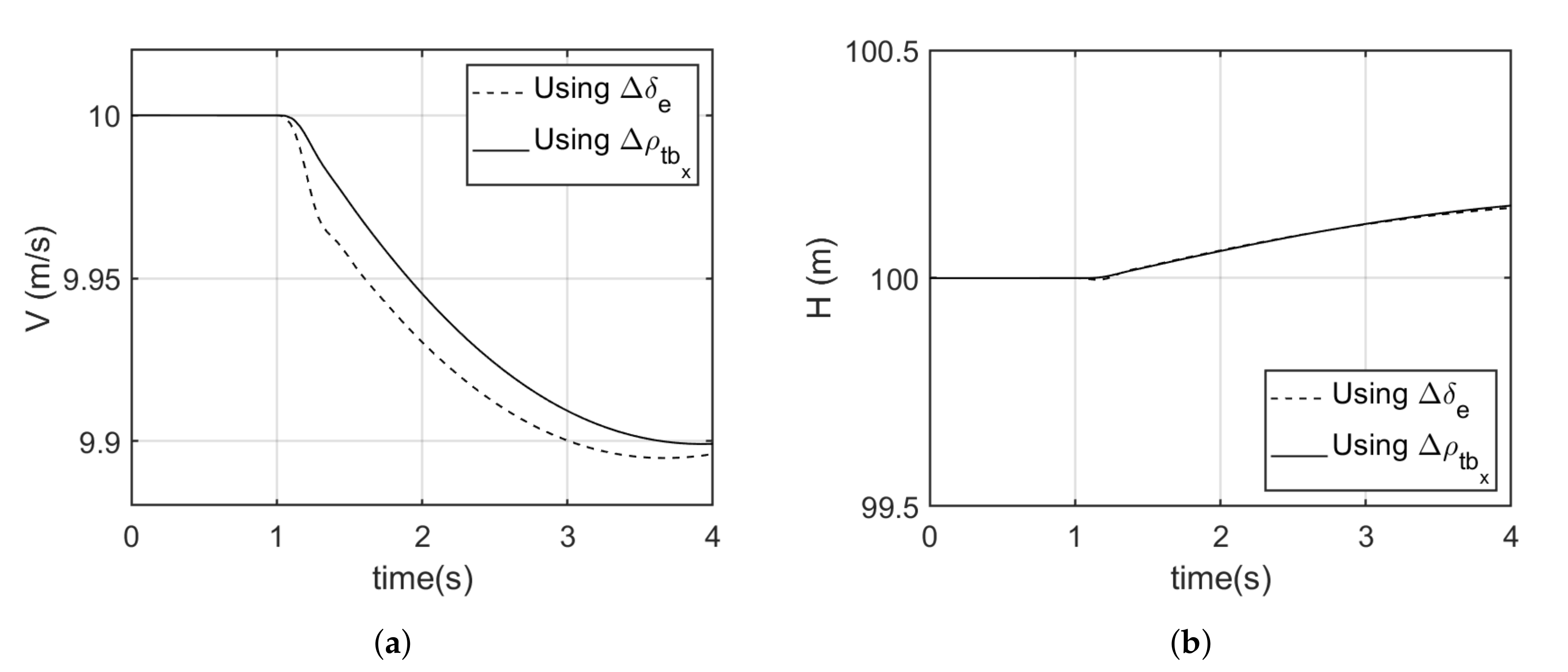
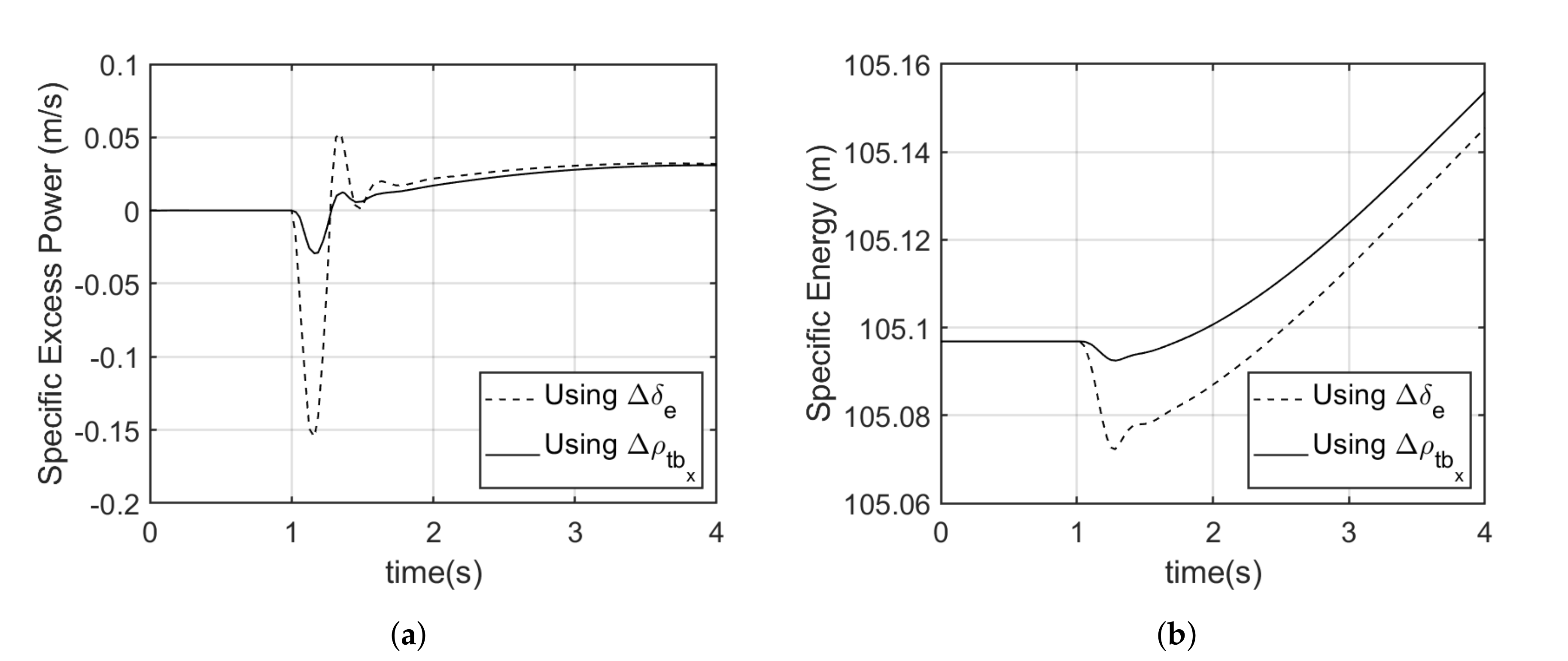
The two alternative moment generation mechanisms were able to achieve the same pull up maneuver as the elevator as shown in Figure 10a and Figure 12a. In the case of the Model 1, an average of 0.9% more specific energy was recorded when using tail displacement in comparison with using the elevator. Looked at across a short time period near the maneuver, the drop in specific excess power using tail movement was around −0.03 m/s, where it was −0.15 m/s using control surface deflection. Over a 4 s window, an average of 1.39% more excess power was recorded when using tail displacement in comparison to using the conventional elevator (see Figure 9).
For the Model 2 aircraft, an average of 1% more specific energy was recorded when using tail angular deflection in comparison with using the elevator. Whereas, an average of 1.83% more excess power was recorded when using tail displacement in comparison with using the conventional elevator (see Figure 11). Again, the transient specific excess power drop was negligible when using tail movement, but around 0.1m/s when using control surface deflection.
Generally, an aircraft that is able to maintain a higher specific energy and excess power has more maneuver advantage [40]. The negative average P s observed when using the elevator to initiate the maneuver results from the drag being greater than available thrust, which results in decreased energy. This is due to the additional drag induced as a result of elevator deflection [33,40].
Although the percentage savings in specific energy states and rates caused by using either of the tail actuation modes as opposed to using the conventional elevator may seem small in magnitude, they make a difference in combat. A dragonfly in pursuit of prey for instance, but particularly in territorial conflict, is engaged in pure aerial combat. In such bouts, dragonflies may be required to make the same or a combination of energy consuming maneuvers in sequence, in a life or death conflict to deplete the opponent’s energy. The transient advantage of using a more energy efficient control effector to initiate a maneuver is substantial by the standards of optimisation of flying systems.
Whilst the results obtained in this study illustrate the potential energy effectiveness demonstrated by insects in flight, fidelity was deliberately limited. The aircraft dynamics model could be made more comprehensive by including the actuator dynamics to quantify the energy required by the actuator to actuate the tail mass when correcting for the imbalance as well as for dynamic maneuvers. Given that the tail was modelled as a point mass and for reduced complexity, its aerodynamic properties were ignored. However, in analysing the stability of the hang-glider where control is achieved by the movement of the pilot relative to the wing, [61] undertook experiments in the wind tunnel to evaluate the aerodynamics on a pilot. Results showed the lift and pitching moment were negligible, and although the drag was significant, its variation with AoA was small. Therefore, future studies should include the aerodynamic effects of actuated abdomens.
Abdominal postures should be explored in high speed footage of dragonflies when capturing prey and across the cycle of feeding and flying, possibly in existing high speed video footage such Georg Rüppell’s contributions that are publicly available at [11].

6. Conclusions

We have mathematically expressed the basic means by which the abdomen of an efficient natural flyer like the dragonfly might be used to save energy and reduce peak power requirements in flight. The abdomen might save energy with reactive responses to achieve longitudinal balance and pull up maneuvers by manipulating moments. Active creation of torques is possible through movement of the abdomen. From analysis of a simulation model of a fixed wing aircraft with an articulated tail structure, we have shown that the amount of energy that might be saved by these techniques can be substantial. We have shown that flight power increases would be required to substitute for the transient effects that can be generated using the movement of the abdomen, while the possibility of trimming balance through tail posture might save energy for as long as the imbalance exists.
In translating these results to technological aircraft, there is a question of overall system integration since an abdomen may not have utility and would thus be simply excess weight. Aircraft may have similar problems to dragonflies in some applications, for example a variable payload weight, a need to fold or fit into a small space, combined with a benefit from high angular accelerations. The dragonfly also reveals that if there is a need to interact with the environment, in the dragonfly case this includes mating and oviposition, a long articulated abdomen is at least as useful as a long nose and intuitively less problematic.

Author Contributions

Conceptualisation, J.C., T.O., methodology, T.O., E.A., N.A.J., execution of study, T.O., J.C., B.M.; writing—original draft preparation, T.O. and J.C.; writing—review and editing, all authors. All authors have read and agreed to the published version of the manuscript.

Funding

This research received no external funding.

Acknowledgments

This work was supported by the Australian Government Research Training Program international (RTPi) scholarship.

Conflicts of Interest

The authors declare no conflict of interest.

Nomenclature

ρ a b Position of point a relative to point b
V A B Velocity of the centre of mass of a rigid body A relative to reference frame B
ω A B Angular velocity of frame A relative to frame B
m A Mass of rigid body A
A Rigid body A
J a A Inertia tensor of rigid body A about its centre of mass at point a
[ X ] A (X (model, vector or tensor) expressed in reference frame A
[ R ] B A The rotation matrix from reference frame A to B
[ R ¯ ] B A Transpose of rotation matrix [ R ] B A
A ˜ Skew symmetric matrix associated with vector A
0 Subscript depicts initial/nominal value
Δ Represents a change from nominal value

References

  1. Dyhr, J.P.; Cowan, N.J.; Colmenares, D.J.; Morgansen, K.A.; Daniel, T.L. Autostabilizing airframe articulation: Animal inspired air vehicle control. In Proceedings of the 2012 IEEE 51st IEEE Conference on Decision and Control (CDC), Hawaii, HI, USA, 10–13 December 2012; pp. 3715–3720. [Google Scholar]
  2. Kohut, N.J. Inertial and Aerodynamic Tail Steering of a Meso-scale Legged Robot; University of California: Berkeley, CA, USA, 2013. [Google Scholar]
  3. Patel, A. Understanding the Motions of the Cheetah Tail Using Robotics. Ph.D. Thesis, University of Cape Town, Cape Town, South Africa, 2015. [Google Scholar]
  4. Camhi, J.M. Yaw-correcting postural changes in locusts. J. Exp. Biol. 1970, 52, 519–531. [Google Scholar]
  5. Camhi, J.M. Sensory control of abdomen posture in flying locusts. J. Exp. Biol. 1970, 52, 533–537. [Google Scholar]
  6. Götz, K.G.; Hengstenberg, B.; Biesinger, R. Optomotor control of wing beat and body posture in Drosophila. Biol. Cybern. 1979, 35, 101–112. [Google Scholar] [CrossRef]
  7. Zanker, J.M. How does lateral abdomen deflection contribute to flight control of Drosophila melanogaster? J. Comp. Physiol. A 1988, 162, 581–588. [Google Scholar] [CrossRef]
  8. Zanker, J. On the mechanism of speed and altitude control in Drosophila melanogaster. Physiol. Entomol. 1988, 13, 351–361. [Google Scholar] [CrossRef]
  9. Luu, T.; Cheung, A.; Ball, D.; Srinivasan, M.V. Honeybee flight: A novel ‘streamlining’response. J. Exp. Biol. 2011, 214, 2215–2225. [Google Scholar] [CrossRef] [PubMed] [Green Version]
  10. Hinterwirth, A.J.; Daniel, T.L. Antennae in the hawkmoth Manduca sexta (Lepidoptera, Sphingidae) mediate abdominal flexion in response to mechanical stimuli. J. Comp. Physiol. 2010, 196, 947–956. [Google Scholar] [CrossRef] [PubMed]
  11. Rüppell, G.; Hilfert-Rüppell, D.; Schneider, B.; Dedenbach, H. On the firing line–interactions between hunting frogs and Odonata. Int. J. Odonatol. 2020, 23, 199–217. [Google Scholar] [CrossRef]
  12. Du, C.; Xu, J.; Zheng, Y. Modeling and control of a dragonfly-like micro aerial vehicle. Adv Robot. Autom. S 2015, 2, 2. [Google Scholar]
  13. Dyhr, J.P.; Morgansen, K.A.; Daniel, T.L.; Cowan, N.J. Flexible strategies for flight control: An active role for the abdomen. J. Exp. Biol. 2013, 216, 1523–1536. [Google Scholar] [CrossRef] [Green Version]
  14. Anderson, J. Aircraft Performance and Design; McGraw-Hill International Editions: Aerospace Science/ Technology Series; WCB/McGraw-Hill: New York, NY, USA, 1999. [Google Scholar]
  15. Koerhuis, C.; Hof, A.; van der Heide, F. Energy consumption in static muscle contraction. Eur. J. Appl. Physiol. 2003, 88, 588–592. [Google Scholar] [CrossRef] [PubMed]
  16. Chahl, J.; Dorrington, G.; Premachandran, S.; Mizutani, A. The dragonfly flight envelope and its application to micro uav research and development. IFAC Proc. Vol. 2013, 46, 231–234. [Google Scholar] [CrossRef]
  17. Marden, J.H. Maximum lift production during takeoff in flying animals. J. Exp. Biol. 1987, 130, 235–258. [Google Scholar]
  18. Olberg, R.M. Visual control of prey-capture flight in dragonflies. Curr. Opin. Neurobiol. 2012, 22, 267–271. [Google Scholar] [CrossRef]
  19. Olberg, R.; Worthington, A.; Venator, K. Prey pursuit and interception in dragonflies. J. Comp. Physiol. A 2000, 186, 155–162. [Google Scholar] [CrossRef]
  20. Combes, S.; Rundle, D.; Iwasaki, J.; Crall, J.D. Linking biomechanics and ecology through predator–prey interactions: Flight performance of dragonflies and their prey. J. Exp. Biol. 2012, 215, 903–913. [Google Scholar] [CrossRef] [Green Version]
  21. Wakeling, J.; Ellington, C.P. Dragonfly flight. I. Gliding flight and steady-state aerodynamic forces. J. Exp. Biol. 1997, 200, 543–556. [Google Scholar] [PubMed]
  22. Azuma, A.; Watanabe, T. Flight performance of a dragonfly. J. Exp. Biol. 1988, 137, 221–252. [Google Scholar]
  23. Newman, B. Model test on a wing section of a dragonfly. Scale Eff. Anim. Locomot. 1977, 445–477. [Google Scholar]
  24. May, M.L. A critical overview of progress in studies of migration of dragonflies (Odonata: Anisoptera), with emphasis on North America. J. Insect Conserv. 2013, 17, 1–15. [Google Scholar] [CrossRef] [Green Version]
  25. Scorer, R. The nature of convection as revealed by soaring birds and dragonflies. Q. J. R. Meteorol. Soc. 1954, 80, 68–77. [Google Scholar] [CrossRef]
  26. Heinrich, B.; Casey, T.M. Heat transfer in dragonflies:‘Fliers’ and ‘perchers’. J. Exp. Biol. 1978, 74, 17–36. [Google Scholar]
  27. Mitchell, F.L.; Lasswell, J.L. Digital Dragonflies. Am. Entomol. 2000, 46, 110–115. [Google Scholar] [CrossRef]
  28. Silsby, J. Dragonflies of the World; CSIRO Publishing: Melbourne, Australia, 2001. [Google Scholar]
  29. Nelson, R.C. Flight Stability and Automatic Control; WCB/McGraw Hill: New York, NY, USA, 1998; Volume 2. [Google Scholar]
  30. Cook, M.V. Flight Dynamics Principles: A Linear Systems Approach to Aircraft Stability and Control; Butterworth-Heinemann: Cambridge, UK, 2012. [Google Scholar]
  31. May, M.L. Thermoregulation and adaptation to temperature in dragonflies (Odonata: Anisoptera). Ecol. Monogr. 1976, 46, 1–32. [Google Scholar] [CrossRef]
  32. May, M. Dependence of flight behavior and heat production on air temperature in the green darner dragonfly Anax junius (Odonata: Aeshnidae). J. Exp. Biol. 1995, 198, 2385–2392. [Google Scholar]
  33. Beard, R.W.; McLain, T.W. Small Unmanned Aircraft: Theory and Practice; Princeton University Press: Princeton, NJ, USA, 2012. [Google Scholar]
  34. Erturk, S.A. Performance Analysis, Dynamic Simulation and Control of Mass-Actuated Airplane. Ph.D. Thesis, University of Texas at Arlington, Arlington, TX, USA, 2016. [Google Scholar]
  35. Waishek, J.; Dogan, A.; Blake, W. Derivation of the dynamics equations of receiver aircraft in aerial refueling. J. Guid. Control. Dyn. 2009, 32, 586–598. [Google Scholar] [CrossRef] [Green Version]
  36. Sakhaei, A. Dynamic Modelling And Predictive Control For Insect-Like Flapping Wing Aerial Micro Robots. Ph.D. Thesis, Ryerson University, Toronto, ON, USA, 2010. [Google Scholar]
  37. Zipfel, P.H. Modeling and Simulation of Aerospace Vehicle Dynamics; American Institute of Aeronautics and Astronautics: Reston, VA, USA, 2007. [Google Scholar]
  38. Nel, A.; Prokop, J.; Pecharová, M.; Engel, M.S.; Garrouste, R. Palaeozoic giant dragonflies were hawker predators. Sci. Rep. 2018, 8, 12141. [Google Scholar] [CrossRef] [PubMed]
  39. Mohammad, H.S. Aircraft Design: A Systems Engineering Approach; John Wiley & Sons: Hoboken, NJ, USA, 2012. [Google Scholar]
  40. Shaw, R.L. Fighter Combat. In Tactics and Maneuvering; Naval Institute Press: Annapolis, MD, USA, 1985. [Google Scholar]
  41. Lambregts, A. Automatic flight control: Concepts and methods. J. FAA Natl. Resour. Spec. Adv. Control. 1995, 2001–2003. [Google Scholar]
  42. Balmer, G.R. Modelling and Control of a Fixed-wing UAV for Landings on Mobile Landing Platforms. Master’s Thesis, Royal Institute of Technology, Stockholm, Sweden, 2015. [Google Scholar]
  43. MATLAB. 9.7.0.1190202 (R2019b); The MathWorks Inc.: Natick, MA, USA, 2019. [Google Scholar]
  44. Okamoto, M.; Yasuda, K.; Azuma, A. Aerodynamic characteristics of the wings and body of a dragonfly. J. Exp. Biol. 1996, 199, 281–294. [Google Scholar]
  45. Chitsaz, N.; Marian, R.; Chahl, J. Experimental method for 3D reconstruction of Odonata wings (methodology and dataset). PloS ONE 2020, 15, e0232193. [Google Scholar] [CrossRef]
  46. Drela, M.; Youngren, H. AVL Overview. 2014. Available online: http://web.mit.edu/drela/Public/web/avl/ (accessed on 12 June 2020).
  47. Drela, M.; Youngren, H. XFOIL Manual. 2001. Available online: http://web.mit.edu/aeroutil_v1.0/xfoil_doc.txt (accessed on 10 June 2020).
  48. Deperrois, A. XFLR5 Analysis of Foils and Wings Operating at Low Reynolds Numbers. 2009. Available online: https://engineering.purdue.edu/~aerodyn/AAE333/FALL10/HOMEWORKS/HW13/XFLR5_v6.01_Beta_Win32%282%29/Release/Guidelines.pdf (accessed on 10 June 2020).
  49. Budziak, K. Aerodynamic Analysis with Athena Vortex Lattice (AVL); Aircraft Design and Systems Group (AERO), Department of Automotive: Hamburg, Germany, 2015. [Google Scholar]
  50. Tsagarakis, M. Project Solaris-Analysis of Airfoil for Solar Powered Flying Wing UAV. Master’s Thesis, Mälardalen University, Västerås, Sweden, 2011. [Google Scholar]
  51. Airfoil Database for Tailless and Flying Wings. Available online: https://www.aerodesign.de/english/profile/profile_s.htm (accessed on 6 April 2020).
  52. Wick, P. Peter Wick on Planks. Part 3: The good slope plank. Radio Control. Soar. Dig. 2006, 23, 7–11. [Google Scholar]
  53. Song, L.; Yang, H.; Zhang, Y.; Zhang, H.; Huang, J. Dihedral influence on lateral–directional dynamic stability on large aspect ratio tailless flying wing aircraft. Chin. J. Aeronaut. 2014, 27, 1149–1155. [Google Scholar] [CrossRef] [Green Version]
  54. Loth, J. Engineering Approach to Aerodynamics and Aircraft Performance; McGraw Hill: New York, NY, USA, 2007. [Google Scholar]
  55. Drela, M.; Youngren, H. AVL 3.36 User Primer. 2017. Available online: http://web.mit.edu/drela/Public/web/avl/avl_doc.txt (accessed on 10 June 2020).
  56. Abzug, M.J.; Larrabee, E.E. Airplane Stability and Control: A History of the Technologies that Made Aviation Possible; Cambridge University Press: Cambridge, UK, 2005; Volume 14. [Google Scholar]
  57. Borri, M.; Trainelli, L. Basic airplane equilibrium and stability revisited. In Proceedings of the International Conference on Aeronautical Science and Air Transportation (ICASAT) Tripoli, Tripoli, Libya, 23–25 April 2007; Volume 23, p. 25. [Google Scholar]
  58. Dantsker, O.D.; Theile, M.; Caccamo, M. A High-Fidelity, Low-Order Propulsion Power Model for Fixed-Wing Electric Unmanned Aircraft. In Proceedings of the 2018 AIAA/IEEE Electric Aircraft Technologies Symposium (EATS), Cincinnati, OH, USA, 12–14 July 2018; pp. 1–16. [Google Scholar]
  59. Ly, J.K. Angle of Attack Determination Using Inertial Navigation System Data from Flight Tests. Ph.D. Thesis, University of Tennessee, Knoxville, TX, USA, 2017. [Google Scholar]
  60. Bomphrey, R.J.; Nakata, T.; Henningsson, P.; Lin, H.T. Flight of the dragonflies and damselflies. Philos. Trans. R. Soc. Biol. Sci. 2016, 371, 20150389. [Google Scholar] [CrossRef] [PubMed] [Green Version]
  61. Kilkenny, E. Full Scale Wind Tunnel Tests on Hang Glider Pilots; College of Aeronautics Report 8416; Cranfield Institute of Technology: Bedford, UK, 1984. [Google Scholar]
Figure 1. Outlines of representative dragonflies from different families. (a) Aeshnidae, Epiaeschna heros. (b) Libellulidae, Libellula croceipennis Selys. (c) Gomphidae, Erpetogomphus designatus Hagen. (d) Petaluridae, Petalura ingentissima; Reprint with permission [27], © 2000, Entomological Society of America.
Energies 13 05480 g001
Figure 2. Dragonfly side view showing longitudinal tail actuation modes. (a) Tail contraction and extension. (b) Tail up down wag movement.
Energies 13 05480 g002
Figure 3. Definition of coordinate systems: Inertial (I), Body (B) and Tail (T).
Energies 13 05480 g003
Figure 4. Forces acting on the aircraft model in flight.
Energies 13 05480 g004
Figure 5. Aircraft model in Simulink.
Energies 13 05480 g005
Figure 6. Phoenix airfoil characteristics. (a) Lift curve. (b) Drag polar.
Energies 13 05480 g006
Figure 7. Aircraft model in AVL.
Energies 13 05480 g007
Figure 8. Model 1 trim in steady level powered flight for a range of airspeed. (a) Elevator deflection. (b) Power required.
Energies 13 05480 g008
Figure 9. Model 2 trim in steady level powered flight for a range of airspeed. (a) Elevator deflection vs. airspeed. (b) Power required vs. airspeed.
Energies 13 05480 g009
Figure 10. Model 1 aircraft pull up maneuver time response. (a) Airspeed. (b) Height.
Energies 13 05480 g010
Figure 11. Model 1 aircraft pull up maneuver time response. (a) Specific excess power. (b) Specific energy.
Energies 13 05480 g011
Figure 12. Model 2 aircraft pull up maneuver time response. (a) Airspeed. (b) Height.
Energies 13 05480 g012
Figure 13. Model 2 aircraft pull up maneuver time response. (a) Specific excess power. (b) Specific energy.
Energies 13 05480 g013
Table 1. Aircraft model physical properties.
ParameterValueParameterValue
m B  (kg)0.325 m T  (kg)0.06
Body length, l B  (m)0.3Max. tail length, l T m a x  (m)0.4
Max. body diameter, d B m a x  (m)0.14Tail diameter, d T  (m)0.05
J x x b B  (kg · m 2 )0.00187 b r e f  (m)1.4
J y y b B  (kg · m 2 )0.01117 c r e f  (m)0.19434
J z z B B  (kg · m 2 )0.00934S (m 2 )0.26865
c g b B  (m)[−0.064; 0; 0.003] A R P  (m)[0.025; 0; 0]
Table 2. Physical constraints of control inputs.
LimitationsUnit
20 δ e 20 deg
30 θ T 30 deg
0.464 ρ t b x 0.664 m
Table 3. Steady level trim flight condition for Models 1 and 2.
Model Type V 0  (m/s) H 0  (m) ρ tb x 0  (m) θ T 0 ( ) θ 0 ( ) δ e 0 ( ) T n 0  (N)
Model 1101000.564-−0.252−1.790.825
Model 2 0−0.252−1.790.825
Table 4. Disturbance mass properties.
ParameterValue
m A  (kg)0.04
x d  (m)−0.05
c g A  (m)[−0.062;0;0.003]
J x x a A  (kg · m 2 )0.00934
J y y a A  (kg · m 2 )0.00188
J z z a A  (kg · m 2 )0.01118
Table 5. Model 1 cases for correction of imbalance.
Model 1 CaseDescriptionIllustration
Case 1Initially balanced with contracted tail,
m = 0.385 kg, ρ t b = 0.564 m.
Energies 13 05480 i001
Case 2Disturbed and unbalanced with contracted tail,
m = 0.425 kg, ρ t b = 0.564 m.
Energies 13 05480 i002
Case 3Disturbed and balanced with extended tail,
m = 0.385 kg, ρ t b = 0.614 m.
Energies 13 05480 i003
Note: Energies 13 05480 i004 represents the added mass.
Table 6. Trimmed steady cruise elevator deflection and power required for Model 1 cases.
Model 1 CaseRange of δ e Range of P req
Case 1−14.5  to −0.0798 4.18 W to 23 W
Case 2−21.2  to −0.763 5.4 W to 24 W
Case 3−17  to −0.309 5.07 W to 23.4 W
Table 7. Model 2 cases for correction of imbalance.
Model 2 CaseDescriptionIllustration
Case 1Initially balanced with deflected tail,
m = 0.385 kg, θ T = 30 .
Energies 13 05480 i005
Case 2Disturbed and unbalanced with deflected tail,
m = 0.425 kg , θ T = 30 .
Energies 13 05480 i006
Case 3Disturbed and balanced with undeflected tail,
m = 0.425 kg, θ T = 0
Energies 13 05480 i007
Note: Energies 13 05480 i008 represents the added mass.
Table 8. Trimmed steady cruise elevator deflection and power required for Model 2 cases.
Model 2 CaseRange of δ e Range of P req
Case 1−6.9  to 0.251 3.57 W to 22.6 W
Case 2−13  to −0.415 4.74 W to 23.5 W
Case 3−12.7  to 0.142 4.71 W to 22.9 W
Table 9. Aircraft Model 1 pull up maneuver control effector comparison using Δ δ e or Δ ρ t b x .
Control Effector UsedAverage Specific Energy (m)Average Specific Excess Power (m/s)
Δ δ e ( ) 105.096−0.007
Δ ρ t b x  (m)105.1050.0069
Table 10. Aircraft Model 2 trim condition before pull up.
V 0  (m/s) H 0  (m) ρ jb x 0  (m) ρ tj x 0  (m) θ T 0 ( ) θ 0 ( ) δ e 0 ( ) T n 0  (N)
101000.2640.4−30−0.66−0.8630.786
Table 11. Aircraft Model 2 pull up maneuver control effector comparison using Δ δ e or Δ θ T .
Control Effector UsedAverage Specific Energy (m)Average Specific Excess Power (m/s)
Δ δ e ( ) 105.093−0.014
Δ θ T ( ) 105.1030.0043
Publisher’s Note: MDPI stays neutral with regard to jurisdictional claims in published maps and institutional affiliations.

