Decomposed Iterative Optimal Power Flow with Automatic Regionalization

Abstract

The optimal power flow (OPF) problem plays an important role in power system operation and control. The problem is nonconvex and NP-hard, hence global optimality is not guaranteed and the complexity grows exponentially with the size of the system. Therefore, centralized optimization techniques are not suitable for large-scale systems and an efficient decomposed implementation of OPF is highly demanded. In this paper, we propose a novel and efficient method to decompose the entire system into multiple sub-systems based on automatic regionalization and acquire the OPF solution across sub-systems via a modified MATPOWER solver. The proposed method is implemented in a modified solver and tested on several IEEE Power System Test Cases. The performance is shown to be more appealing compared with the original solver.

1. Introduction

Optimal power flow (OPF) was first formulated by Carpentier [1], and has since become a crucial task in power system operation and control. The main goal of OPF is to minimize the cost of operation under system constraints. Although many OPF solutions considering different settings have been proposed and there are many commercial products available (see e.g., [2,3]), they are mostly done in a centralized manner, where the loads, generators, transmission lines of a power system covering a large geographical area are all jointly considered. OPF is a non-convex optimization problem, where the non-convexity comes from the nonlinear relationship between voltages and the complex powers demanded or injected at the nodes. Traditional methods for the OPF problem, such as the widely adopted Newton–Raphson solution method, generally return suboptimal load flow solutions of these non-convex problems, and are often computationally complicated. In addition, traditional methods are usually centralized and demonstrate poor scalability. As the power systems are growing in both size and complexity, it will take even longer time and more computational resources for these centralized methods to reach solutions. In summary, there are two major challenges in the existing solutions,

(i)

Optimality: the OPF is non-convex in both its objective function and constraints, and hence finding the global optimum is not guaranteed.

(ii)

Scalability: OPF is an NP-hard problem and the complexity usually grows exponentially with the size of the system. It is quite possible that a proposed solution works well for small systems, but fails to converge to a solution for large systems.

To mitigate these concerns, a decomposed iterative reformulation of the OPF problem for balanced transmission systems was proposed, where the global optimality can be assessed by checking the rank of the obtained voltage-related matrix [4]. Considering that most electrical networks exhibit noticeable sparsity in its bus admittance matrix, it is possible to find a promising decomposition structure. Furthermore, compared with centralized methods, distributed methods are more desirable in terms of security and privacy since they do not require the system to collect and maintain possibly sensitive data or information from one central node [5]. Hence, distributed approaches have great potential for the OPF problem, especially for a large power system.

Over the decades, many heuristic distributed solutions have been proposed. One possible and popular way to address the non-convexity nature of the problem and approach the global optimality is to first convexify the problem via relaxation techniques so that a lower bound of the OPF could be found. Then, this lower bound can be used to evaluate and guide the search for a feasible solution (see e.g., [6,7,8,9,10,11,12,13,14]). However, even with this convex relaxation and the guidance of the lower bound, a good feasible solution is not always available. In addition, solving the relaxed problem introduces an additional computational burden. To address the scalability issue, large-size optimization problems are decomposed into smaller ones. The first distributed method for the OPF problem was studied in [15], where the transmission network is divided into two regions and different decomposition methods are examined to find the solution distributively among these two regions, including the auxiliary problem principle, predictor–corrector proximal multiplier method, and alternating direction method. Nevertheless, the decomposition of the network is restricted to two-region and the boundary variables are not able to be shared among more than two regions. Recent studies on distributed OPF either decompose the original problems implicitly through the solver itself such as the alternating direction method of multipliers (ADMM) or explicitly by dividing the system into many small-size subsystems and conduct the OPF or Security Constrained Optimal Power Flow (SCOPF) in a distributed manner. Compared with the implicit solutions, the explicit ones are more effective and can better exploit the topology and properties of power systems (see e.g., [15,16,17,18,19,20]). However, there are three common issues in existing distributed OPF solutions:

(i)

The decomposition is achieved manually in an ad hoc manner without any guidance. To date, there has been no reported effort to utilize the topology and property of the original system to conduct better regionalization such that the distributed OPF can achieve improved computational efficiency and optimality.

(ii)

Limited interactions among subsystems are involved during the optimization process. The obtained solutions are ad hoc combinations of the optimal solutions for local subsystems, which compromise the optimality for the whole system.

(iii)

Only one decomposition is studied, which means that the optimization is made for the decomposed local parts without a global consideration of the entire system.

In this paper, we propose a novel decomposed iterative solution for OPF with flexibility on the number of subregions and the division of subregions, which provide new insights into power system operation and control. In most existing solutions, the OPF problem is simply formulated as a mathematical optimization problem and then some general optimization techniques are adopted with limited or even no consideration on the nature of power systems. In contrast, our proposed solution explores the very nature of power systems. Specifically, it utilizes the fact that variables in large power systems are loosely coupled and hence only closely related ones need to be clustered into subsystems. Furthermore, the interactions among different subsystems are considered via an extra layer of iterations to search for the optimal solution. Last but not least, multiple decompositions are included in the optimum searching procedure to ensure global optimality. To improve the scalability and the optimality, we design a three-layer iterative optimization framework: the first layer is within small-size subsystems, the second layer is among the subsystems, and the third layer is across different decompositions. In addition to solving OPF problems with improved scalability and optimality, the proposed framework can also be extended to many other problems in power system operation and control where optimizations are involved. Compared with existing distributed OPF solutions in the literature, our proposed framework has the following features:

• Automatic: an automatic regionalization technique is proposed to decompose the original large system into smaller subsystems, which will balance the computational loads of the resultant subsystems and achieve the maximum independence of the variables in different subsystems to accelerate the convergence speed in iterative optimization.
• General: at the first level, many existing OPF problems or general optimization tools can be applied. We first adopt the two most popular OPF tools, one based on the interior-point method (IPM) and the other based upon ADMM.
• Global: the proposed three-layer framework, especially the added third layer of iteration among different decompositions, will greatly increase the extensiveness of the dimensions the algorithm searches and make the optimization results global in view.

The rest of the paper is organized as follows. Section 2 describes the standard OPF formulation and the decomposed OPF formulation. In Section 3, we present the framework of the proposed method with automatic regionalization. Simulation results and analysis are provided in Section 4. Finally, we conclude the paper in Section 5.

The nomenclature of the paper is denoted as follows. For general problem formulation, p is a set of vectors contains the real power provided by all generators, v is a set of vectors contains voltage phasors at all buses, and s is a set of vectors contains all slack variables. $\mathcal{N}$ is a set of buses in the system. $i_k$ is the current injection at bus $k\in \mathcal{N}$. $v_k$ is the voltage at bus $k\in \mathcal{N}$. ${\mathcal{P}}_k+j{\mathcal{Q}}_k\in \mathbb{C}$ is the complex power flow at bus $k\in \mathcal{N}$. Symbols with superscript $X^D$ are power demand-related, i.e., $P_k^D+j{Q}_k^D\in \mathbb{C}$ is the power demand at bus $k\in \mathcal{N}$. Symbols with superscript $X^G$ are power generation related, i.e., $P_k^G+j{Q}_k^G\in \mathbb{C}$ is the power generated by bus $k\in \mathcal{N}$. $Re\left\{x\right\}+jIm\left\{x\right\}$ are real part and imaginary part of the complex number. Symbols in bold capital letter such as $\mathbf{Y}$, $\mathbf{G}$ and $\mathbf{B}$ are matrices and the symbols in bold lowercase letters such as $\mathbf{i}$ and $\mathbf{v}$ are vectors.

2. Problem Statement

OPF is a well-defined classical problem and has been investigated by many researchers since its first introduction (see e.g., [21]),

$$\begin{array}{c}\hfill \underset{\mathit{p},\mathit{v}}{min}f\left(\mathit{p}\right)=f_m\left(\mathit{p}\right)\end{array}$$

(1a)

$$\begin{array}{c}\hfill \mathit{g}(\mathit{p},\mathit{v})=\mathbf{0}\end{array}$$

(1b)

$$\begin{array}{c}\hfill \mathit{h}\left(\mathit{v}\right)\le \mathbf{0},\end{array}$$

(1c)

where $\mathit{p}$ is the vector containing the real power provided by all generators, which can also be treated as the “control variable” in the problem, $\mathit{v}$ is the vector containing voltage phasors at all buses in the system, which can also be treated as the “state variable". It is worth noting that once the state variable $\mathit{v}$ are known, the control variable $\mathit{p}$ can be calculated from the constraint Equation (1b). Equation (1c) is the inequality constraints describing voltage magnitude limits, line current limits, transmission line limits, generator capacity limits and so on.

2.1. Standard OPF Formulation

In this subsection, we present a detailed formulation of problem (1a). We denote $\mathcal{N}=\{1,2,\dots ,N\}$ nodes as the set of buses and $\mathcal{L}\subseteq \mathcal{N}\times \mathcal{N}$ as set of power flow lines between N nodes to represent an electrical network with N nodes. We denote $i_k=Re\left\{i_k\right\}+jIm\left\{i_k\right\}$ as the injection current at bus $k\in \mathcal{N}$ and $v_k=Re\left\{v_k\right\}+jIm\left\{v_k\right\}$ as the voltage at bus $k\in \mathcal{N}$. Let $P_k^D+j{Q}_k^D\in \mathbb{C}$ and $P_k^G+j{Q}_k^G\in \mathbb{C}$ denote the complex power demand and the complex power generated by bus $k\in \mathcal{N}$, respectively. Hence, the complex power ${\mathcal{P}}_k+j{\mathcal{Q}}_k\in \mathbb{C}$ flow into bus k is given as ${\mathcal{P}}_k+j{\mathcal{Q}}_k=(P_k^G+j{Q}_k^G)-(P_k^D+j{Q}_k^D)$. The complex form of current phasor on line $(m,n)\in \mathcal{L}$ is $i_{mn}=Re\left\{i_{mn}\right\}+jIm\left\{i_{mn}\right\}\in \mathbb{C}$ and the complex power transferred from bus m to the rest of the network is ${\mathcal{P}}_{mn}+j{\mathcal{Q}}_{mn}\in \mathbb{C}$. The admittance matrix $\mathbf{Y}\in {\mathbb{C}}^{N\times N}$ of the network is given as

$$\mathbf{Y}=\left\{\begin{array}{cc}{y}_{mm}+\sum _{(m,n)\in \mathcal{L}}{y}_{mn},\hfill & \mathrm{if} m=n,\hfill \\ -y_{mn},\hfill & \mathrm{if} (m,n)\in \mathcal{L},\hfill \\ 0,\hfill & \mathrm{otherwise},\hfill \end{array}\right.$$

(2)

where $y_{mn}=g_{mn}+j{b}_{mn}\in \mathbb{C}$ is the admittance on the transmission line $(m,n)\in \mathcal{L}$, and $y_{mm}=g_{mm}+j{b}_{mm}\in \mathbb{C}$ is the line-to-ground admittance at bus m. We denote $\mathbf{G}\in {\mathbb{R}}^{N\times N}$ and $\mathbf{B}\in {\mathbb{R}}^{N\times N}$ as the real and imaginary parts of $\mathbf{Y}$, respectively. In particular, ${\left[\mathbf{G}\right]}_{mn}=g_{mn}$ and ${\left[\mathbf{B}\right]}_{mn}=b_{mn}$ and $\mathbf{Y}=\mathbf{G}+j\mathbf{B}$. Then, the detailed OPF problem formulation can be expressed as follows (see also [20]),

$$\begin{array}{cccc}\hfill & \min \hfill & \hfill & \sum _{k\in \mathcal{G}}{f}_k^G\left(p_k^G\right)\hfill \end{array}$$

(3a)

$$\begin{array}{cccc}\hfill & \mathrm{s}.\mathrm{t}.\hfill & \hfill & Re\left\{\mathbf{i}\right\}+jIm\left\{\mathbf{i}\right\}=\mathbf{G}Re\left\{\mathbf{v}\right\}-\mathbf{B}Im\left\{\mathbf{v}\right\}+j\left(\mathbf{B}Re\left\{\mathbf{v}\right\}+\mathbf{G}Im\left\{\mathbf{v}\right\}\right),\hfill \end{array}$$

(3b)

$$\begin{array}{cccc}\hfill & \hfill & & {\mathcal{P}}_k+j{\mathcal{Q}}_k=P_k^G-P_k^D+j\left(Q_k^G-Q_k^D\right),\hfill \end{array}$$

(3c)

$$\begin{array}{cccc}\hfill & \hfill & & Re\left\{i_{mn}\right\}+jIm\left\{i_{mn}\right\}=\left({\mathbf{c}}_{mn}+j{\mathbf{d}}_{mn}\right)(Re\left\{v_m\right\},Re\left\{v_n\right\},Im\left\{v_m\right\},Im\left\{v_n\right\}),\hfill \end{array}$$

(3d)

$$\begin{array}{cccc}\hfill & \hfill & & \mathit{p}+j\mathbf{Q}=Re\left\{\mathbf{v}\right\}\circ Re\left\{\mathbf{i}\right\}+Im\left\{\mathbf{v}\right\}\circ Im\left\{\mathbf{i}\right\}+j\left(Im\left\{\mathbf{v}\right\}\circ Re\left\{\mathbf{i}\right\}-Re\left\{\mathbf{v}\right\}\circ Im\left\{\mathbf{i}\right\}\right),\hfill \end{array}$$

(3e)

$$\begin{array}{cccc}\hfill & \hfill & & {\mathcal{P}}_{mn}+j{\mathcal{Q}}_{mn}=Re\left\{v_m{i}_{mn}\right\}+Im\left\{v_m{i}_{mn}\right\}+j(Im\left\{v_m\right\}Re\left\{i_{mn}\right\}-Re\left\{v_m\right\}Im\left\{i_{mn}\right\}),\hfill \end{array}$$

(3f)

$$\begin{array}{cccc}\hfill & \hfill & & P_k^{G_{min}}\le P_k^G\le P_k^{G_{max}},\hfill \end{array}$$

(3g)

$$\begin{array}{cccc}\hfill & \hfill & & Q_k^{G_{min}}\le Q_k^G\le Q_k^{G_{max}},\hfill \end{array}$$

(3h)

$$\begin{array}{cccc}\hfill & \hfill & & {\left(Re\left\{i_{mn}\right\}\right)}^2+{\left(Im\left\{i_{mn}\right\}\right)}^2\le {\left(i_{mn}^{max}\right)}^2,\hfill \end{array}$$

(3i)

$$\begin{array}{cccc}\hfill & \hfill & & {\mathcal{P}}_{mn}^2+{\mathcal{Q}}_{mn}^2\le {\left(s_{mn}^{max}\right)}^2,\hfill \end{array}$$

(3j)

$$\begin{array}{cccc}\hfill & \hfill & & |{\mathcal{P}}_{mn}|\le {\mathcal{P}}_{mn}^{max},\hfill \end{array}$$

(3k)

$$\begin{array}{cccc}\hfill & \hfill & & {\left(v_k^{min}\right)}^2\le {\left(Re\left\{v_k\right\}\right)}^2+{\left(Im\left\{v_k\right\}\right)}^2\le {\left(v_k^{max}\right)}^2,\hfill \\ \hfill & \hfill & & k\in \mathcal{N},(m,n)\in \mathcal{L},\hfill \end{array}$$

(3l)

We denote the cost of generators at bus k as $f_k^G\left(p_k^G\right)$, and the variables are $P_k^G$, $Q_k^G$, $\mathbf{P}$, $\mathbf{Q}$, $Re\left\{\mathbf{i}\right\}$, $Im\left\{\mathbf{i}\right\}$, $Re\left\{\mathbf{v}\right\}$, $Im\left\{\mathbf{v}\right\}$, and $Re\left\{i_{mn}\right\}$, $Im\left\{i_{mn}\right\}$, ${\mathcal{P}}_{mn}$, ${\mathcal{Q}}_{mn}$ for $(m,n)\in \mathcal{L}$. The constraint (3b) is from $\mathbf{i}=\mathbf{Yv}$, the constraint (3c) is from the law of the conservation of power flow, the constraint (3d) is from that $Re\left\{i_{mn}\right\}=Re\left\{y_{mn}(v_m-v_n)\right\}$, the constraint (3e) is from that the complex power is $(\mathbf{v}\circ {\mathbf{i}}^{*})$, and $Im\left\{i_{mn}\right\}=Im\left\{y_{mn}(v_m-v_n)\right\}$ with ${\mathbf{c}}_{mn}=(g_{mn},-g_{mn},b_{mn},-b_{mn})$ and ${\mathbf{d}}_{mn}=(b_{mn},-b_{mn},-g_{mn},g_{mn})$, and constraint (3f) is from that ${\mathcal{P}}_{mn}=Re\left\{v_m{i}_{mn}^{*}\right\}$ and ${\mathcal{Q}}_{mn}=Im\left\{v_m{i}_{mn}^{*}\right\}$. Note that constraints (3b)–(3f) are imposed by Kirchhoff’s laws associated with the physical structure of electrical network. In addition, constraints (3g)–(3l) are the constraints imposed by system operating limits, where the lower bound data ${(·)}^{min}$ and the upper bound data ${(·)}^{max}$ define the feasible intervals of power, current and voltages in the network. Note that if there is no power generation at a bus k then it is not a generator bus, and hence ${\mathcal{P}}_k^G+j{\mathcal{Q}}_k^G=0$. Then these situations can be formulated as follows:

$$P_k^{G_{min}}=P_k^{G_{max}}=Q_k^{G_{min}}=Q_k^{G_{max}}=0,k\in \mathcal{N}\backslash \mathcal{G}.$$

(4)

The constraints (3e), (3f) and (3l) are nonconvex, which render the entire optimization problem (3) nonconvex. The problem is an NP-hard problem and the complexity grows with the size of the system. Thus, it is generally difficult to achieve global optimality using standard method.

2.2. Decomposed OPF Formulation

For simplicity and without loss of generality, we formulate the original problem (1a) with slack variables introduced as a multi-variable single objective optimization problem with both equality and inequality constraints as follows,

$$\begin{array}{c}\hfill \underset{\mathit{p},\mathit{v},\mathit{s}}{min}f(\mathit{p},\mathit{s},{\mathit{s}}_k)=f_m\left(\mathit{p}\right)+f_s\left(\mathit{s}\right)\end{array}$$

(5a)

$$\begin{array}{c}\hfill \mathit{g}(\mathit{p},\mathit{v},\mathit{s})=\mathbf{0}\end{array}$$

(5b)

$$\begin{array}{c}\hfill \mathit{h}(\mathit{v},\mathit{s})\le \mathbf{0}\end{array}$$

(5c)

$$\begin{array}{c}\hfill {\mathit{g}}_k({\mathit{p}}_k,{\mathit{v}}_k,{\mathit{s}}_k)=\mathbf{0}\end{array}$$

(5d)

$$\begin{array}{c}\hfill {\mathit{h}}_k({\mathit{v}}_k,{\mathit{s}}_k)\le \mathbf{0}\end{array}$$

(5e)

where $\mathit{p}$ and $\mathit{v}$ are the same as in problem (1a), and $\mathit{s}$ is the vector containing all slack variables which are introduced to allow imbalance between the input and output power at buses or violation of transmission line limits or generator capacity. It is worth noting that once the state variable $\mathit{v}$ and the slack variable $\mathit{s}$ are known, the control variable $\mathit{p}$ can be calculated from the constraint Equation (5b). The objective function, $f(\mathit{p},\mathit{s},{\mathit{s}}_k)$, is composed of two parts: (1) the generation costs $f_m\left(\mathit{p}\right)$ at the base case; and (2) the penalty for slack variables (i.e., $\mathit{s}\ne \mathbf{0}$) in the base case. Equation (5c) gives the inequality constraints describing voltage magnitude limits, line current limits, transmission line limits, generator capacity limits and so on. 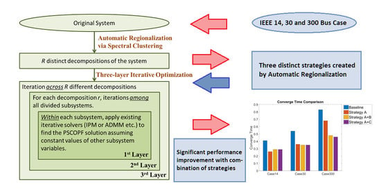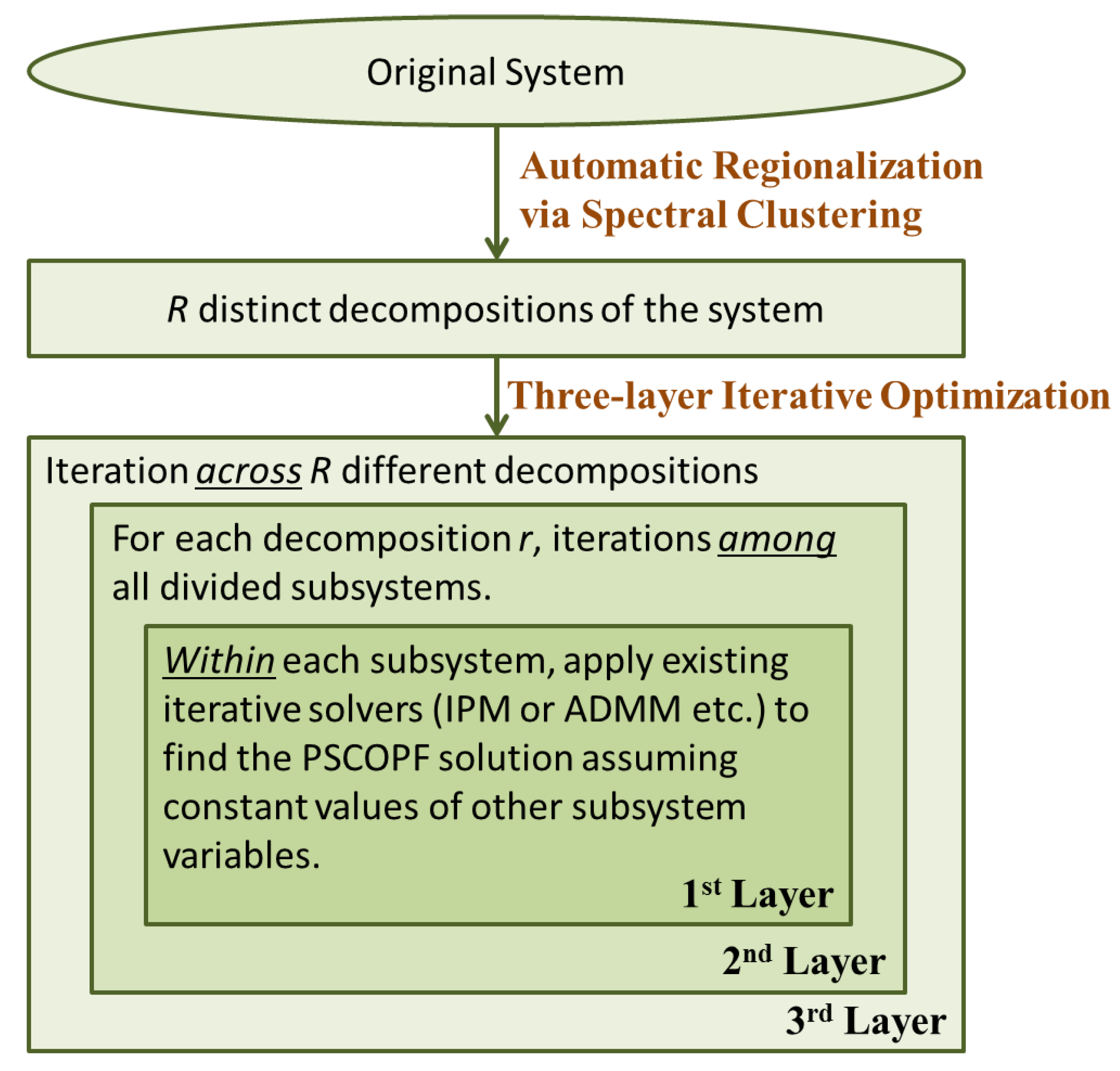Slack variables were also introduced to allow for violations, but penalty was added, which is reflected in $\mathit{s}$ and $f_s\left(\mathit{s}\right)$.The original system was decomposed into several subsystems using the proposed automatic regionalization technique. Notice that several distinct decompositions were provided by the regionalization technique. For a given decomposition, we conducted iterative search among the subsystems. Once it converged and the cost function cannot be further reduced under this decomposition, then we try to work on another decomposition to obtain a better solution. The key is to handle the iterative process at the second layer, which includes the formulation of subsystem optimizations and the iterations among them.

For a given regionalization strategy r with K subsystems in total, we can divide the related variables in the original problem into $\mathit{p}=\left[\begin{array}{c}{\mathit{p}}_{r,1},{\mathit{p}}_{r,2},\dots ,{\mathit{p}}_{r,K}\end{array}\right],\mathit{v}=\left[\begin{array}{c}{\mathit{v}}_{r,1},{\mathit{v}}_{r,2},\dots ,{\mathit{v}}_{r,K}\end{array}\right],\mathit{s}=\left[\begin{array}{c}{\mathit{s}}_{r,1},{\mathit{s}}_{r,2},\dots ,{\mathit{s}}_{r,K}\end{array}\right]$ by reorganizing and combining variables in the same subsystem together. For subsystem k in the i-th iteration, we treat only the variables in that subsystem as unknown and all other variables as known constants using their current values ${\mathit{v}}_{r,k,i}=[{\mathit{v}}_{r,1}^{\left(i\right)},\dots ,{\mathit{v}}_{r,k-1}^{\left(i\right)},{\mathit{v}}_{k,r},{\mathit{v}}_{r,k+1}^{(i-1)},\dots ,{\mathit{v}}_{r,K}^{(i-1)}]$, ${\mathit{s}}_{r,k,i}=[{\mathit{s}}_{r,1}^{\left(i\right)},\dots ,{\mathit{s}}_{r,k-1}^{\left(i\right)},{\mathit{s}}_{k,r},{\mathit{s}}_{r,k+1}^{(i-1)},\dots ,{\mathit{s}}_{r,K}^{(i-1)}]$, ${\mathit{p}}_{r,k,i}=[{\mathit{p}}_{r,1}^{\left(i\right)},\dots ,{\mathit{p}}_{r,k-1}^{\left(i\right)},{\mathit{p}}_{k,r},{\mathit{p}}_{r,k+1}^{(i-1)},\dots ,{\mathit{p}}_{r,K}^{(i-1)}]$.

Then, we plug in those variables into Equations (5a)–(5e) and solve for the optimal solution at the current iteration to obtain ${\mathit{v}}_{k,r}^{\left(i\right)},{\mathit{s}}_{k,r}^{\left(i\right)},{\mathit{v}}_{k,r}^{\left(i\right)}$. Notice that with this formulation: (1) the objective function is unchanged for the entire iteration process; (2) for each iteration, the number of unknown variables is much smaller; and (3) the number of constraint equations is also greatly reduced since most constraints in the original problem will not contain the variables for the subsystem under iteration.

The proposed idea is similar to the many decomposed optimization techniques such as ADMM, conjugate gradient search etc., in the sense that for each iteration, it only searches along a subspace of the unknowns. The difference is that it decomposes the problem by the topology of power systems and utilizes the weak coupling among subsystems. Note from constraint (3b) that the current of each bus is associated with the voltage of itself and its neighboring buses. Hence, constraint (3b) will introduce coupling between adjacent buses. To decouple constraint (3b), we introduce consistency constraints by making each save a copy of each adjacent bus’s voltage and force them to be equal in value.

To formulate the concept above, we denote ${\mathcal{N}}_k$ as the set of bus k itself and its adjacent buses, i.e., ${\mathcal{N}}_k=\left\{k\right\}\cup \left\{n\right|(k,n)\in \mathcal{L}\}$. Copies of real and imaginary parts of the voltages corresponding to buses in ${\mathcal{N}}_k$ is denoted by $Re\left\{{\mathbf{v}}_k\right\}\in {\mathbb{R}}^{|{\mathcal{N}}_k|}$ and $Im\left\{{\mathbf{v}}_k\right\}\in {\mathbb{R}}^{|{\mathcal{N}}_k|}$, respectively. We then denote $Re\left\{\mathbf{v}\right\}$ and $Im\left\{\mathbf{v}\right\}$ as real and imaginary net variables, respectively. The consistency constraints are formulated as follows:

$$Re\left\{{\mathbf{v}}_k\right\}={\mathbf{E}}_{k}Re\left\{\mathbf{v}\right\},Im\left\{{\mathbf{v}}_k\right\}={\mathbf{E}}_{k}Im\left\{\mathbf{v}\right\},$$

(6)

where ${\mathbf{E}}_k\in {\mathbb{R}}^{|{\mathcal{N}}_k|\times N}$ is given by

$${\left({\mathbf{E}}_k\right)}_{mn}=\left\{\begin{array}{cc}1,\hfill & \mathrm{if}{\left(Re\left\{{\mathbf{v}}_k\right\}\right)}_m\mathrm{is}\mathrm{a}\mathrm{local}\mathrm{copy}\mathrm{of}Re\left\{v_n\right\}\hfill \\ 0,\hfill & \mathrm{otherwise}.\hfill \end{array}\right.$$

(7)

Note that (6) is the variable assignment for the net variable copies, for any bus k, either $Re\left\{{\mathbf{v}}_k\right\}$ or $Im\left\{{\mathbf{v}}_k\right\}$ is local and depend only on adjacent buses.

The constraints (3b)–(3l) then can be written by using local variables $Re\left\{{\mathbf{v}}_k\right\}$ and $Im\left\{{\mathbf{v}}_k\right\}$. Accordingly, we can list them as follows,

$$\begin{array}{cc}\hfill & Re\left\{i_k\right\}+jIm\left\{i_k\right\}={\mathbf{g}}_k^{T}Re\left\{{\mathbf{v}}_k\right\}-{\mathbf{b}}_k^{T}Im\left\{{\mathbf{v}}_k\right\}+j\left({\mathbf{b}}_k^{T}Re\left\{{\mathbf{v}}_k\right\}+{\mathbf{g}}_k^{T}Im\left\{{\mathbf{v}}_k\right\}\right),\hfill \end{array}$$

(8a)

$$\begin{array}{cc}\hfill & {\mathcal{P}}_k+j{\mathcal{Q}}_k=P_k^G-P_k^D+j\left(Q_k^G-Q_k^D\right),\hfill \end{array}$$

(8b)

$$\begin{array}{cc}\hfill & Re\left\{{\overline{\mathbf{i}}}_k\right\}+jIm\left\{{\overline{\mathbf{i}}}_k\right\}={\mathbf{C}}_{k}Re\left\{{\mathbf{v}}_k\right\}+{\mathbf{D}}_{k}Im\left\{{\mathbf{v}}_k\right\}+j\left({\mathbf{D}}_{k}Re\left\{{\mathbf{v}}_k\right\}-{\mathbf{C}}_k{\mathbf{v}}_k^{Im}\right),\hfill \end{array}$$

(8c)

$$\begin{array}{cc}\hfill & {\mathcal{P}}_k+j{\mathcal{Q}}_k={\left(Re\left\{{\mathbf{v}}_k\right\}\right)}_{1}Re\left\{i_k\right\}+{\left(Im\left\{{\mathbf{v}}_k\right\}\right)}_{1}Im\left\{i_k\right\}+j\left({\left(Im\left\{{\mathbf{v}}_k\right\}\right)}_{1}Re\left\{i_k\right\}-{\left(Re\left\{{\mathbf{v}}_k\right\}\right)}_{1}Im\left\{i_k\right\}\right),\hfill \end{array}$$

(8d)

$$\begin{array}{cc}\hfill & {\overline{\mathbf{P}}}_k+j{\overline{\mathbf{Q}}}_k={\left(Re\left\{{\mathbf{v}}_k\right\}\right)}_{1}Re\left\{{\overline{\mathbf{i}}}_k\right\}+{\left(Im\left\{{\mathbf{v}}_k\right\}\right)}_{1}Re\left\{{\overline{\mathbf{i}}}_k\right\}+j\left({\left(Im\left\{{\mathbf{v}}_k\right\}\right)}_{1}Re\left\{{\mathbf{i}}_k\right\}-{\left(Re\left\{{\mathbf{v}}_k\right\}\right)}_{1}Im\left\{{\mathbf{i}}_k\right\}\right),\hfill \end{array}$$

(8e)

$$\begin{array}{cc}\hfill & P_k^{G_{min}}\le P_k^G\le P_k^{G_{max}},\hfill \end{array}$$

(8f)

$$\begin{array}{cc}\hfill & Q_k^{G_{min}}\le Q_k^G\le Q_k^{G_{max}},\hfill \end{array}$$

(8g)

$$\begin{array}{cc}\hfill & {\left(Re\left\{{\overline{\mathbf{i}}}_k\right\}\right)}_r^2+{\left(Im\left\{{\overline{\mathbf{i}}}_k\right\}\right)}_r^2\le {\left({\overline{\mathbf{i}}}_k^{max}\right)}_r^2,r=1,\dots ,\left|{\mathcal{N}}_k\right|-1,\hfill \end{array}$$

(8h)

$$\begin{array}{cc}\hfill & {\left({\overline{\mathbf{P}}}_k\right)}_r^2+{\left({\overline{\mathbf{Q}}}_k\right)}_r^2\le {\left({\mathbf{s}}_k^{max}\right)}_r^2,r=1,\dots ,\left|{\mathcal{N}}_k\right|-1,\hfill \end{array}$$

(8i)

$$\begin{array}{cc}\hfill & |{\left({\overline{\mathbf{P}}}_k\right)}_r|\le {\left({\overline{\mathbf{P}}}_k^{max}\right)}_r,r=1,\dots ,\left|{\mathcal{N}}_k\right|-1,\hfill \end{array}$$

(8j)

$$\begin{array}{cc}\hfill & {\left({\mathbf{v}}_k^{min}\right)}_r^2\le {\left(Re\left\{{\mathbf{v}}_k\right\}\right)}_r^2+{\left(Im\left\{{\mathbf{v}}_k\right\}\right)}_r^2\le {\left({\mathbf{v}}_k^{max}\right)}_r^2,r=1,\dots ,\left|\mathcal{N}\right|,\hfill \end{array}$$

(8k)

where $Re\left\{{\overline{\mathbf{i}}}_k\right\}={\left(Re\left\{i_{kl}\right\}\right)}_{l\in {\mathcal{N}}_k\backslash \left\{k\right\}}$, $Im\left\{{\overline{\mathbf{i}}}_k\right\}={\left(Im\left\{i_{kl}\right\}\right)}_{l\in {\mathcal{N}}_k\backslash \left\{k\right\}}$, ${\overline{\mathbf{P}}}_k={\left(p_{kl}\right)}_{l\in {\mathcal{N}}_k\backslash \left\{k\right\}}$, and ${\overline{\mathbf{Q}}}_k={\left(q_{kl}\right)}_{l\in {\mathcal{N}}_k\backslash \left\{k\right\}}$, where $k\in \mathcal{N}$, with the same order as in ${\left(Re\left\{{\mathbf{v}}_k\right\}\right)}_{1:|{\mathcal{N}}_k|}$ and ${\left(Im\left\{{\mathbf{v}}_k\right\}\right)}_{1:|{\mathcal{N}}_k|}$. In addition, ${\mathbf{g}}_k$ (or ${\mathbf{b}}_k$) in constraint (8a) are acquired from the k-th column of $\mathbf{G}$ (respectively, $\mathbf{B}$) and then extracting the rows corresponding to the buses in ${\mathcal{N}}_k$ with the same order as in $Re\left\{{\mathbf{v}}_k\right\}$ and $Im\left\{{\mathbf{v}}_k\right\}$. Accordingly, ${\mathbf{C}}_k\in {\mathbb{R}}^{\left(\right|{\mathcal{N}}_k|-1)\times |{\mathcal{N}}_k|}$ and ${\mathbf{D}}_k\in {\mathbb{R}}^{\left(\right|{\mathcal{N}}_k|-1)\times |{\mathcal{N}}_k|}$ in constraint (8c) are constructed as follows

$$\begin{array}{cc}\hfill {\mathbf{C}}_k& =\left(\begin{array}{cccc}{\left({\mathbf{g}}_k\right)}_2& -{\left({\mathbf{g}}_k\right)}_2& \cdots & 0\\ {\left({\mathbf{g}}_k\right)}_3& 0& \cdots & 0\\ ⋮& ⋮& \ddots & ⋮\\ {\left({\mathbf{g}}_k\right)}_{|{\mathcal{N}}_k|-1}& 0& \cdots & -{\left({\mathbf{g}}_k\right)}_{|{\mathcal{N}}_k|}\end{array}\right),\mathrm{and}\hfill \end{array}$$

(9)

$$\begin{array}{cc}\hfill {\mathbf{D}}_k& =\left(\begin{array}{cccc}{\left({\mathbf{b}}_k\right)}_2& -{\left({\mathbf{b}}_k\right)}_2& \cdots & 0\\ {\left({\mathbf{b}}_k\right)}_3& 0& \cdots & 0\\ ⋮& ⋮& \ddots & ⋮\\ {\left({\mathbf{b}}_k\right)}_{|{\mathcal{N}}_k|-1}& 0& \cdots & -{\left({\mathbf{b}}_k\right)}_{|{\mathcal{N}}_k|}\end{array}\right).\hfill \end{array}$$

(10)

We substitue constraints (8a)–(8c) as ${\alpha }_k\left({\mathbf{z}}_k\right)=0$, the nonlinear equality constraint (8d) as ${\lambda }_k\left({\mathbf{z}}_k\right)=0$, the nonlinear equality constraint (8e) as ${\mu }_k\left({\mathbf{z}}_k\right)=0,$ the linear convex inequality constraints (8f), (8g) and (8j) as ${\beta }_k\left({\mathbf{z}}_k\right)\le 0$, and the nonlinear convex inequality constraints (8h) and (8i) as ${\gamma }_k\left({\mathbf{z}}_k\right)\le 0$. Then, we can rewrite the decomposed formulation of problem (3) as follows,

$$\begin{array}{cccc}\hfill & \min \hfill & \hfill & \sum _{k\in \mathcal{G}}{f}_k^G\left(p_k^G\right)\hfill \end{array}$$

(11a)

$$\begin{array}{cccc}\hfill & \mathrm{s}.\mathrm{t}.\hfill & \hfill & {\mathbf{z}}_k=(P_k^G,Q_k^G,P_k,Q_k,Re\left\{i_k\right\},Im\left\{i_k\right\},Re\left\{{\mathbf{x}}_k\right\},Im\left\{{\mathbf{x}}_k\right\},Re\left\{{\overline{\mathbf{i}}}_k\right\},Im\left\{{\overline{\mathbf{i}}}_k\right\},{\overline{\mathbf{P}}}_k,{\overline{\mathbf{Q}}}_k),k\in \mathcal{N},\hfill \end{array}$$

(11b)

$$\begin{array}{cccc}\hfill & \hfill & & \left({\alpha }_k\left({\mathbf{z}}_k\right),{\lambda }_k\left({\mathbf{z}}_k\right),{\mu }_k\left({\mathbf{z}}_k\right)\right)=0,k\in \mathcal{N},\hfill \end{array}$$

(11c)

$$\begin{array}{cccc}\hfill & \hfill & & \left({\beta }_k\left({\mathbf{z}}_k\right),{\gamma }_k\left({\mathbf{z}}_k\right)\right)\le 0,k\in \mathcal{N},\hfill \end{array}$$

(11d)

$$\begin{array}{cccc}\hfill & \hfill & & {\left({\mathbf{v}}_k^{min}\right)}_r^2\le {\left(Re\left\{{\mathbf{v}}_k\right\}\right)}_r^2+{\left(Im\left\{{\mathbf{v}}_k\right\}\right)}_r^2\le {\left({\mathbf{v}}_k^{max}\right)}_r^2,r=1,\dots ,\left|{\mathcal{N}}_k\right|,k\in \mathcal{N},\hfill \end{array}$$

(11e)

$$\begin{array}{cccc}\hfill & \hfill & & Re\left\{{\mathbf{v}}_k\right\}+jIm\left\{{\mathbf{v}}_k\right\}={\mathbf{E}}_{k}Re\left\{\mathbf{v}\right\}+j{\mathbf{E}}_{k}Im\left\{\mathbf{v}\right\},k\in \mathcal{N}\hfill \end{array}$$

(11f)

where the variables are $P_k^G$, $Q_k^G$, $P_k$, $Q_k$, $Re\left\{i_k\right\}$, $Im\left\{i_k\right\}$, $Re\left\{{\mathbf{v}}_k\right\}$, $Im\left\{{\mathbf{v}}_k\right\}$, $Re\left\{{\overline{\mathbf{i}}}_k\right\}$, $Im\left\{{\overline{\mathbf{i}}}_k\right\}$, ${\overline{\mathbf{P}}}_k$, ${\overline{\mathbf{Q}}}_k$, ${\mathbf{z}}_k$ for $k\in \mathcal{N}$ and $Re\left\{\mathbf{v}\right\}$ and $Im\left\{\mathbf{v}\right\}$. Note that (11f) gives the constructed consistency constraints, which define the consistency voltages among adjacent buses. The coupling in the original centralized formulation (3) has been guaranteed in the consistency constraint (11f) so that decomposition methods can be applied without changing the global objective function.

3. Automatic Regionalization Based OPF (AR-OPF)

In our approach, we aim to address the scalability and the optimality issues of OPF using a systematic decomposed iterative method with automatic regionalization. Specifically, as compared with existing distributed OPF solutions, instead of using only one decomposition of the system, we acquire distinct decompositions of the original system as multiple regionalization strategies based on automatic regionalization via spectral clustering proposed in our previous work [22]. In addition, compared with existing distributed OPF solutions which usually conduct local optimization within each subsystem, but involve few interactions among different subsystems, we introduce two additional layers of iterations to search for the optimal solution: (i) for a single strategy, based on multiple regionalization strategies, we iteratively search for better OPF solutions across different subsystems; (ii) for multiple strategies, combinations of strategies will be created based on previously obtained optimization results and time consumption for convergence, then we iteratively search for better OPF solutions via the combination of different regionalization strategies in addition to optimization within each subsystem. The strategy change will be performed after the previously-used strategy converges under a specified convergence criterion. The added layers of iterations make our optimization to search local optima yet with the global optimality in view. Accordingly, instead of manual and ad hoc decomposition, based upon the considerations of computational loads and the dependencies among different subsystems, we propose an automatic regionalization algorithm to decompose the original large-size system. The proposed algorithm can provide multiple decompositions of a given system, which can then be used for the iterations across decompositions. With the proposed automatic regionalization technique, the system is first decomposed into several subsystems and as a result, the scalability issue can be better addressed. Meanwhile, the iterative procedure is designed in a manner that guarantees a better solution at each iteration. Furthermore, the three-layer iterations can help avoid local optimum and better approach the global optimum.

3.1. Overview of the Algorithm

The framework of the proposed algorithm is shown in Figure 1. First, we conduct automatic regionalization using spectral clustering to decompose the original system into subsystems. There are multiple decompositions with distinct regionalization strategies resulting from our proposed technique. Then, a three-layer iterative optimization procedure will be conducted to find the solution for OPF, where each iteration at any layer is designed in a manner that guarantees a better solution in terms of the global performance. The first layer is within each subsystem, which is an optimization problem with a much smaller number of variables and constraints. The second layer is among the different subsystems. In other words, we alternate among different subsystems to find a better solution for the global OPF problem. The third layer is across different decompositions. At this layer, once a solution is found under a given decomposition, a new regionalization strategy will be used to obtain a different decomposition of the system. Then, the previous solution will be used as the initialization for this new decomposed problem to conduct further 1st- and 2nd-layer iterative optimizations to improve the overall optimality. This provides a global view in our optimization process, even though each iteration is conducted in a local manner.

3.2. Automatic Regionalization via Spectral Clustering

The goal of the regionalization is to decompose the original system into subsystems based on the graph of buses. We propose an automatic regionalization technique based upon two main considerations: (1) we want to distribute the computational load evenly among the subsystems; (2) we want to achieve less inter-region dependence, where the variables among different regions will be affected by other regions in a minimum way. These two considerations will provide faster convergence of the iterative procedure. Accordingly, we propose the k-means spectral clustering technique for automatic regionalization.

Spectral clustering makes use of spectrum of the similarity matrix to cluster the data points, also know as a clustering technique based on the similarity graph of data points. In our case, we define the buses among power system as the data points. Let $G=(V,E)$ be the undirected similarity graph, where $V=\{v_1,\cdots ,v_N\}$ is a vertex set, and each vertex represents a bus. We define the similarity between two buses by non-negative weight $w_{ij}$ of the edge $(i,j)\in E$ according to the topology of the system. Then we denote the weighted adjacency matrix of the graph G as $\mathbf{W}={\left(w_{ij}\right)}_{i,j=1,\cdots ,N}$. The degree of vertex is $d_i={\sum }_{j=1}^N{w}_{ij}$ corresponding to $v_i\in V$ and the degree matrix $\mathbf{D}$ is the diagonal matrix with $d_1,\cdots ,d_N$ on the diagonal. Therefore, we can have the graph Laplacian matrix as $\mathbf{L}=\mathbf{D}-\mathbf{W}$. Technically, we utilize the normalized spectral clustering proposed in [23]. Assuming ${\lambda }_1,\cdots ,{\lambda }_k$ be the smallest eigenvalues of the generalized eigenproblem $\mathbf{L}\mathbf{u}=\lambda \mathbf{D}\mathbf{u}$ where ${\mathbf{u}}_1,\cdots ,{\mathbf{u}}_k$ be the corresponding eigenvectors. Let $\mathbf{U}=[{\mathbf{u}}_1,\cdots ,{\mathbf{u}}_k]$ be a $N\times k$ matrix. Then, let ${\mathbf{y}}_i\in {\mathbb{R}}^k$ denote ith row from matrix $\mathbf{U}$, and with the implementation of k-means algorithm, ${\mathbf{y}}_i=\{{\mathbf{y}}_1,\cdots ,{\mathbf{y}}_N\}$ are clustered into k clusters. At last, the spectral clustering result of the corresponding vertex $v_i$ is obtained from the clustering result ${\mathbf{y}}_i$.

In addition, to guarantee a similar computational burden for each region among subsystems, the number of buses of each subsystem is required to be similar. Hence, we initialize the k-means clustering algorithm by selecting the initial centroids evenly distributed in the sample space at each location. In addition, with different initializations of k-means clustering, different regionalization strategies can be obtained through the proposed automatic regionalization technique.

The similarity graph plays an important role in realizing a regionalization with minimum interactions among different regions. In fact, buses with stronger mutual impact based on the states of the bus tend to be clustered into the same region in spectral clustering. Therefore, it would be reasonable to define the similarity between two buses that can describe the mutual impact. Thus, we construct three types of similarity graphs based on different similarities.

(1)

Topology Based Similarity (TBS): The simplest method is utilizing the topology of the system directly to define the similarity which results in creating a weighted adjacency matrix with 1 s representing a transmission line connects the buses and 0s for otherwise.

(2)

Measurement-Based Similarity (MBS): The states of a bus can only affect its neighbors during operation, which means that there is an available measurement that both buses are involved simultaneously. More specifically, the similarity considers whether there is at least one power flow measurement available on a transmission line, or one power injection measurement available at either one of the buses connected to the line.

(3)

Weighted Measurement-Based Similarity (WMBS): In fact, no two of the buses have the same amount of measurements involved, and not all measurements have the same amount of effect in coupling those involved buses. Under certain circumstances, it will be more favorable to cluster two strongly coupled buses into one region and divide two weakly coupled buses into different regions. Therefore WMBS is considering not only the availability of the measurements, but also the amount and impact of the measurements.

Table 1. Regionalization schemes.

Regionalization	Region 1	Region 2	Region 3	Region 4
Manual Case 1	1, 2, 5	3, 4, 7, 8, 9	10, 11, 14	6, 12, 13
Manual Case 2	1, 2, 5	3, 4, 7, 8	9, 10, 14	6, 11, 12, 13
TBS-AR (A)	1, 2, 3, 4, 5	7, 8, 9	10, 11	6, 12, 13, 14
MBS-AR (B)	1, 2,3,5	4, 7, 8, 9	10, 11	6, 12, 13, 14
WMBS-AR (C)	1, 2, 3, 5	4, 7, 8, 9, 14	10, 11	6, 12, 13

shows the two manual regionalization strategies, as well as the results of the three automatic regionalization strategies achieved by the proposed AR technique.

3.3. Cross-Subsystem Variable Update

In this section, we introduce the overview of the subsystem variables update, then show the cross-subsystem update based on combination of different strategies. The optimization results will be global in view by using variables updated from one subsystem as the newer constant values of another subsystem.

3.3.1. Subsystem Variable Update

Particularized to our problem (11), The partial augmented Lagrangian with respect to the consistency constraints (11f) (i.e., ${\mathbf{v}}_k={\overline{E}}_k\mathbf{v}$) is given by

$$\begin{array}{c}\hfill L_{\rho }({\mathbf{P}}^G,{\left({\mathbf{v}}_k\right)}_{k\in \mathcal{N}},\mathbf{v},{\left({\mathbf{Y}}_k\right)}_{k\in \mathcal{N}})=\sum _{k\in \mathcal{G}}{f}_k^G\left(p_k^G\right)\\ \hfill +\sum _{k\in \mathcal{N}}\left({\mathbf{Y}}_k^T({\mathbf{v}}_k-{\overline{E}}_k\mathbf{v})+\frac{\rho }{2}\left|\right|{\mathbf{v}}_k-{\overline{E}}_k\mathbf{v}{\left|\right|}_2^2\right),\end{array}$$

(12)

where ${\mathbf{Y}}_k$ is dual variable-associated with (11f) and $\rho$ is called the penalty parameter. Together with the separability of (12) among $k\in \mathcal{N}$, steps of the algorithm is presented in Algorithm 1. The first step is the initialization of the algorithms which defines the net and dual variables. Then, next step is to solve a non-convex optimization problem (13) to update the private value of buses k. The following step is to update an unconstrainted quadratic optimization problem (14). After the net variable $\mathbf{v}$ is updated, the dual variable ${\mathbf{y}}_k$ is updated in the next step (15). The last step is the stopping criterion check.

Algorithm 1: Decomposed OPF.

1   Initialization: Set $n=0$ and initialize ${\mathbf{y}}_k^{\left(n\right)}$ and ${\mathbf{v}}^{\left(n\right)}$

2   Private variable update: Set ${\mathbf{y}}_k={\mathbf{y}}_k^{\left(n\right)}$ and $\mathbf{v}={\mathbf{v}}^{\left(n\right)}$. Each bus $k\in \mathcal{N}$ updates ${\mathbf{x}}_k$ locally, where we let $({\mathbf{z}}_k^{(n+1)},{\mathbf{u}}_k^{(n+1)})$ be the primal and dual (possibly) optimal variables achieved for the following problem: $$\begin{array}{cccc}\hfill & \min \hfill & \hfill & f_k^G\left(p_k^G\right)+{\mathbf{y}}_k^T({\mathbf{v}}_k-{\overline{\mathbf{E}}}_k\mathbf{v})+\frac{\rho }{2}\left|\right|{\mathbf{v}}_k-{\overline{\mathbf{E}}}_k\mathbf{v}{\left|\right|}_2^2,\hfill \\ \hfill & \mathrm{s}.\mathrm{t}.\hfill & \hfill & {\mathbf{z}}_k=(P_k^G,Q_k^G,P_k,Q_k,Re\left\{i_k\right\},Im\left\{i_k\right\},Re\left\{{\mathbf{v}}_k\right\},Im\left\{{\mathbf{v}}_k\right\},Re\left\{{\overline{\mathbf{i}}}_k\right\},Im\left\{{\overline{\mathbf{i}}}_k\right\},{\overline{\mathbf{P}}}_k,{\overline{\mathbf{Q}}}_k)\hfill \\ \hfill & \hfill & & {\alpha }_k\left({\mathbf{z}}_k\right)=\mathbf{0}\hfill \\ \hfill & \hfill & & {\lambda }_k\left({\mathbf{z}}_k\right)=\mathbf{0}\hfill \\ \hfill & \hfill & & {\mu }_k\left({\mathbf{z}}_k\right)=\mathbf{0}\hfill & \hfill & \\ \hfill & \hfill & & {\beta }_k\left({\mathbf{z}}_k\right)\le \mathbf{0}\hfill & \hfill & \\ \hfill & \hfill & & {\gamma }_k\left({\mathbf{z}}_k\right)\le \mathbf{0}\hfill & \hfill & \\ \hfill & \hfill & & {\left({\mathbf{v}}_k^{min}\right)}_r^2\le {\left(Re\left\{{\mathbf{v}}_k\right\}\right)}_r^2+{\left(Im\left\{{\mathbf{v}}_k\right\}\right)}_r^2\le {\left({\mathbf{v}}_k^{max}\right)}_r^2,\hfill \\ \hfill & \hfill & & r=1,\dots ,|{\mathcal{N}}_k|,\hfill \end{array}$$ (13) where the variables are $P_k^G$, $Q_k^G$, $P_k$, $Q_k$, $Re\left\{i_k\right\}$, $Im\left\{i_k\right\}$, $Re\left\{{\mathbf{v}}_k\right\}$, $Im\left\{{\mathbf{v}}_k\right\}$, $Re\left\{{\overline{\mathbf{i}}}_k\right\}$, $Im\left\{{\overline{\mathbf{i}}}_k\right\}$, ${\overline{\mathbf{P}}}_k$, ${\overline{\mathbf{Q}}}_k$, and ${\mathbf{z}}_k$. We denote the part of ${\mathbf{z}}_k^{(n+1)}$ corresponding to $(Re\left\{{\mathbf{v}}_k\right\},Im\left\{{\mathbf{v}}_k\right\})$ by ${\mathbf{v}}_k^{(n+1)}$.

3   Net variable update: We denote ${\mathbf{v}}^{(n+1)}$ as the solution to the problem minimize $$min\sum _{k\in \mathcal{N}}{\mathbf{y}}_k^T({\mathbf{v}}_k^{(n+1)}-{\overline{\mathbf{E}}}_k\mathbf{v})+\frac{\rho }{2}\left|\right|{\mathbf{v}}_k^{(n+1)}-{\overline{\mathbf{E}}}_k\mathbf{v}{\left|\right|}_2^2$$ (14) where the variable is $\mathbf{v}$

4   Dual variable update: Each bus $k\in \mathcal{N}$ updates its dual variable ${\mathbf{y}}_k$ as $${\mathbf{y}}_k^{(n+1)}={\mathbf{y}}_k^{\left(n\right)}+\rho ({\mathbf{v}}_k^{(n+1)}-{\overline{\mathbf{E}}}_k{\mathbf{v}}^{(n+1)}).$$ (15)

5   Stopping criterion check: set $n:=n+1$. If the stopping criterion is not reached, go to step 2, otherwise stop and return $\left({\mathbf{z}}^{\left(n\right)},{\mathbf{v}}^{\left(n\right)},{\mathbf{u}}^{\left(n\right)},{\mathbf{y}}^{\left(n\right)}\right)=\left({\left({\mathbf{z}}_k^{\left(n\right)}\right)}_{k\in \mathcal{N}},{\mathbf{v}}^{\left(n\right)},{\left({\mathbf{u}}_k^{\left(n\right)}\right)}_{k\in \mathcal{N}},{\left({\mathbf{y}}_k^{\left(n\right)}\right)}_{k\in \mathcal{N}}\right)$.

3.3.2. Cross-Subsystem

We implement the proposed algorithms to different case with single strategy implemented and after some test run, it can be observed that the number of iterations is increased significantly as expected. In spite of that, there is a possibility of improvement. According to standard OPF, when using a start value close to optimal, the optimization process will convergence faster. Hence, we can improve the performance of the optimization process by using a better and closer start value achieved by a given policy.

We define the stopping criterion as the constraint violation tolerance. To further expand the algorithms to achieve the expected performance improvement, we change the stopping criterion (i.e., the constraint violation tolerance) to stop the optimization process earlier in order to perform a change of regionalization strategy. The optimization process will stop upon reaching a specified target constraint violation tolerance, which is set to be $5\times {10}^{-3}$ in our implementations. Then, the previously used regionalization strategy will be switched to another in the queue from the given strategy combination. The algorithm will then continue running after the different regionalization strategy is updated and the constraint violation tolerance is updated to $5\times {10}^{-6}$. Subsystem variable update will also be applied during optimization. The only thing needed after restarting the process is to alter the label of inputs, power equations and constraints according to the new strategy obtained from the automatic regionalization process.

4. Simulation and Results

In this section, we present the implementation of simulations to our proposed decomposed method and compare the results with centralized OPF using the solver provided by MATPOWER [24,25,26]. To begin with the simulation setup, according to the MATPOWER User’s Manual [27], we applied MATPOWER Interior Point Solver (MIPS) [24] as our primary OPF solver. We firstly verify our approach with different sample cases from IEEE Power System Test Case under a single strategy, then under a combination of strategies. All results were generated by MATLAB 2017b [28] on the same desktop computer with Intel Core i7-6700K Processor@4.00Ghz and 32 GB memory. Test cases of systems with a size of $\mathcal{N}=14,30,300$ were chosen, with non-zero duality gap, in order to study the convergence properties of the decomposed method we proposed. To test the scalability of our approach, we evaluated it on a relatively larger example, such as the IEEE 300-bus system. For different regionalization strategy selection, we changed the stopping criterion in motion in MATPOWER [26] to stop the first round of the optimization process. Then, our optimization process changed from the first regionalization strategy to another one, i.e., the algorithm continues the optimization process subsequently by utilizing a different regionalization policy selected from strategy combined with an updated constraint violation tolerance. Subsystem variable update was applied appropriately in the process of the second-round optimization. We used the regionalization strategies generated by AR and denote TBS-AR as strategy A, MBS-AR as B and WMBS-AR as C. An example of the regionalization on IEEE 14-bus system is shown in Table 1, and bus symbols represented in network topology are given in Figure 2.

4.1. Simulation Result Analysis

In this subsection, we will focus on the result analysis to provide insights towards practical application. Firstly, we ran strategies separately as test runs to figure out which strategy will be applied as the first strategy in the strategy combination. For the 14-bus system, with a default setting that constrains violation tolerance was set to $5\times {10}^{-6}$, both the number of iterations and the convergence time were relatively close, as shown in Figure 3. Then we change the constraint violation tolerance to $5\times {10}^{-3}$, as shown in Figure 4, and find that both the number of iterations and the convergence time of strategy A were slightly better. Detailed optimization results are shown in

Table 2. Single strategy time cost and optimization results.

Results	Original	Strategy A	Strategy B	Strategy C
Converge Time (s)	0.41	0.26	0.29	0.27
Iteration numbers	12	54	60	56
Objfcn Value ($/h)	8081.53	8081.53	8081.53	8081.53
Total Gen P (MW)	268.29	268.29	268.29	268.29
Total Gen Q (MVar)	67.63	67.63	67.63	67.63
Branch Loss P (MW)	9.287	9.287	9.287	9.287
Branch Loss Q (MVar)	39.16	39.16	39.16	39.16

. We are not presenting the results of 30- and 300-bus systems since they behaved similarly. Note that the difference of the convergence time between single strategy was relatively small but for the 300-bus system, there was a big difference between the single strategy and the combination of strategies, as will be shown later. Then, we implemented the combination of two strategies to our proposed AROPF. Apparently, the optimization results obtained by various strategy combinations are different, as shown in Figure 5, Figure 6, and Figure 7, respectively. Additionally, the constraint violation under various strategy combinations are different, as shown in Figure 8, Figure 9, and Figure 10, respectively. As shown in Figure 11, the number of iterations was significantly reduced and the average reduction was around 40%. With the proposed algorithm, the convergence time was also significantly reduced as shown in Figure 12, where we count the runtime of the solver function as the convergence time from MATLAB profiler and use the original MIPS solver results as the baseline. The average performance improvement achieved was around 31%. More detailed optimization results of IEEE 14-, 30- and 300-bus systems are shown in

Table 3. Case 14 time cost and optimization results.

Results	Original	AROPF (A+B)	AROPF (A+C)
Converge Time (s)	0.41	0.29	0.29
Iteration numbers	12	40 (22+18)	36 (22+14)
Objfcn Value ($/h)	8081.53	8081.53	8081.53
Total Gen P (MW)	268.29	268.29	268.29
Total Gen Q (MVar)	67.63	67.63	67.63
Branch Loss P (MW)	9.287	9.287	9.287
Branch Loss Q (MVar)	39.16	39.16	39.16

,

Table 4. Case 30 time cost and optimization results.

Results	Original	AROPF (A+B)	AROPF (A+C)
Converge Time (s)	0.54	0.35	0.35
Iteration numbers	15	66 (33+33)	59 (33+26)
Objfcn Value ($/h)	576.89	577.63	577.39
Total Gen P (MW)	192.06	192.81	192.34
Total Gen Q (MVar)	105.08	106.58	106.21
Branch Loss P (MW)	2.860	2.772	2.825
Branch Loss Q (MVar)	13.33	12.66	12.75

and

Table 5. Case 300 time cost and optimization results.

Results	Original	AROPF (A+B)	AROPF (A+C)
Converge Time (s)	0.83	0.48	0.46
Iteration numbers	19	85 (49+36)	82 (49+33)
Objfcn Value ($/h)	719,725.11	719,790.85	719,727.16
Total Gen P (MW)	32,678.4	32,682.1	32,680.7
Total Gen Q (MVar)	−9240.1 to 14,090.2	−9239.7 to 14,093.1	−9239.9 to 14,091.2
Branch Loss P (MW)	302.78	303.16	302.88
Branch Loss Q (MVar)	4599.97	4600.89	4600.11

, respectively.

In terms of the differences between regionalization strategy, in the 14-bus system, the difference between strategy A and B is moving bus 4 from region 1 in A to region 2 in B. For strategy C, the change is to move bus 14 from region 4 in B to region 2 in C. In the 30-bus system, the difference between strategy A and B is to move bus 9 and 11 from region 1 in A to region 2 in B and bus 8 from region 1 in A to region 4 in B, and buses 20, 21, and 22 from region 2 in A to region 3 in B. For strategy C, the change is to move buses 20, 21, and 22 from region 3 in B to region 2 in C, and buses 24, 25 and 26 from region 3 in B to region 4 in C. From the 14-bus to 30-bus system, the number of the changed buses and branches is increased from 1 to 6, and in the 300-bus system, the number is further increased to be more than 13. The increases in regional changes imply that with the increase in the scale of the system, regions tend to be more different from each other and hence could make a bigger difference in the final optimization results.

In terms of first round optimization performance as shown in Table 2, in the 14-bus system, comparing A, B and C under specified target constraint violation tolerance, strategy A has a better result which is 22 iterations before reaching the criterion. Strategy change was performed after 22 iterations of strategy A. For the second round optimization, the numbers of iterations for startegies B and C were 18 and 14, respectively as shown in Table 3. Although the execution time and the final objective value remained almost the same, we still can observe that there was a moderate increase in objective value shown in Figure 5 and a slight increase in constraint violation shown in Figure 8. Both the constraint violation and objective value convergence trends to speed up after the strategy change, while the violation difference is more distinct. For the 30-bus system, strategy change is performed after 33 iterations of strategy A.

In terms of the second round optimization performance, the numbers of iterations of B and C are 33 and 26, respectively as shown in Table 4. The objective value achieved by AROPF were both slightly increased compared to the baseline and the one achieved by strategy B+C was closer with fewer iteration numbers. The execution time was decreased by 35% compared to the baseline. We can observe that the objective value and constraint violation both had a distinct separation after the strategy change, as shown in Figure 6 and Figure 9. For the 300-bus system, strategy change was performed after 49 iterations of strategy A. After the change, the numbers of iterations were 36 and 33, respectively as shown in Table 5. The objective values achieved by AROPF are both slightly increased as compare with the baseline with the one achieved by strategy B+C is closer with fewer iteration numbers. The performance was increased by 30% compared to the baseline. We can observe that the objective value and constraint violation both had a small separation after the strategy change, as shown in Figure 7 and Figure 10. These results show that our proposed algorithm has a more significant performance improvement in larger systems. In addition, with a proper strategy combination applied, we can improve the performance even further.

In conclusion, from Figure 11 and Figure 12, our proposed decomposed iterative solution AROPF had an appealing performance when system size increases. Furthermore, from Figure 8, Figure 9 and Figure 10, we can observe that the constraints violation converged faster after the change of strategy, while fewer numbers of iterations were needed. It can also be concluded from Figure 5, Figure 6 and Figure 7 that the convergence of the objective value also sped up after the change of strategy change, while a better objective value was achieved. Due to the procedure of searching for the feasible condition, during the second round optimization, the objective value may start from a low level and then gradually increase towards the optimization point, according to the increased value as shown in Figure 6 and Figure 7.

4.2. Time Efficiency and Scalability

To study the time efficiency and scalability of the proposed algorithm, we compared the converge time and relative objective value for all the tested systems considered, with different combinations of strategies. Table 3, Table 4 and Table 5 show the execution time and the objective values obtained by different approaches. As benchmarks, we considered the original algorithm result, a centralized approach provided by MATPOWER, denoted as the Original. Table 3, Table 4 and Table 5 also show that our proposed approach can achieve optimization results whose difference compared with the original results were approximately $0.1\%$ in case 30 or less than $0.01\%$ in case 14 and case 300. In small systems (e.g., case with $N=14$, $N=30$), as we expected, the time consumption was not improved as significantly as in larger cases (e.g., case with $N=14$). This was expected as a result of the complexity of the decomposed algorithm grows exponentially. Results further suggest that the increase in the size of the system significantly increased the time consumption of the original centralized OPF while our decomposed approach was less sensitive to system size. The convergence time of the original centralized algorithm was increased by over $102\%$ while the time of our proposed solution was only increased by less than $59\%$.

In addition, the time consumption of AROPF could be further reduced if the solution was executed in parallel computing systems, where it was possible to overcome the system complexity by utilizing the advantage of parallel computing. As a result of parallel computing, the time consumption of AROPF introduced into parallel computing systems was significantly reduced. This is because our decomposed solution broke down the large system into smaller regionalized subsystems, where every subproblem that represents a subsytem can be handled with a dedicated set of resources (including processors, memory, and etc.). This can significantly reduce the execution time of AROPF. In practice, such decomposition of a large system is able to improve the scalability of the OPF solution utilized in large systems significantly. In addition, we note that if the initial value is close to a local optimal solution, a much faster convergence speed can be achieved. In practice, such an initial value delivered by the multiple phase optimization framework was able to improve the applicability of the method in large systems significantly. Results show that for large and relatively large test systems (e.g., $N=300$), an objective function value can be achieved and execution time was not affected significantly by the network size. The reduction of the relative objective function values of larger systems compared with small systems were intuitively expected due to substantial regionalization and size differences of those networks.

5. Conclusions

The decomposed iterative OPF solution developed in this paper will provide new insights into power system operation and control. In most existing solutions, the OPF is formulated as a mathematical optimization problem and then some general optimization techniques are adopted with limited or even no consideration of the nature of power systems. In contrast, our proposed decomposed iterative solution explores the inherent nature of power systems. Specifically, it utilizes the fact that variables in large power systems are loosely coupled and hence only those closely related ones need to be clustered into subsystems. In addition, the interactions among different subsystems have been considered via an extra layer of iterations to search for the optimal solution. Last but not least, multiple decompositions have been included in the optimum searching procedure to ensure a global optimal result. In addition to solving the OPF problem with improved scalability and optimality, the proposed algorithm can also be extended to many other problems in power system operation and control where optimizations are involved.

Though our proposed algorithm is guaranteed to provide smaller time consumption as well as approach the globally-optimal result better, the convergence of strategy combination is only validated on the cases where the number of subsystems in a regionalization strategy is a constant number (4). To address this issue, we will try different settings of the number of subsystems as well as validate the convergence of strategy combinations. With a smaller number of subsystems, we expect easier convergence but lower computational efficiency and level of optimality, while for a larger number of subsystems, we expect higher efficiency and level of optimality, but the convergence of strategy combination might be more difficult. In addition, the current strategy change policy is only changed at a specified convergence criterion. We will try to further expand the current strategy change policy to a dynamic policy that could automatically select strategies from AR results at any step of iterations.

References

1. Carpentier, J. Contribution a l’etude du dispatching economique. Bull. De La Soc. Fr. Des Electr. 1962, 3, 431–447. [Google Scholar]
2. Frank Stephen, S.I.; Steffen, R. Optimal power flow: A bibliographic survey I. Energy Syst. 2012, 221–258. [Google Scholar] [CrossRef]
3. Frank, S.; Steponavice, I.; Rebennack, S. Optimal power flow: A bibliographic survey II. Energy Syst. 2012, 259–289. [Google Scholar] [CrossRef]
4. Wang, Y.; Bai, X.; Wei, H.; Fujisawa, K. Semidefinite programming for optimal power flow problems. Int. J. Electr. Power Energy Syst. 2008, 30, 383–392. [Google Scholar]
5. Cavoukian, A.; Polonetsky, J.; Wolf, C. Smartprivacy for the smart grid: Embedding privacy into the design of electricity conservation. Identity Inf. Soc. 2010, 3, 275–294. [Google Scholar] [CrossRef] [Green Version]
6. Andersen, M.S.; Hansson, A.; Vandenberghe, L. Reduced-Complexity Semidefinite Relaxations of Optimal Power Flow Problems. IEEE Trans. Power Syst. 2014, 29, 1855–1863. [Google Scholar] [CrossRef] [Green Version]
7. Madani, R.; Ashraphijuo, M.; Lavaei, J. Promises of Conic Relaxation for Contingency-Constrained Optimal Power Flow Problem. IEEE Trans. Power Syst. 2016, 31, 1297–1307. [Google Scholar] [CrossRef]
8. Kocuk, B.; Dey, S.S.; Sun, X.A. Inexactness of SDP Relaxation and Valid Inequalities for Optimal Power Flow. IEEE Trans. Power Syst. 2016, 31, 642–651. [Google Scholar] [CrossRef] [Green Version]
9. Huang, S.; Wu, Q.; Wang, J.; Zhao, H. A Sufficient Condition on Convex Relaxation of AC Optimal Power Flow in Distribution Networks. IEEE Trans. Power Syst. 2017, 32, 1359–1368. [Google Scholar] [CrossRef] [Green Version]
10. Coffrin, C.; Hijazi, H.L.; Hentenryck, P.V. Strengthening the SDP Relaxation of AC Power Flows With Convex Envelopes, Bound Tightening, and Valid Inequalities. IEEE Trans. Power Syst. 2017, 32, 3549–3558. [Google Scholar] [CrossRef]
11. Kocuk, B.; Dey, S.S.; Sun, X.A. New Formulation and Strong MISOCP Relaxations for AC Optimal Transmission Switching Problem. IEEE Trans. Power Syst. 2017, 32, 4161–4170. [Google Scholar] [CrossRef]
12. Bahrami, S.; Therrien, F.; Wong, V.W.S.; Jatskevich, J. Semidefinite Relaxation of Optimal Power Flow for AC DC Grids. IEEE Trans. Power Syst. 2017, 32, 289–304. [Google Scholar] [CrossRef]
13. Lorca, A.; Sun, X.A. The Adaptive Robust Multi-Period Alternating Current Optimal Power Flow Problem. IEEE Trans. Power Syst. 2018, 33, 1993–2003. [Google Scholar] [CrossRef]
14. Venzke, A.; Halilbasic, L.; Markovic, U.; Hug, G.; Chatzivasileiadis, S. Convex Relaxations of Chance Constrained AC Optimal Power Flow. IEEE Trans. Power Syst. 2018, 33, 2829–2841. [Google Scholar] [CrossRef] [Green Version]
15. Baldick, R.; Kim, B.H.; Chase, C.; Luo, Y. A fast distributed implementation of optimal power flow. IEEE Trans. Power Syst. 1999, 14, 858–864. [Google Scholar] [CrossRef]
16. Kim, B.H.; Baldick, R. A comparison of distributed optimal power flow algorithms. IEEE Trans. Power Syst. 2000, 15, 599–604. [Google Scholar] [CrossRef]
17. Nogales, F.J.; Prieto, F.J.; Conejo, A.J. A Decomposition Methodology Applied to the Multi-Area Optimal Power Flow Problem. Ann. Oper. Res. 2003, 99–116. [Google Scholar] [CrossRef]
18. Lam, A.Y.S.; Zhang, B.; Tse, D.N. Distributed algorithms for optimal power flow problem. In Proceedings of the 2012 IEEE 51st IEEE Conference on Decision and Control (CDC), Maui, HI, USA, 10–13 December 2012; pp. 430–437. [Google Scholar]
19. Erseghe, T. Distributed Optimal Power Flow Using ADMM. IEEE Trans. Power Syst. 2014, 29, 2370–2380. [Google Scholar] [CrossRef]
20. Magnson, S.; Weeraddana, P.C.; Fischione, C. A Distributed Approach for the Optimal Power-Flow Problem Based on ADMM and Sequential Convex Approximations. IEEE Trans. Control Netw. Syst. 2015, 2, 238–253. [Google Scholar] [CrossRef] [Green Version]
21. Carpentier, J. Optimal power flows. Int. J. Electr. Power Energy Syst. 1979, 1, 3–15. [Google Scholar] [CrossRef]
22. Wang, D.; Yang, L.; Florita, A.; Alam, S.M.S.; Elgindy, T.; Hodge, B. Automatic regionalization algorithm for distributed state estimation in power systems. In Proceedings of the 2016 IEEE Global Conference on Signal and Information Processing (GlobalSIP), Washington, DC, USA, 7–9 December 2016; pp. 787–790. [Google Scholar]
23. Shi, J.; Malik, J. Normalized Cuts and Image Segmentation. IEEE Trans. Pattern Anal. Mach. Intell. 2000, 22, 888–905. [Google Scholar]
24. Wang, H.; Murillo-Sanchez, C.E.; Zimmerman, R.D.; Thomas, R.J. On Computational Issues of Market-Based Optimal Power Flow. IEEE Trans. Power Syst. 2007, 22, 1185–1193. [Google Scholar] [CrossRef]
25. Zimmerman, R.D.; Murillo-Sanchez, C.E.; Thomas, R.J. MATPOWER: Steady-State Operations, Planning, and Analysis Tools for Power Systems Research and Education. IEEE Trans. Power Syst. 2011, 26, 12–19. [Google Scholar] [CrossRef] [Green Version]
26. Zimmerman, R.D.; Murillo-Sanchez, C.E. MATPOWER. Version 7.0. Available online: https://matpower.org/dld/1244/ (accessed on 18 September 2020).
27. Zimmerman, R.D.; Murillo-Sanchez, C.E. MATPOWER User’s Manual Version 7.0. Available online: https://matpower.org/docs/manual.pdf (accessed on 18 September 2020).
28. The Mathworks, Inc. MATLAB Version 9.3.0.713579 (R2017b); The Mathworks, Inc.: Natick, MA, USA, 2017. [Google Scholar]
29. Christie, R. 14 Bus Power Flow Test Case. Available online: http://labs.ece.uw.edu/pstca/pf14/pg_tca14bus.htm (accessed on 15 September 2020).
Figure 1. Decomposed iterative optimal power flow (OPF) with automatic regionalization.
Energies 13 04987 g001
Figure 2. The 14 bus power flow test cases [29].
Energies 13 04987 g002
Figure 3. Single strategy full run comparison. Using only one strategy until convergence. The blue bar is the number of iterations for each strategy, and the red bar is the convergence time in 10 ms.
Energies 13 04987 g003
Figure 4. Single strategy early stop comparison. Using only one strategy till converge with constraint violation tolerance set to 5 × 10 3 . The blue bar is the number of iterations for each strategy, and the red bar is the convergence time in 10 ms.
Energies 13 04987 g004
Figure 5. The 14 bus objective value. Regionalization strategies generated by AR and denote TBS-AR as strategy A, MBS-AR as B and WMBS-AR as C. Strategy A+B (blue line) is the combination of regionalization strategies A and B, Strategy A+C (red line) is the combination of regionalization strategies A and C.
Energies 13 04987 g005
Figure 6. The 30 bus objective value. Regionalization strategies generated by AR and denote TBS-AR as strategy A, MBS-AR as B and WMBS-AR as C. Strategy A+B (blue line) is the combination of regionalization strategies A and B, Strategy A+C (red line) is the combination of regionalization strategies A and C.
Energies 13 04987 g006
Figure 7. The 300 bus objective value. Regionalization strategies generated by AR and denote TBS-AR as strategy A, MBS-AR as B and WMBS-AR as C. Strategy A+B (blue line) is the combination of regionalization strategies A and B, Strategy A+C (red line) is the combination of regionalization strategies A and C.
Energies 13 04987 g007
Figure 8. The 14 bus constraint violation. δ is the violations of constraints. Regionalization strategies generated by Automatic Regionalization (AR) and denote Topology Based Similarity (TBS)-AR as strategy A, Measurement-Based Similarity (MBS)-AR as B and Weighted Measurement-Based Similarity (WMBS)-AR as C. Strategy A+B (blue line) is the combination of regionalization strategies A and B, Strategy A+C (red line) is the combination of regionalization strategies A and C.
Energies 13 04987 g008
Figure 9. The 30 bus constraints violation. δ is the violations of constraints. Regionalization strategies generated by AR and denote TBS-AR as strategy A, MBS-AR as B and WMBS-AR as C. Strategy A+B (blue line) is the combination of regionalization strategies A and B, Strategy A+C (red line) is the combination of regionalization strategies A and C.
Energies 13 04987 g009
Figure 10. The 300 bus constraints violation. δ is the violations of constraints. Regionalization strategies generated by AR and denote TBS-AR as strategy A, MBS-AR as B and WMBS-AR as C. Strategy A+B (blue line) is the combination of regionalization strategies A and B, Strategy A+C (red line) is the combination of regionalization strategies A and C.
Energies 13 04987 g010
Figure 11. Comparisons in the number of iterations. Strategy A (blue bar) uses only regionalization strategy A until convergence. Strategy A+B (red bar) is the combination of regionalization strategies A and B, Strategy A+C (yellow bar) is the combination of regionalization strategies A and C.
Energies 13 04987 g011
Figure 12. Comparions in the convergence time. Baseline (blue bar) is using original MIPS solver. Strategy A (red bar) is using only regionalization strategy A until convergence. Strategy A+B (yellow bar) is the combination of regionalization strategies A and B, Strategy A+C (purple bar) is the combination of regionalization strategies A and C.
Energies 13 04987 g012