Analysis of Energy Exchange with the Ground in a Two-Chamber Vegetable Cold Store, Assuming Different Lengths of Technological Break, with the Use of a Numerical Calculation Method—A Case Study

Abstract

The paper deals with the impact of the technological break duration during the cold storage cycle on the energy demand of the cold store for vegetables and fruit and the temperature distribution in the ground under the cold store. The studied facility was a two-chamber vegetable cold store located in southern Poland used to store carrots (Daucus carota) for nine months a year. The experiments were conducted for 12 months (01.05.2017–30.04.2018). The technological break during this period lasted three months (from 1 July 2018 to 30 September 2018). Continuous measurements (with 1-h frequency) were made in order to determine the boundary conditions for numerical analysis. The measured parameters included indoor air temperature, outdoor air temperature, ground temperature under the building and in its vicinity. There were 22 measuring points andPT100 sensors were used. The numerical analysis was based on the elementary balances method. WUFIplus^® software was used as a calculation supporting tool. The numerical analysis was conducted for 14 calculation variants, with different duration of technological break. The calculation model validation was performed and the results showed a good correlation with the experimental data. The results of experimental studies and of calculations showed a significant impact of the technological break duration on the soil distribution in the ground and the building energy demand. A technological break of less than 4 weeks is the most optimal in the summer. The technological break longer than 4 weeks significantly affects the cooling energy demand in the first days of the cooling cycle and significantly extends the time necessary for the ground and the floor to reach the optimum temperature. The analysis of the floor temperature results (points A1–C1) showed that the technological break longer than four weeks causes the average floor temperature to exceed 4.0 °C. Therefore, the optimum solution is technological break lasting 7–35 days. Absence of technological break results in a decrease of energy gains from the ground by 20% relative to a three-month technological break. The impact of technological break duration was clearly seen in terms of energy losses from the cold store to the ground. In case of a 91-day technological break, the energy losses to the ground were 1289.5 kWh/a, while in case of absence of technological break this value was ninefold lower (147.5 kWh/a).

1. Introduction

In order to preserve the suitable commercial nutritional and biological quality, the vegetables and fruit should be stored at a specific temperature and humidity, with appropriate gas composition and lighting [1,2]. The appropriate storage is to reduce the intensity of microbiological, chemical and biological processes that usually cause a deterioration of the quality of stored products [3,4]. Such processes include breathing, transpiration, ripening and aging and damage caused by various pathogenic factors [5]. The risk of deterioration of qualitative and quantitative features is reduced by the use of active cooling and controlled atmosphere in the cold store [6,7,8]. The cooling process in fruit and vegetable cold stores is achieved by various methods, for example natural convection cooling, forced air flow cooling, misting or water cooling. The air cooling is used most frequently due to its high effectiveness, advantageous operating costs when compared to other methods and high flexibility [6,9]. It is important to ensure an unobstructed airflow to cool the stored product evenly. In case of disturbed airflow between the fruit, they may ripe unevenly, causing a significant deterioration of the crop quality [10,11]. The optimization of conditions in storage chambers is based on automation which controls the airflow, heat flow and monitors the mass exchange on a current basis. These are linked processes, that is why attempts are being made to improve the mathematical models which to a significant degree facilitate understanding the processes taking place in cold stores. This makes it possible to improve the design of modern cold stores [12,13]. In small and medium farms in Poland, small vegetable stores and cold stores are often used. These facilities are often buried or partially buried in the ground [14]. The cold stores are used for the most part of the year, after the autumn harvest. In the summer, there is disinfection and an intensive ventilation of the cold stores chambers [15]. This period is usually called a “technological break”. During that time, the indoor air temperature rises rapidly, resulting in the heating of the floor and of the ground under it. The intensity of the heat exchange with the ground during the technological break is the main factor affecting the cooling energy demand in the next storage cycle. Numerous results of studies conducted by many authors on the heat exchange with soil should be used in order to estimate the optimum duration of the technological break which will ensure the lowest possible energy demand. Radon et al. [16] used the method of elementary balances for thermal analysis of the lair in a free-range barn. Nawalany et al. [17,18] analyzed in their works the influence of selected technical parameters on the ground temperature distribution and heat exchange with the ground. Martis and Canas [19] raised the issue of the location of the vineyard in relation to the ground surface. Analytical numerical methods were also found in the works of Erol and Francois [20], Zhao [21] and Kupiec et al. [22]. In each of the above-mentioned studies, numerical methods were used to analyze the thermal conditions of the ground and floor, and the results were successfully obtained, which were strongly correlated with empirical studies. Based on experimental studies, it is appropriate to use digital analytical methods which allow analysing physical phenomena in a manner very close to reality. Currently, the best and most effective tool for such analyses is computer programs based on accurate numerical models. It should be noted, however, that the analysis of heat flow in the ground should account for the year-long measurements of boundary conditions, however the short-term variability of the indoor air significantly affects the heat flow through the floor of the studied building [23,24,25].

The aim of the study was to determine the impact of the technological break duration on the energy demand of the vegetable and fruit cold store and on the temperature distribution in the ground under the cold store. The results allowed determining the variability of thermal conditions in the ground, assuming different lengths of technological break for individual calculation variants.

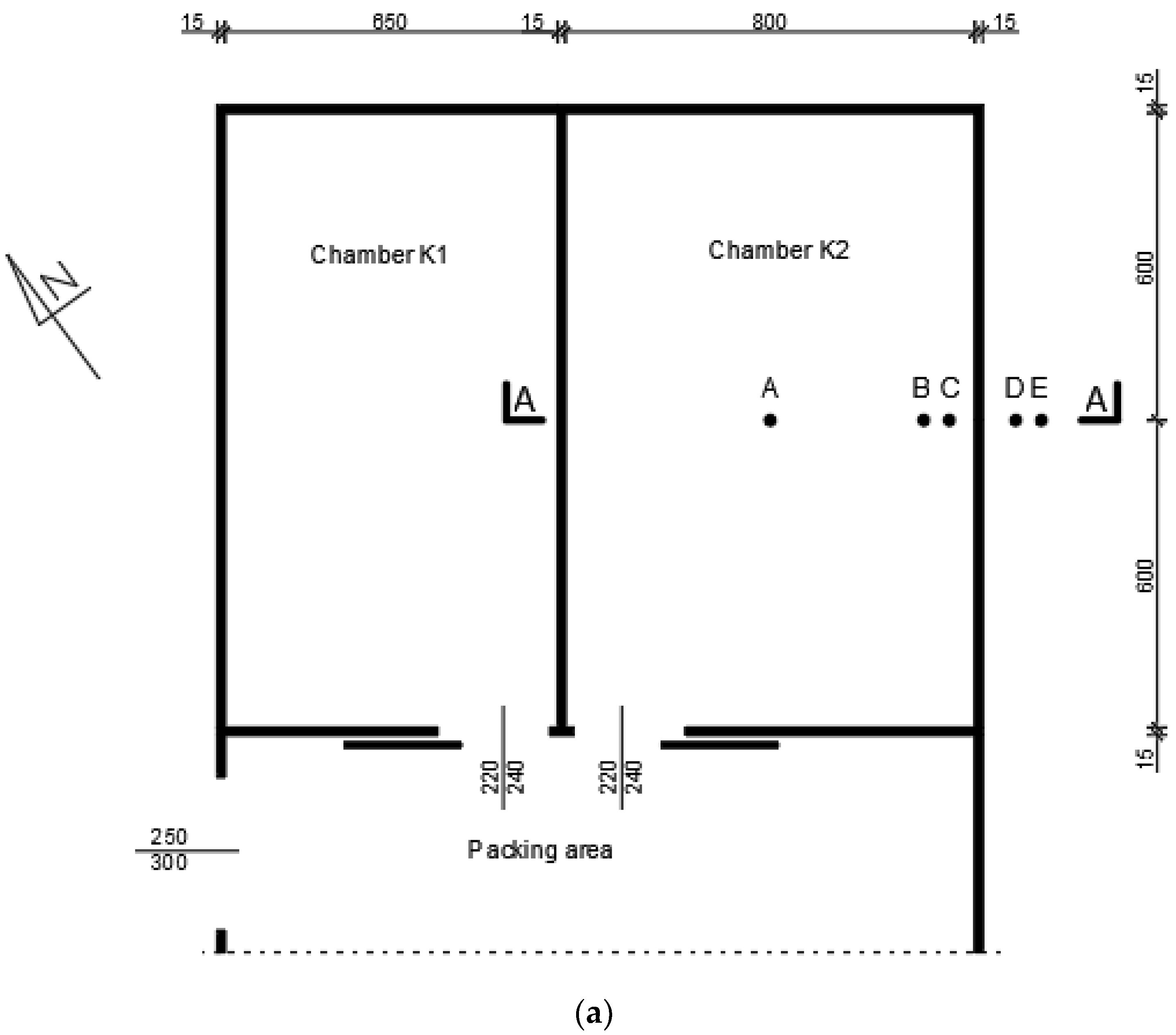
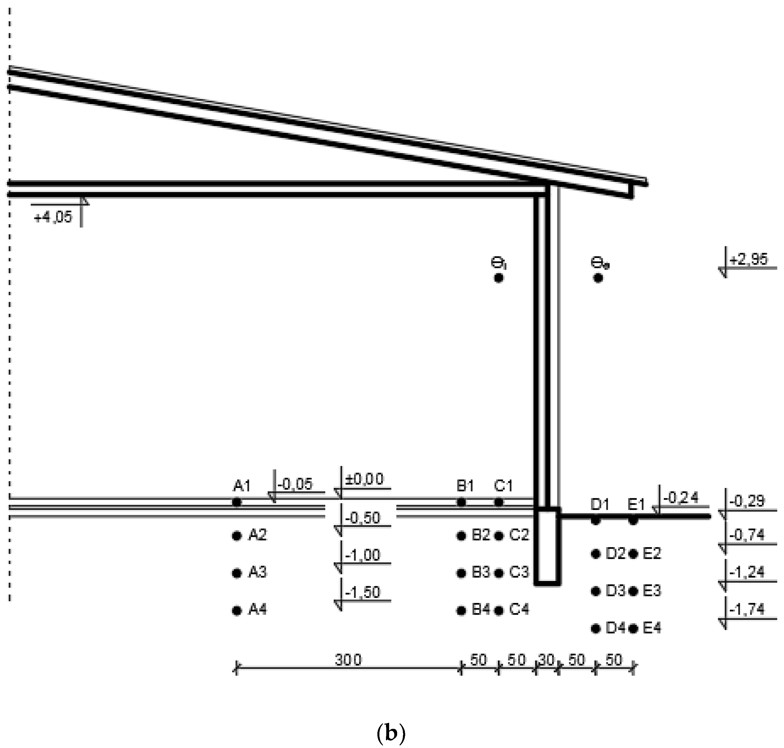
2. Materials and Methods

The experimental studies were conducted in a vegetable cold store in southern Poland. The building has two cold chambers totalling 170 m² (chamber K1—78 m², chamber K2—96 m²) and a 58 m² sorting and packing area. The walls are made of steel H-sections, with sandwich panels between them. The insulating core in the panels is 15 cm XPS. The roof is also steel structure and sandwich panels as in case of the walls. The floor on the ground was made in traditional technology (10 cm cement screed, 4 cm XPS for thermal insulation). The dimensions of cold chambers were adapted to pallet boxes in which carrots (Daucus carota) were stored. During the cooling cycle (from 15 October to 30 June), the indoor air temperature in the chambers was kept at 0.0–4.0 °C, in accordance with recommendations for the stored crops. The cooling system was based on a 20 kW refrigerating unit. An organoleptic soil examination showed that the cold store surrounding includes a 40-cm thick humus (fertile soil) layer, with silty clay below it down to the depth of 2.0 m below ground level. The examination was made using a 2.50 m long geotechnical auger.

The scope of experimental studies included continuous measurements of indoor air temperature, outdoor air temperature, floor temperature, ground temperature under the floor down to the depth of 1.50 m below the floor level, ground temperature in the cold store surrounding down to the depth of 1.50 m below ground level. Twenty-two PT100 sensors with 0.1 °C measurement accuracy were used. These parameters were measured for the chamber K2. The preliminary tests by the authors who analyzed the temperature and humidity conditions in both chambers did not show any statistically significant differences, so it was decided to continue with more accurate studies for the larger chamber (K2). The measurements were automatically recorded at 60-minintervals on a computer hard drive connected to the measuring instruments. The location of measurement points and the cold store layout are presented in Figure 1. The results of experimental studies allowed determining the thermal conditions inside the examined chamber and in the ground below it. The unit heat losses to the ground through the floor were estimated based on the relationship (1), where: Θ_i—indoor air temperature, (°C), Θ_g—ground temperature interpolated linearly between points (A1–C1), (°C), λ_s—thermal conductivity coefficient of soil, the used value was 1.9 W/mK, (EN ISO 6946), R_si—heat penetration resistance, the used value was 0.14 m²K/W. The calculations were made based on the floor temperature measured 0.05 m below its surface and the actual curve of indoor air temperature over time was accounted for. Then, the unit values (W/m²) were added and presented in kWh.

$$q=\frac{{\mathsf{\Theta }}_i-{\mathsf{\Theta }}_g}{\left(\frac{0.05}{{\lambda }_s}\right)+R_{si}} \left[\mathrm{W}·{\mathrm{m}}^{-2}\right]$$

(1)

The next step involved the validation of the calculation model based on the elementary balances numerical method. The complex area of the cold store and the ground was divided into cuboidal balance-differential elements (Figure 2), using the model discretization. For each element, it is possible to calculate the increase of its internal energy, which depends on the temperature change (2), where: ∆Q—internal energy increase of the element, (J), C—total heat capacity of the element, (J·K⁻¹), ∆θ—element temperature rise, (K).

$$\Delta Q=C·\Delta \theta \left[\mathrm{J}\right]$$

(2)

The heat flux flowing through the analyzed area is calculated in non-stationary terms, assuming the time step Δτ (3), where: i—elements number, Φ_ixiyiz,… —heat flux (heat flows) flowing between element i_x i_y i_z and adjacent elements (W).

$$\begin{array}{c}\Delta Q=\mathsf{\Delta }\tau ·({\Phi }_{i_x{i}_y{i}_z,i_{x+1}{i}_y{i}_z}+{\Phi }_{i_x{i}_y{i}_z,i_{x-1}{i}_y{i}_z}+{\Phi }_{i_x{i}_y{i}_z,i_x{i}_y{i}_{z+1}}+{\Phi }_{i_x{i}_y{i}_z,i_x{i}_y{i}_{z-1}}\\ +{\Phi }_{i_x{i}_y{i}_z,i_x{i}_{y+1}{i}_z}+{\Phi }_{i_x{i}_y{i}_z,i_x{i}_{y-1}{i}_z})\end{array}$$

(3)

The computational analysis also takes into account the heat flux density, which is calculated on the basis of Fourier’s law (4), where: $\overrightarrow{\dot{q}}$—heat flux density, (W·m⁻²), λ—the thermal conductivity of the component material, (W·m⁻¹·K⁻¹), $\nabla$—Hamilton’s vector operator, $\nabla \overrightarrow{\theta }$—temperature gradient, (K·m⁻¹).

$$\overrightarrow{\dot{q}}=-\lambda \nabla \overrightarrow{\theta } \left[\mathrm{W}·{\mathrm{m}}^{-2}\right].$$

(4)

In the case of stationary heat flow through the balance-differential element, heat balance ΔQ = 0. For non-stationary flow, the temperature increase with the heat increase phenomenon should be taken into account. The formula for the heat balance can therefore be written as (5), where: ΣΦ—sum of heat flows between individual elements, (J), ${\mathsf{\theta }}^{\mathrm{k}+1}$ —temperature in the time step k + 1, (K), ${\mathsf{\theta }}^{\mathrm{k}}$—temperature in the time step k, (K), Δτ—time step, [s].

$$\Delta Q=\mathsf{\Delta }\tau {\displaystyle \sum }\Phi =C({\mathsf{\theta }}^{\mathrm{k}+1}-{\mathsf{\theta }}^{\mathrm{k}})\left[\mathrm{J}\right]$$

(5)

The next step of activities based on the balance-difference method is to write down the system of balance-difference equations. At this stage, the occurrence of a start condition that describes the temperature distribution in the previous time step should also be taken into account. In addition, the system of balance and difference equations should take into account: the current values of air temperature inside and outside the analyzed object, the temperature of the soil medium, as well as adiabatic planes. The above-mentioned parameters are called boundary conditions. As a result of the discretization of the area in the method of elementary balances, a discrete geometric model with a division grid is obtained. For each of these elements, the energy balance equation can be written using explicit difference quotient, implicit differential quotient and Crank–Nicolson differential quotient. Energy and temperature balance calculations were made for each such element, using a 60-min time step. The calculation model validation was made based on the temperature measured inside and outside the cold store. In relation to the ground, the temperature was the third-type boundary condition. The initial temperature used was the average annual temperature for Krakow which is 8.8 °C. The calculations were made using the WUFIplus^®ver. 3.2.0 software (Fraunhofer Institut fur Bauphysik, Holzkirchen Branch, Germany).The validation results were subjected to a statistical correlation analysis, after checking the distribution normality with the Kolmogorov–Smirnov test, and then using the Spearman’s Rank Test. After the completion of the validation and validation calculations, the variant analysis was started.

The numerical analysis was performed for 13 variants with different technological break duration (in 7-day increments): variant 1—no break (all-year-round cooling), variant 2—7 days, variant 3—14 days, variant 4—21 days, variant 5—28 days, variant 6—35 days, variant 7—42 days, variant 8—49 days, variant 9—56 days, variant 10—63 days, variant 11—70 days, variant 12—77 days, variant 13—84 daysand variant 14—91 days. The physical parameters of construction materials and the ground used in the calculation model are presented in

Table 1. Physical parameters of construction materials and the ground used in calculations.

Specification		Unit	Value
clay	bulk density	kg·m−3	1600
	heat capacity	J·kg−1·K−1	1000
	thermal conductivity	W·m−1·K−1	1.80
fertile soil	bulk density	kg·m−3	1800
	heat capacity	J·kg−1·K−1	1260
	thermal conductivity	W·m−1·K−1	0.90
styrofoam	bulk density	kg·m−3	20
	heat capacity	J·kg−1·K−1	1500
	thermal conductivity	W·m−1·K−1	0.04
concrete	bulk density	kg·m−3	2300
	heat capacity	J·kg−1·K−1	1000
	thermal conductivity	W·m−1·K−1	2.30
sand/gravel	bulk density	kg·m−3	1800
	heat capacity	J·kg−1·K−1	840
	thermal conductivity	W·m−1·K−1	0.90
steel	bulk density	kg·m−3	7900
	heat capacity	J·kg−1·K−1	460
	thermal conductivity	W·m−1·K−1	17.00

Source: PN-EN ISO 6946:2008—Building components and building elements—Thermal resistance and heat transfer coefficient—Calculation method.

.

In addition, in all variants the assumed minimum indoor air temperature was Θ_i,min = 0 °C, maximum indoor air temperature Θ_i,max = 4 °C, minimum indoor air relative humidity Rh_i,min = 80%,and maximum indoor air relative humidity Rh_i,max = 99%. Assumed was also natural air change 0.3 h⁻¹ and infiltration 0.2 h⁻¹. The climatic data for a typical meteorological year for Krakow (TRY) available in WUFIplus^® were used in the calculation variant analysis. Based on the results obtained by Czapp and Charun [26] and by Jedynak [27], the following breathing heat values for the stored carrots were used: for 0 °C—18.9 W/t, for 4 °C—30.5 W/t. The intermediate values were linearly interpolated.

The obtained model validation results were analyzed for mean arithmetic difference in comparison to the measured data. The mean error was determined based on the Formula (2), where: Δθ—mean error, θp—measured temperature, θo—calculated temperature, N—number of measurements.

$$\Delta \theta = \frac{{\displaystyle \sum }\left|{\theta }_p-{\theta }_o\right|}{N}$$

(6)

Precise curves for indoor air temperature, floor temperature and ground temperature were obtained for each variant. The detailed analysis was performed of the cold store energy demand and of the heat exchange with the ground, with particular emphasis on the initial period of the cooling cycle and the whole yearly operation.

3. Results

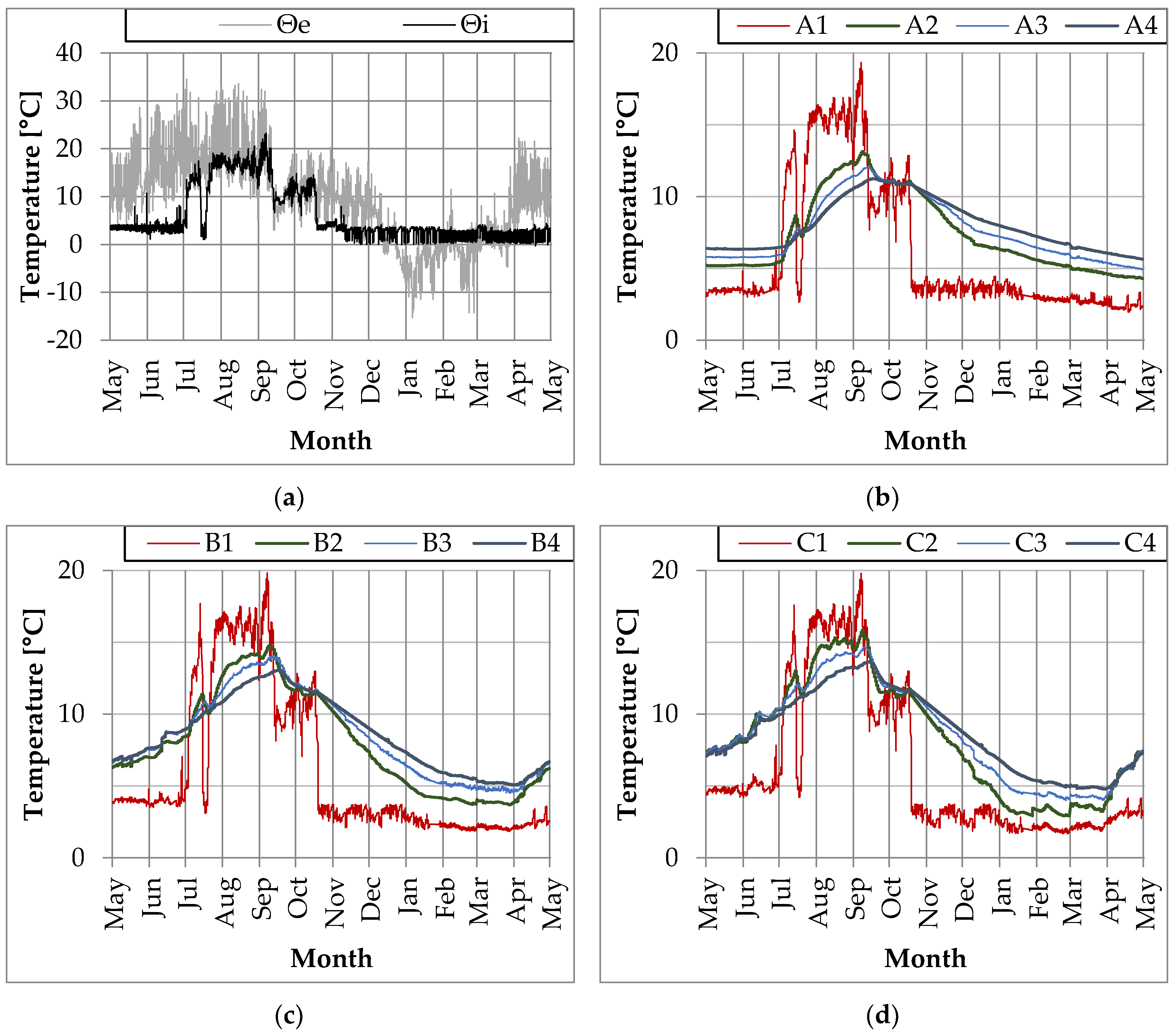
3.1. Experimental Studies

The average outdoor air temperature during the experimental studies conducted from 1 May 2017 to 30 April 2018 was 9.4 °C. The lowest temperature recorded in winter was −15.3 °C. The temperature inside the cold store was kept at 0.4–5.6 °C. During the technological break from the beginning of July to the end of September, the indoor microclimate followed the outdoor microclimate changes. No vegetables were stored in the chamber during that period and the refrigerating units were off, causing the air temperature in the chamber to increase to 15.3 °C in August. The maximum outdoor air temperature in that period was 22.3 °C. In the winter, the average temperature inside the cold store was from 1.0 °C to 1.6 °C, but in the remaining months it was near 4.0 °C (Figure 3a). The floor temperature analysis in point A1 showed that on the last day of the cooling cycle it was 4.2 °C. On the first day of the next cooling cycle, the floor temperature was 11.6 °C and gradually decreased. It was determined that the period necessary to lower the floor temperature to the value from the end of the cooling cycle in the analyzed variant is 18 days (Figure 3b–d). The annual ground temperature amplitude in point E1 was 29.4 °C, but at the depth of 1.5 m in the same measuring line (E4) it was 9.2 °C, which is very close the average annual outdoor air temperature(9.4 °C). The calculation results showed the highest ground temperature in point E1, which was 18.8 °C and was reached in June. The lowest ground temperature (−10.6 °C) was recorded in January in the same measurement point (Figure 3e,f).

The analysis of heat exchange between the indoor and outdoor air and the ground air showed that the greatest heat gains of 27.5 kWh occurred in December. Due to technological break in summer, the heat flow to the ground in July was intensive, reaching the maximum of 37.2 kWh (Figure 4). In total, the ground delivered 1807.9 kWh of energy to the cold store, and the heat losses from the cold store to the ground were 1289.5 kWh in the whole period of study, mainly during the technological break.

The beginning of technological break also marks the beginning of the heating process of the floor and the ground below it. In a cooling facility, this is undesirable because the accumulated energy surplus in the ground directly affects the increased cooling energy demand on the first days of the next cycle. After the cooling cycle ended, the floor in point A1 reached the temperature close to the indoor air temperature after 8 days and 14 h (Figure 5a). The temperature equalization in points B1 and C1 with the indoor air temperature was much quicker. Twenty-two hours had passed since the refrigeration unit was stopped until the temperature in these points reached the comparable value (Figure 5b). Such large differences in the heating time allows a clear separation of the wall zone (up to 1.0 m from the outside wall) and the central zone. The wall zone is very susceptible to the outdoor weather, also to the action of the ground surrounding the cold store building. The results from measurement points located at other depths were also analyzed. The presence of wall zone was equally noticeable there.

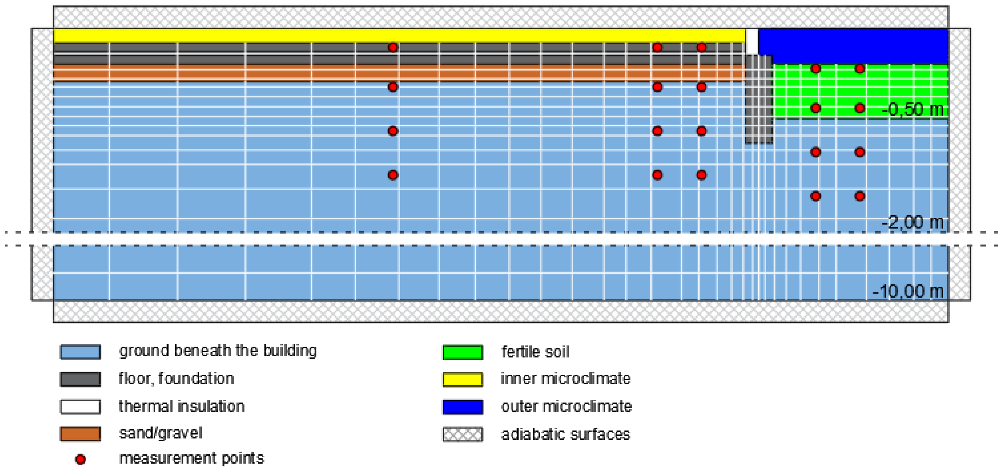
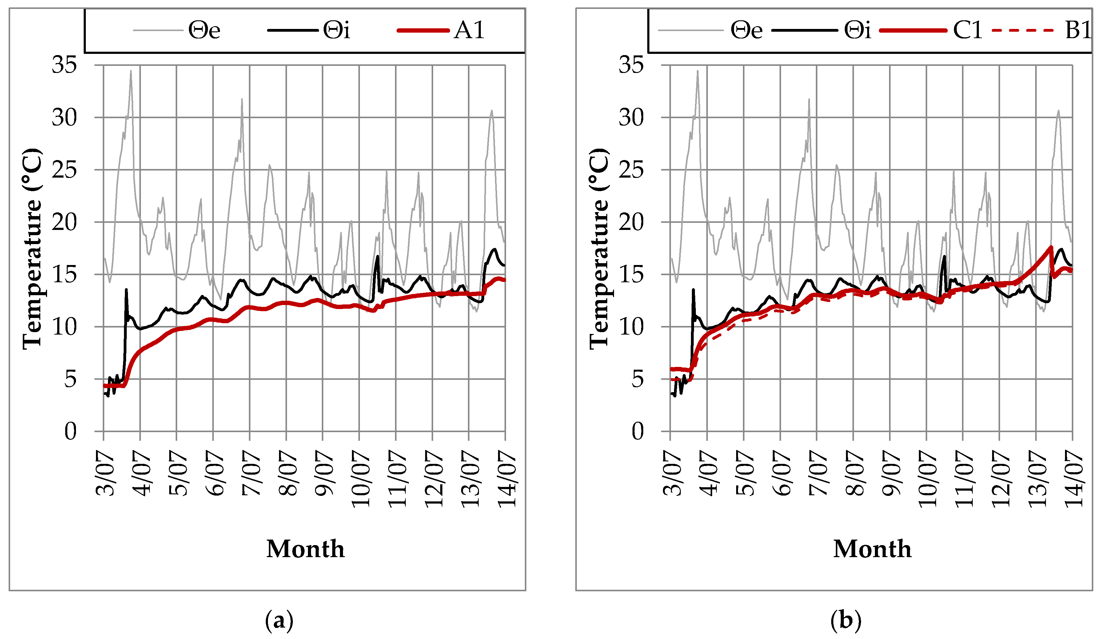
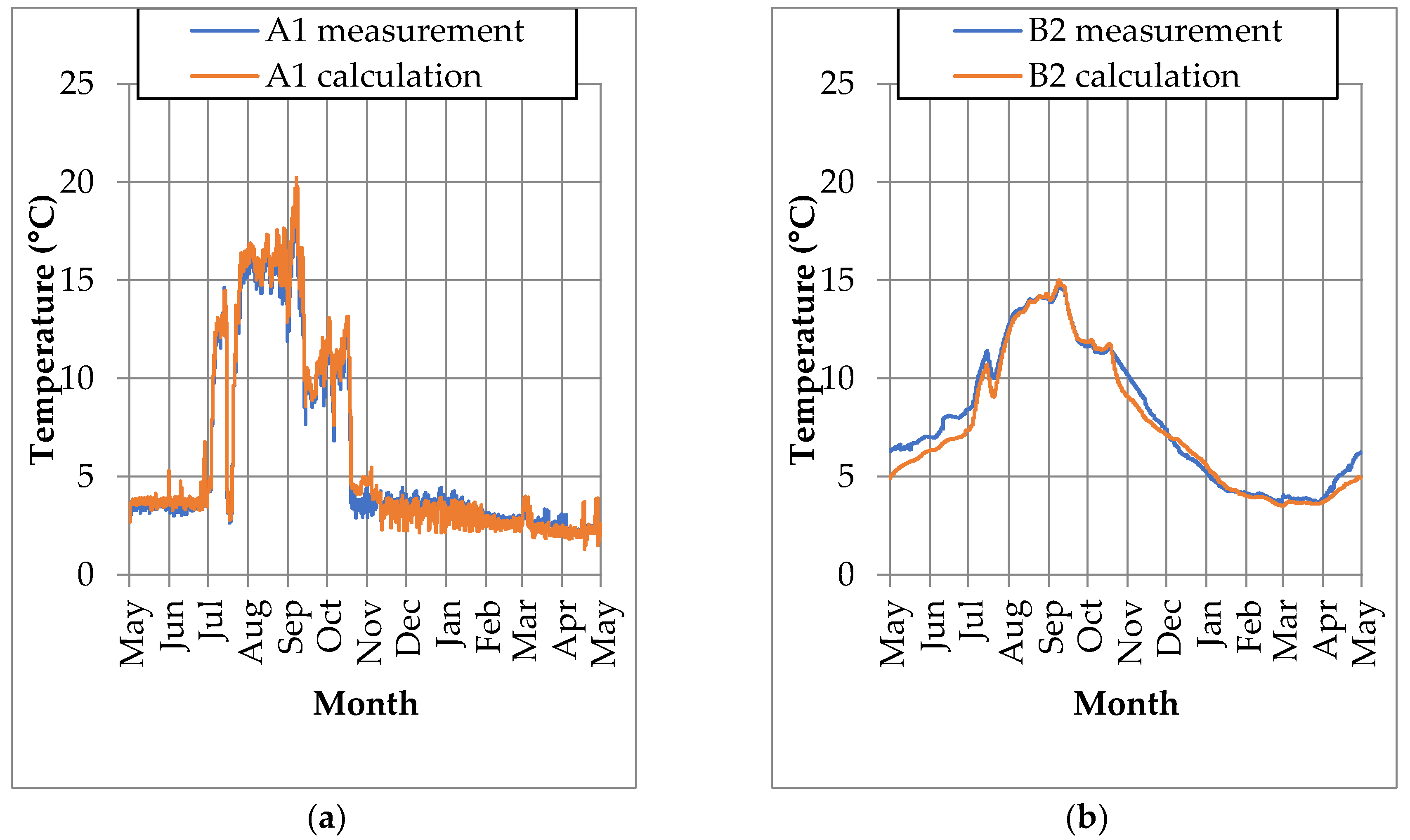
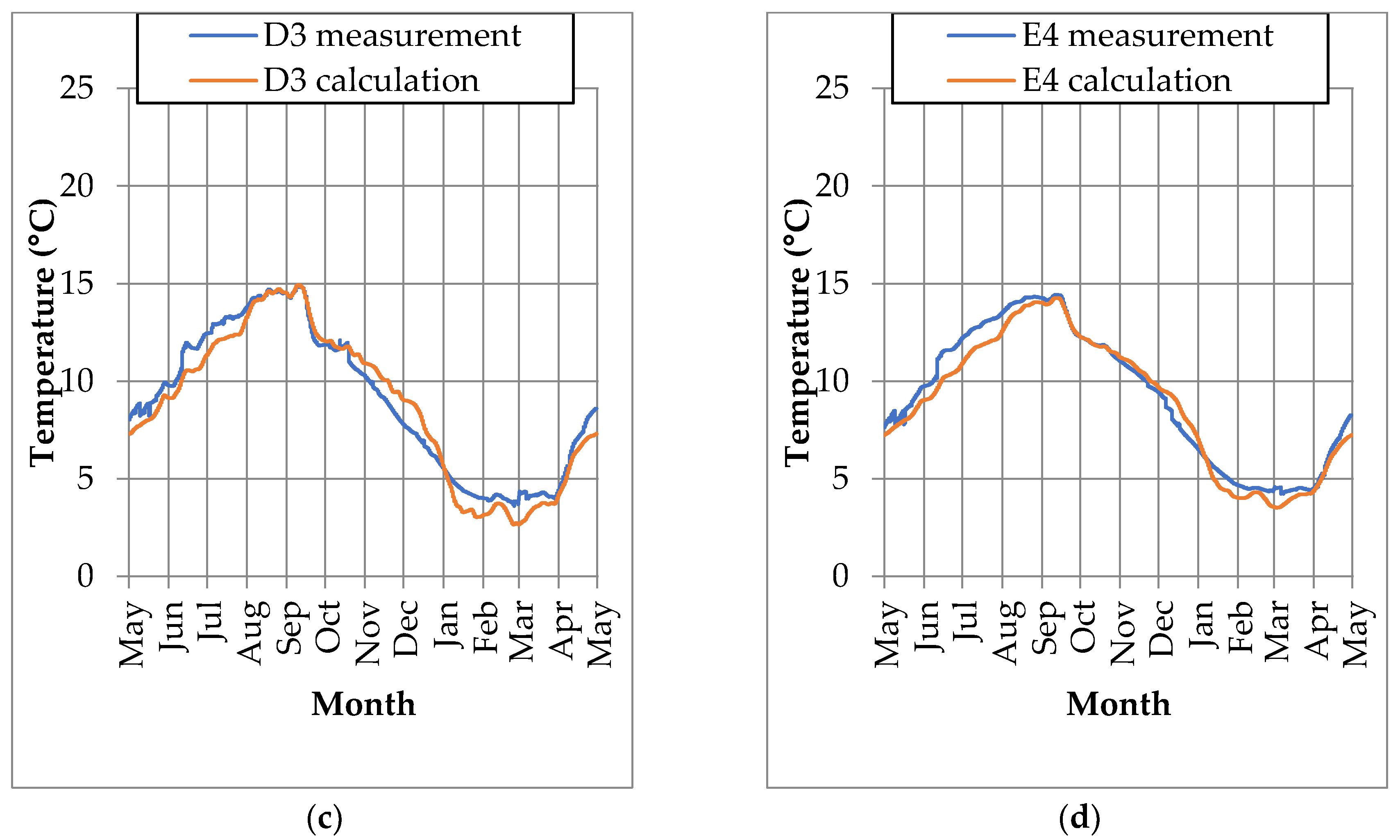
3.2. Calculation Model Validation

The calculations for the analyzed variants were performed using the cold store geometrical model built in the WUFI^®plus, which corresponded to actual dimensions. The first step included the calculation model validation (Figure 6).

Correlation analysis was performed for results obtained from all measurement points based on the Spearman’s Rank Test (the data distribution was not normal). The data distribution normality was tested previously using the Shapiro–Wilk Test. The highest correlation coefficient (0.95–0.99) was determined for measurement points E2, E3, E4, D2, D3, D4, C2, C3, C4, B2, B3, B4and A2, A3 and A4. Consequently, the conformity of calculation and measurement data at the depth of 0.50 m, 1.00 m and 1.50 m can be considered full. In case of points E1 and D1, located 0.05 m below the ground level, and A1, B1 and C1 located under the floor, the correlation coefficient was 0.85–0.88, so the conformity of measurement and calculation data should be considered very high. It should be emphasized that in winter the actual soil temperature at the depth of 0.10 m differed from the calculated values by 11.2 °C in line E and 11.0 °C in line D. The reason was the impossibility of accounting for the snow cover. The differences occurred only for a short time however, and were not significant in relation to the entire period of study. The statistical significance of differences was tested using the Kruskal–Wallis test (p < 0.05). The mean error for all measurement points was in the 1.0–3.0 °C range. The lowest error values in the 1.0–1.8 °C were obtained for the lines located inside the cold store(A, B and C), and the highest in the 1.4–3.0 °C for the outside lines (E and D). The greatest mean error was found in point E1 (3.0 °C).

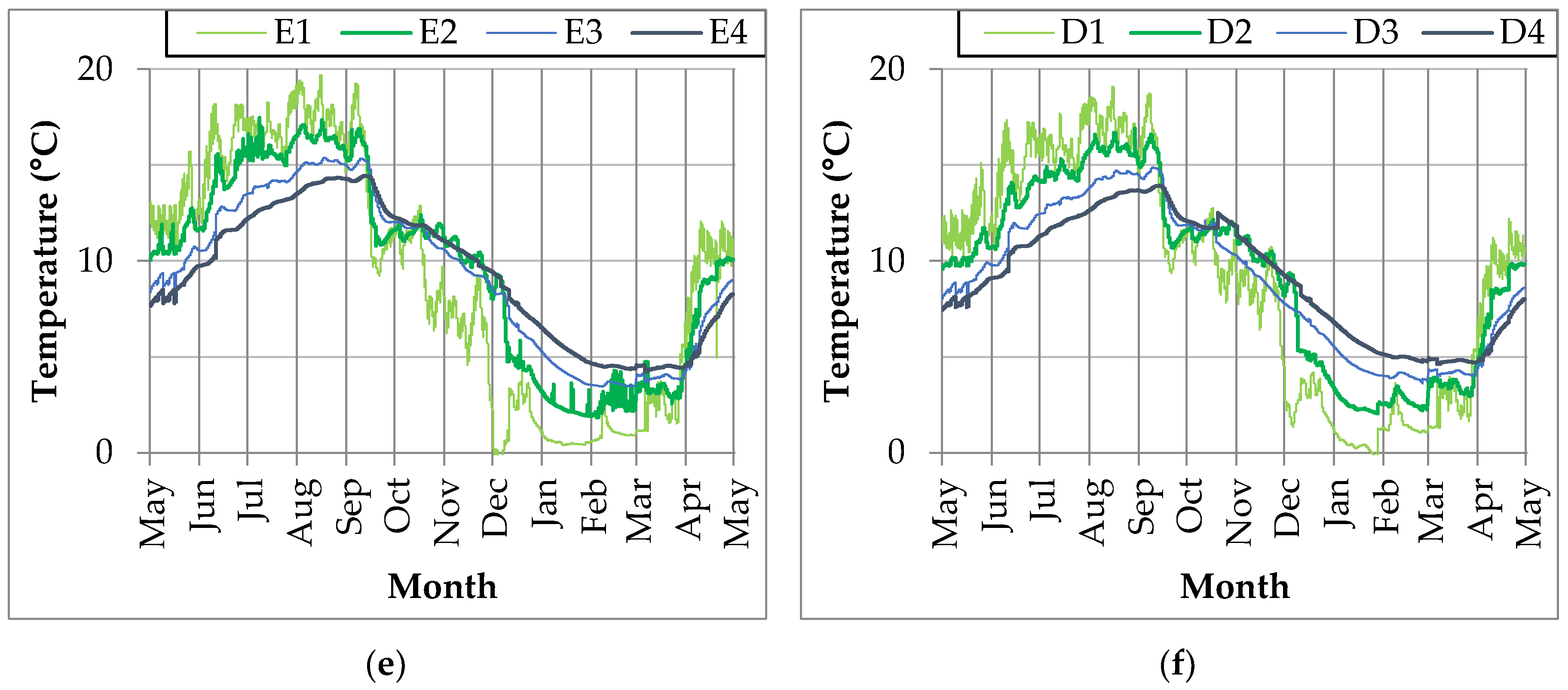
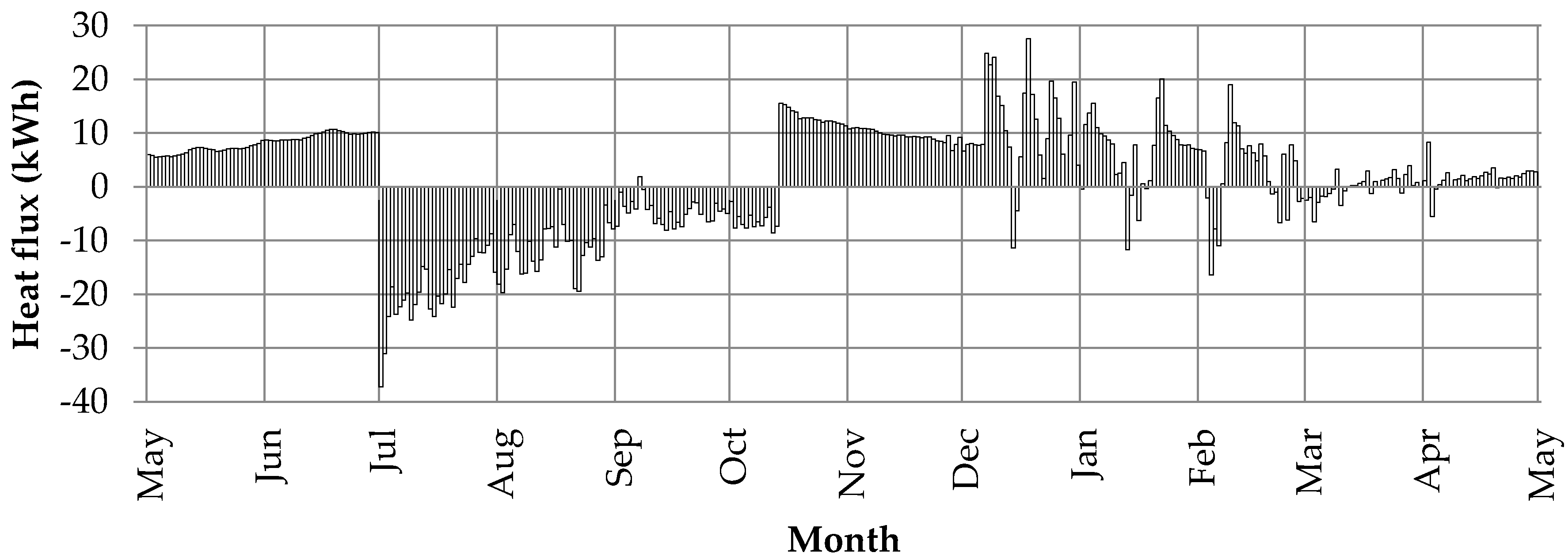
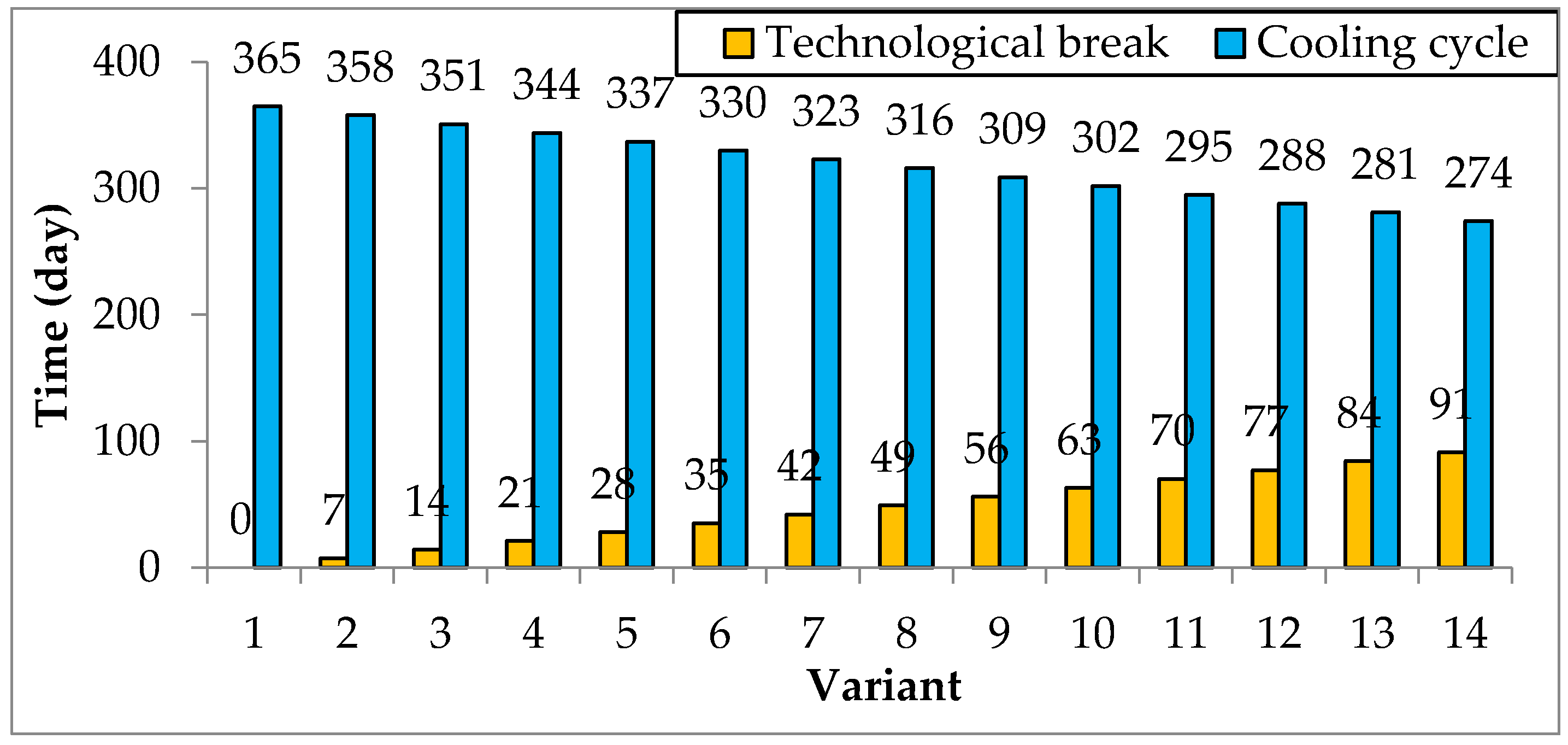
3.3. Calculation Variant Analysis

The calculation analysis was performed on 14 variants differing in terms of the technological break duration (Figure 7). Due to a large amount of data, the variant analysis results are given as average values and for the whole year, for better illustration of global differences between individual variants.

In all variants the action of low temperature inside the cold store was clearly noticeable down to the depth of 0.50 m relative to the floor level. The impact of indoor microclimate on the thermal conditions of the ground under the floor gradually disappeared at lower levels (1.0 m and 1.5 m). The annual floor temperature amplitude (variant 1) in point A1 was 3.9 °C (Figure 8a). In case of 91-day technological break (variant 14) the temperatures of the floor and the ground under it were in a much wider range. The annual temperature amplitude in point A1 was 13.9 °C, in point A2—8.3 °C, A3—7.2 °C and A4—6.3 °C (Figure 8b). The technological break duration therefore has a significant impact on the thermal conditions of the floor and ground under it.

The simulation results have showed that the technological break duration has a significant impact on the cold store energy demand and the heat exchange with the ground, but also on the cooling time of the ground under the floor. Absence of technological break (variant 1) results in a decrease of energy gains from the ground by 20% relative to a three-month technological break (variant 14). The impact of technological break duration was clearly seen in terms of energy losses from the cold store to the ground (Figure 9). In case of a 91-day technological break (variant 14), the energy losses to the ground were 1289.5 kWh/a, while in case of absence of technological break (variant 1) this value was ninefold lower (147.5 kWh/a). On the cooling cycle end (30 June—variant 14), the ground temperature in point A2 was 5.2 °C. During 91 days of technological break, the floor and the ground under it was gradually heated. The free flow of outdoor air into the cold store was assumed in order to reflect the actual conditions. The assumed end of technological break was 30 September. On this day, the soil temperature in point A2 was 11.0 °C. After the start of the cooling cycle, an intensive flow of the heat to the ground took place and the time necessary to cool down the ground in point A2 to the same temperature as on 30 June was 143 days. For comparison, in case of a seven-day technological break (1–7 July), the time necessary to cool down the ground to the temperature as before the technological break was 1 day and 14 h (variant 2). An interesting relationship was obtained for a 70-day technological break (variant 11). In this case, the time necessary to cool down the ground was 141 days and was similar to results in variants 12–14. The reason is mainly the impact of the outdoor microclimate on the microclimate inside the cold store. In variant 11, the technological break ends in early September. In this time of the year, the outdoor air temperature falls, so even without the cooling system operation, the ground under the floor and the ground surrounding the building cools down spontaneously.

The analysis of indoor air temperature simulation results showed that a six-week technological break (variant 6) allows maintaining the average indoor air temperature at the 3.95 °C level (

Table 2. Average temperature [°C] of indoor air, floor and the ground for 14 calculation variants.

Variant	Θi	C1	C2	C3	C4	B1	B2	B3	B4	A1	A2	A3	A4
1	3.29	3.41	5.82	6.06	6.26	3.40	5.69	5.94	6.13	3.39	5.36	5.60	5.79
2	3.46	3.58	5.90	6.15	6.34	3.57	5.77	6.02	6.22	3.55	5.46	5.69	5.89
3	3.52	3.75	5.98	6.23	6.43	3.74	5.85	6.11	6.31	3.72	5.56	5.78	5.99
4	3.38	3.91	6.06	6.32	6.52	3.91	5.94	6.19	6.40	3.88	5.65	5.88	6.08
5	3.80	4.08	6.14	6.40	6.61	4.08	6.02	6.28	6.49	4.05	5.75	5.97	6.18
6	3.95	4.25	6.22	6.49	6.70	4.25	6.10	6.37	6.58	4.21	5.85	6.06	6.28
7	4.11	4.42	6.30	6.57	6.78	4.42	6.19	6.45	6.67	4.38	5.94	6.16	6.38
8	4.27	4.59	6.38	6.66	6.87	4.59	6.27	6.54	6.76	4.54	6.04	6.25	6.47
9	4.42	4.75	6.46	6.74	6.96	4.76	6.35	6.62	6.85	4.70	6.14	6.34	6.57
10	4.72	4.92	6.54	6.83	7.05	4.93	6.44	6.71	6.94	4.87	6.23	6.44	6.67
11	4.95	5.09	6.62	6.91	7.14	5.10	6.52	6.80	7.03	5.03	6.33	6.53	6.76
12	5.11	5.26	6.69	7.00	7.22	5.27	6.60	6.88	7.11	5.20	6.43	6.62	6.86
13	5.35	5.42	6.77	7.08	7.31	5.44	6.69	6.97	7.20	5.36	6.52	6.72	6.96
14	5.59	5.70	6.92	7.18	7.41	5.68	6.82	7.09	7.33	5.65	6.63	6.89	7.14

).

The extension of technological break (variants 7–14) contributes to the average annual indoor air temperature exceeding 4.0 °C, which significantly increases the cooling energy demand, particularly on the first days of the cooling cycle. The analysis of the floor temperature results (points A1–C1) showed that the technological break longer than four weeks causes the average floor temperature to exceed 4.0 °C. Therefore, the optimum solution is technological break lasting 7–35 days (variants 2–5). At a shorter technological break, the facility can be used for storing young vegetables in the summer period.

4. Discussion

Agricultural buildings used periodically allow numerous technological and operational modifications. They can contribute to rational management of energy necessary to maintain a given building type [28,29]. Current state of knowledge shows that the share of the ground in the total energy balance of residential and industrial buildings is about 5–10% [17]. As a result of continuous development of digital technologies, numerical methods are increasingly used for modelling and forecasting of physical phenomena [30,31,32]. However, computer simulations have some limitations and do not account for all factors which in reality can affect the studied parameters [23]. Validation of calculation models requires the results of field measurements encompassing the period of at least one year. Without such results, the simulation results could be burdened with a large error, particularly in case of untypical buildings as agricultural ones, and the obtained data should be considered estimates. There are studies that indicate the need for verification of the impact of the cold store thermal insulation in different floor location variants on the intensity of heat exchange with the ground and the share of the soil in the total building energy balance [30,33,34]. There has been no scientific paper to date which discusses the impact of the technological break in the cooling cycle on the heat exchange with the ground and the building energy management. This paper should be considered a case study and a foundation for further, more elaborated analyses. The studies in this regard on agricultural buildings are difficult because there are no relevant standards which could regulate some issues as it is the case in residential and industrial buildings. The agricultural buildings have different indoor condition, particularly air temperature and relative humidity. Depending on the building structure, area of its envelopes and most importantly its intended use, the percent share of envelopes in contact with the ground can significantly affect the energy gains and losses and the building energy management. In the future, the authors plan to use the model for further energy analyses related to the influence of other factors, such as. the type of stored products and their distribution on the shaping of selected parameters of the microclimate of the cold store. For this it is planned to use the CFD model.

5. Conclusions

The paper includes a multivariant analysis of the duration of technological break between the cooling cycles in a vegetable cold store located in southern Poland on the heat exchange with the ground. Due to absence of available standards which would allow a precise determination of the heat flux through the ground in such facilities, a numerical elementary balances method was used. The advantage of this approach was obtaining results for 14 variants in non stationary conditions, taking into account actual climatic conditions. The results of experimental studies showed that the conditions inside the cold store were stable and appropriate for stored crops. The technological break took place from the beginning of July to the end of September and the microclimate inside the cold store was shaped passively depending on the changes of the outdoor microclimate. The results of field measurements of the indoor and outdoor air temperatures and the ground temperature were used to validate the calculation model in the WUFI^®plus software, and then to verify the conformity of the calculated results with the real results. After numerous validation calculations, a satisfactory level of conformity of calculated and measured results was obtained. The validated model was used in a simulation of the indoor microclimate, ground temperature and the heat exchange with the ground for all 14 variants. The calculations were made in a non stationary approach. The calculation model validation was performed based on the results of field studies of the indoor and outdoor air temperature and the ground temperature in five measurement lines at the depth of 0.05, 0.50, 1.00 and 1.50 m. The obtained validation results showed a very high correlation between the measured and calculated data and absence of significant differences (p < 0.05). The annual floor temperature amplitude for variant 1 (cooling all year long) in point A1 was 3.9 °C. In case of three-month technological break (variant 14) the temperatures of the floor and the ground under it were in a much wider range. The annual temperature amplitude in point A1 was 13.9 °C, in point A2—8.3 °C, A3—7.2 °C and A4—6.3 °C. The technological break duration has therefore a significant impact on the thermal conditions of the floor and ground under it. The analysis of simulation results showed also that absence of technological break (variant1) results in a decrease of energy gains from the ground by 20% relative to a three-month technological break. The analysis of the floor temperature calculations (points A1–C1) showed that the technological break longer than four weeks causes the average floor temperature to exceed 4.0 °C. Therefore, the optimum solution is technological break lasting 7–35 days. At a shorter technological break, the facility can be used for storing young vegetables in the summer period.

References

1. Zhang, Z.; Sun, D. Effect of cooling methods on the cooling efficiencies and qualities of cooked broccoli and carrot slices. J. Food Eng. 2006, 77, 320–326. [Google Scholar] [CrossRef]
2. Sun, D.-W.; Wang, L. Experimental investigation of performance of vacuum cooling for commercial large cooked meat joints. J. Food Eng. 2004, 61, 527–532. [Google Scholar] [CrossRef]
3. Phillips, K.M.; Council-Troche, M.C.A.; McGinty, R.C.; Rasor, A.S.; Tarrago-Trani, M.T. Stability of vitamin C in fruit and vegetable homogenates stored at different temperatures. J. Food Compos. Anal. 2016, 45, 147–162. [Google Scholar] [CrossRef]
4. Mazzeo, T.; Paciulli, M.; Chiavaro, E.; Visconti, A.; Pellegrini, N. Impact of the industrial freezing process on selected vegetables—Part II. Colour and bioactive compounds. Food Res. Int. 2015, 75, 89–97. [Google Scholar] [CrossRef]
5. Wu, Z.S.; Zhang, M.; Wang, S. Effects of high pressure argon treatments on the quality of fresh-cut apples at cold storage. Food Control 2012, 23, 120–127. [Google Scholar] [CrossRef]
6. Ambaw, A.; Delele, M.A.; Defraeye, T.; Ho, Q.T.; Opara, L.U.; Nicolai, B.M.; Verboven, P. The use of CFD to characterize and design post-harvest storage facilities: Past, present and future. Comput. Electron. Agric. 2013, 93, 184–194. [Google Scholar] [CrossRef] [Green Version]
7. East, A.R.; Smale, N.J.; Trujillo, F.J. Potential for energy cost savings by utilizing alternative temperature control strategies for controlled atmosphere stored apples. Int. J. Refrig. 2013, 36, 1109–1117. [Google Scholar] [CrossRef]
8. Liu, Y.; Langer, V.; Hogh-Jensen, H.; Egelyng, H. Life Cycle Assessment of fossil energy use and greenhouse gas emissions inChinese pear production. J. Clean. Prod. 2010, 18, 1423–1430. [Google Scholar] [CrossRef]
9. Allais, I.; Alvarez, G. Analysis of heat transfer Turing mist Schilling of a packed Bed of spheres simulating foodstuffs. J. Food Eng. 2001, 49, 37–47. [Google Scholar] [CrossRef]
10. Alvares, G.; Flick, D. Modelling turbulent flow and heat transfer using macroporous medium approach used to predict cooling kinetics of stacks of food products. J. Food Eng. 2007, 80, 391–401. [Google Scholar] [CrossRef]
11. Verboven PHoang, M.I.; Baelmans, M.; Nicolai, B.M. Airflow through beds of apples and chicory roots. Biosyst. Eng. 2004, 88, 17–125. [Google Scholar] [CrossRef]
12. Baerdemaeker, D.J.; Delele, M.A.; Verboven, P.; Bart, M. Multiscale modeling of postharvest storage of fruit and vegetables in a plant factory context. IFAC Proc. Vol. 2011, 44, 616–620. [Google Scholar] [CrossRef] [Green Version]
13. Delele, M.A.; Verboven, P.; Ho, Q.T.; Nicolai, B.M. Advances in mathematical modeling of postharvest refrigeration processes. Stewart Postharvest Rev. 2010, 2, 1–8. [Google Scholar]
14. Nawalany, G.; Sokołowski, P. Analysis of hygrothermal conditions of external partitions in an underground fruit store. J. Ecol. Eng. 2016, 17, 75–82. [Google Scholar] [CrossRef]
15. Nawalany, G.; Sokołowski, P.; Herbut, P.; Angrecka, S. Development of selected parameters of microclimate in a stand alone cellar plunged into soil. J. Ecol. Eng. 2017, 18, 156–161. [Google Scholar] [CrossRef]
16. Radoń, J.; Bieda, W.; Lendelova, J.; Pogran, S. Computational model of heat exchange between dairy cow and bedding. Comput. Electron. Agric. 2014, 107, 29–37. [Google Scholar]
17. Nawalany, G.; Bieda, W.; Radoń, J.; Herbut, P. Experimental study on development of thermal conditions in ground beneath a greenhouses. Energy Energy 2014, 69, 103–111. [Google Scholar] [CrossRef]
18. Nawalany, G.; Radoń, J.; Bieda, W.; Sokołowski, P. Influence of selected factors on heat exchange with the ground in a greenhouse. Trans. ASABE 2017, 60, 479–487. [Google Scholar]
19. Martin, S.; Canas, I. A comparison between underground wine Cellary and aboveground storage for the aging of Spanish wines. Trans. ASABE 2006, 49, 1471–1478. [Google Scholar] [CrossRef]
20. Erol, S.; Francois, B. Multilayer analitical model for vertical ground heat exchanger with groundwater flow. Geothermics 2018, 71, 294–305. [Google Scholar] [CrossRef]
21. Zhao, B. Study on heat transfer of ground heat exchanger based on wedgelet finite element method. Int. Commun. Heat Mass Transf. 2016, 74, 63–68. [Google Scholar] [CrossRef]
22. Kupiec, K.; Larwa, B.; Gwadera, M. Heat transfer in horizontal ground heat exchangers. Appl. Therm. Eng. 2015, 75, 270–276. [Google Scholar] [CrossRef]
23. Akkurt, G.G.; Aste, N.; Borderon, J.; Buda, A.; Calzolari, M.; Chung, D.; Costanzo, V.; Del Pero, C.; Evola, G.; Huerto-Cardenas, H.E.; et al. Dynamic thermal and hygrometric simulation of historical buildings: Critical factors and possible solutions. Renew. Sustain. Energy Rev. 2020, 118, 109509. [Google Scholar] [CrossRef]
24. Dahlem, K.-H. Ein neues Berechnungsverfahren für den Wärmeverlusterdreichberührter Bauteilezum Grundwasser. Teil 1; Gesundheits Ingenieur, Haustechnik-Bauphysik-Umwelttechnik: Munchen, Germany, 2001; Volume 4, pp. 173–178. [Google Scholar]
25. Dahlem, K.-H. Ein neues Berechnungsverfahren für den Wärmeverlusterdreichberührter Bauteilezum Grundwasser. Teil 2; Gesundheits Ingenieur, Haustechnik-Bauphysik-Umwelttechnik: Munchen, Germany, 2001; Volume 5, pp. 234–238. [Google Scholar]
26. Czapp, M.; Charun, H. Principles of Developing a Heat Balance of Cooling Rooms; University Publishing House of Koszalin University of Technology: Koszalin, Poland, 1995; pp. 343–349. [Google Scholar]
27. Jedynak, T. Mechanizacja Prac w Magazynach Owoców i Warzyw; CRS: Warsaw, Poland, 1970. [Google Scholar]
28. Rossi, P.; Gastaldo, A.; Riva, G.; De Carolis, C. Progetto Re Sole; Centro Ricerche Produzioni Animali (CRPA): Reggio Emilia, Italy, 2013. [Google Scholar]
29. Nawalany, G.; Sokołowski, P. Improved Energy Management in an IntermittentlyHeated Building Using a Large Broiler House inCentral Europe as an Example. Energies 2020, 13, 1371. [Google Scholar] [CrossRef] [Green Version]
30. Bambara, J.; Athienitis, A.K. Energy and Economic Analysis for greenhouse Ground Insulation Design. Energies 2018, 11, 3218. [Google Scholar] [CrossRef] [Green Version]
31. Dong, C. Heat Loss via Concrete Slab Floors in Australian Houses. Procedia Eng. 2017, 205, 108–115. [Google Scholar]
32. Nawalany, G.; Sokołowski, P.; Michalik, M. Experimental Study of Thermal and Humidity Conditions in a Historic Wooden Building in Southern Poland. Buildings 2020, 10, 118. [Google Scholar] [CrossRef]
33. Hyung-Kweon, K.; Geum-Choon, K.; Jong-Pil, M.; Tae-Seok, L.; Sung-Sik, O. Estimation of Thermal Performance and Heat Loss in Plastic Greenhouses with and without Thermal Curtains. Energies 2018, 11, 578. [Google Scholar] [CrossRef] [Green Version]
34. Jakubowski, T.; Krolczyk Jolanta, B. Method for the reduction of natural losses of potato tubers during their long-therm storage. Sustainbility 2020, 12, 1048. [Google Scholar] [CrossRef] [Green Version]
Figure 1. Location of measurement points in the cold store: (a) plan, (b) section I–I: A, B, C, D, E—measuring lines, A1–A4, B1–B4, C1–C4, D1–D4, E1–E4—soil temperature measurement points, Θi, Θe—air temperature measurement points.
Energies 13 04970 g001aEnergies 13 04970 g001b
Figure 2. Section of the modelled facility with the division network and layout of soil temperature calculation points (model from WUFIplus® software).
Energies 13 04970 g002
Figure 3. Temperature curves for indoor Θi and outdoor Θe air(a) and for floor and the ground in measurement points A1–A4 (b); B1–B4 (c); C1–C4 (d); E1–E4 (e); D1–D4 (f).
Energies 13 04970 g003aEnergies 13 04970 g003b
Figure 4. Heat exchange between the cold store and the ground.
Energies 13 04970 g004
Figure 5. Temperature curves for the indoor and outdoor air and floor in points A1 (a) and B1 and C1 (b) in the initial period of technological break.
Energies 13 04970 g005
Figure 6. Calculated and actual floor and ground temperatures in the cold store and its surrounding (a) measurement point A1; (b) measurement pointB2; (c) measurement pointD3; (d) measurement pointE4.
Energies 13 04970 g006aEnergies 13 04970 g006b
Figure 7. Duration of cooling cycle and technological break in individual variants.
Energies 13 04970 g007
Figure 8. Maximum, minimum and annual average temperature in point A1: (a) variant 1; (b) variant 14.
Energies 13 04970 g008
Figure 9. Energy gains and losses through the ground for 14 calculation variants.
Energies 13 04970 g009