Uncertainty Analysis of Greenhouse Gas (GHG) Emissions Simulated by the Parametric Monte Carlo Simulation and Nonparametric Bootstrap Method

Abstract

Uncertainty of greenhouse gas (GHG) emissions was analyzed using the parametric Monte Carlo simulation (MCS) method and the non-parametric bootstrap method. There was a certain number of observations required of a dataset before GHG emissions reached an asymptotic value. Treating a coefficient (i.e., GHG emission factor) as a random variable did not alter the mean; however, it yielded higher uncertainty of GHG emissions compared to the case when treating a coefficient constant. The non-parametric bootstrap method reduces the variance of GHG. A mathematical model for estimating GHG emissions should treat the GHG emission factor as a random variable. When the estimated probability density function (PDF) of the original dataset is incorrect, the nonparametric bootstrap method, not the parametric MCS method, should be the method of choice for the uncertainty analysis of GHG emissions.

1. Introduction

In accordance with the Paris Accord, many countries around the world set up voluntary goals for mitigating greenhouse gas (GHG) emissions and implement various action plans, including related research to achieve the goals. Many industrial sectors set up the goals and action plans to comply with the Paris Accord. They include, among others, goals related to energy, industrial processes and product use, agriculture, forest and other land use, and waste. The energy sector, including the transportation sector, formulated three different policy scenarios for the carbon emission goal in 2050 and computed GHG emissions for each scenario [1]. Vázquez-Rowe et al. [2] estimated GHG emissions of cement production in three relevant national cement plants to identify the main GHG mitigation strategies throughout the whole supply chain in industrial processes and the product use sector. Baek et al. [3] developed a GHG emission quantification procedure for dairy cow systems based on a life cycle assessment (LCA) approach incorporating the Intergovernmental Panel on Climate Change (IPCC)’s GHG emission computation equations in the agriculture sector. The waste sector computed GHG emissions from the composting and solid waste treatment processes and suggested recommendations for improving the current waste management policy [4].

The above literature [1,2,3,4] adopted the same methodological approach for estimating GHG emissions in each sector [5,6]. This approach involves integrating information on the level of human activity (i.e., activity data) with the quantified emission coefficients per unit activity (i.e., emission factor) [7]. Therefore, a model used extensively for the computation of GHG emissions from different sources in a given sector is a linear model, where the activity data are multiplied by the emission factor.

Recently, uncertainty analysis of a mathematical model such as the greenhouse gas (GHG) emission estimation model is receiving increasing attention. GHG has an environmental impact that is categorized as global warming impact, one of the many life cycle impact categories in life cycle assessment (LCA). When estimating GHG emissions, it is always necessary to evaluate and quantify the uncertainties of estimates. Uncertainty analyses help analysts identify how accurate the estimations are and the likely range in which the true value of the emissions fall [8].

Uncertainty refers to the difference between the true value and the measured value. All input random variables to the mathematical model have uncertainty, be it systematic or random [9,10]. Uncertainty of the input random variables often refers to error. As such, this paper defines the uncertainty of the model output as an uncertainty and the uncertainty of the input random variables as an error.

A model is a mathematical description of the real-world phenomenon. A model can have any number of parameters, and they are interrelated through various mathematical operations. Parameters (e.g., activities, processes, and emission factors) refer to any input random variables comprising a mathematical model. Error in the parameter originates from the lack of knowledge about the true value of the parameter [11]. These errors can vary widely from a few percent to orders of magnitude [12]. Errors associated with the parameters are bound to increase due to the compounding effect of the errors in the parameters. The compounding effect is often termed error propagation [8,13,14].

The variance of the mathematical model output is a measure of uncertainty of the model output. Statistics such as the confidence interval (CI) and relative uncertainty (U) are used widely for assessing the uncertainty [10]. The relative uncertainty is defined as a ratio between the half-width of the CI to the sample mean of the model output [10]. McMurray et al. [8] recommended that analysts apply the CI method for calculating uncertainty, considering that other methods such as the coefficient of variation (CV) underestimated uncertainty.

Uncertainty analysis methods often used for the mathematical model output are the error propagation, the Monte Carlo simulation (MCS) method and the bootstrap method. However, the error propagation method is intended for computing the variance of the model output, not for the CI. Many prior studies used the error propagation method for computing the uncertainty not based on the CI [9,10,14].

The MCS is run using algorithms that generate stochastic (i.e., random) values based on the probability distribution function (PDF) of the original dataset [8]. The normal distribution of the original dataset is often assumed [8]. However, non-normal assumptions such as log-normal assumptions were also made frequently [9,12,15].

Two widely used uncertainty analysis methods, the parametric MCS method and the non-parametric bootstrap method, were chosen to assess the uncertainty of GHG emissions. The parametric MCS method requires estimation of the probability distribution of the original dataset of a parameter, while the nonparametric bootstrap method does not. Lee et al. [16] showed that the nonparametric bootstrap method gives smaller relative uncertainty over the parametric MCS method. However, this study did not estimate the probability distribution of the parameter data but assumed normal and lognormal distributions. In addition, they relied on commercial software for performing the MCS.

The error propagation equation ignoring the covariance among the parameters in a model was recommended for use to calculate the uncertainties of GHG emissions from individual input uncertainty estimates [17]. However, the covariance among the parameters can be significant in most cases and cannot be ignored. Besides, there is a matrix operation that allows calculation of the variance–covariance matrix of the input parameter data [13,16]. A newer version of the IPCC guidelines [10] recommends MCS as the more detailed uncertainty analysis method.

Estimation of the probability distribution is faced with difficulties because of the limited number of observations of the original dataset. Inaccurate PDF will lead to inaccurate MCS output such that accurate estimation of PDF is a prerequisite for proper use of the parametric MCS method.

There are several studies on the uncertainty analysis of GHG emissions based on the MCS method with an assumed probability distribution. Hong et al. [18] stated that the statistical features of the total carbon emissions can be determined through its probability distribution when performing MCS. They assumed the beta distribution of the observed data in the construction industry. Others rely on expert judgment for choosing probability distribution [3,9].

However, it is rare to find studies that estimate probability distribution explicitly for MCS. Lee, et al. [16,19] used the Anderson–Darling (AD) test to estimate the probability distribution of the input variable. The p-value and AD statistics were used to test the null hypothesis for the assumed probability distributions. McMurray et al. [8] described a step-by-step approach for estimating PDF for GHG emissions using the goodness-to-fit test of the parameter data. Thus, there is a need to assess the effect of estimating probability distribution on the uncertainty of the model output.

The emission factor is often expressed as a single point estimate, not an interval estimate. However, the value of the emission factor can vary. Thus, there is a need to assess the effect of the varying emission factor (i.e., treating it as a random variable) on the uncertainty of the model output.

As the number of observations (n) of an original dataset increases, its variance decreases. When increasing n of the dataset, there would be a certain n where the variance of the model output, and subsequently the value of U, no longer decreases with the increase in n. Thus, there is a need to assess the effect of n of the original dataset on the value of U and mean of the model output.

Therefore, the objective of this study was to assess: (i) the effect of the number of observations of an original dataset; (ii) the effect of treating the emission factor as random variable; (iii) the effect of a probability distribution; and, (iv) the effect of different uncertainty analysis methods—all on the uncertainty of the model output or GHG emissions.

2. Materials and Methods

2.1. Mathematical Model

GHG emissions are estimated by multiplying the input variables by their corresponding GHG emission factors. Input variables are the input and output of materials and energies from a product system such as resources consumed and emissions discharged as well as activities such as transportation. Of these, those related to GHG emissions are chosen together with their corresponding GHG emission factor for use in Equation (1).

A mathematical model in Equation (1) for computing GHG emissions from a system is a linear combination of the input variables.

$$\mathrm{Z}=\mathrm{AX}$$

(1)

where $\mathrm{Z}$ = the model output (e.g., GHG emission), $\mathrm{A}$ = the coefficient vector, and $\mathrm{X}$ = the input variable matrix.

The model output has uncertainty originating from the errors of the input variables. The errors of the input variables to the mathematical model propagate such that the uncertainty of the model output increases [14,20]. The variance of Z measures the uncertainty of Z. Since Z is a linear combination of A and X, Equation (2) computes the variance of Z [21]. Most of the time, the input variables are not independent such that variance computation should include the covariance of X. Equation (2) is also known as the error propagation equation [20,21].

$$\mathrm{var}\left(\mathrm{Z}\right)=\mathrm{var}\left(\mathrm{AX}\right)=\mathrm{Avar}\left(\mathrm{X}\right)A^T$$

(2)

where $\mathrm{var}\left(\mathrm{X}\right)$ = the variance–covariance matrix of $\mathrm{X}$, and $A^T$ = transpose of A.

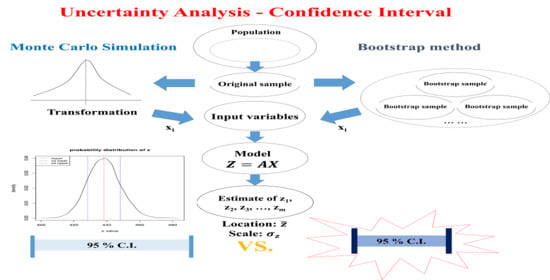
In order to reduce errors of the input variables X in Equation (1), many observations of a dataset should be collected for each input variable. However, this is infeasible and impractical. As such, stochastic modeling is necessary where many observations of the input variables are generated artificially, and these observations are used to compute the value of Z by Equation (1).

Application of the uncertainty analysis method, the MCS method and the bootstrap method to Equation (1) yields many Z values, expressed as z (numerical value of the random variable Z). These z values are used to compute statistics of interest such as the mean, variance, confidence interval, relative uncertainty, bias, and standard error, among others.

2.2. Uncertainty Analysis by the Parametric MCS Method

MCS is a random experimentation based on random sampling from the uniform distribution that generates uniform random variates. These variates are then transformed into the random variates of the cumulative distribution function (CDF) of the original dataset [14]. The random variates generated are used to solve Equation (1).

MCS can be performed in four steps: (i) generate uniform random variates vector, u, from the uniform distribution of (0,1); (ii) the u vector is transformed into the corresponding values of CDF of the original dataset, the x vector, which are random variates of the original dataset distribution; (iii) this process repeats many times (e.g., 10,000 times) and generates many sets of x vectors; (iv) these x vectors are used to solve Equation (1) to obtain z and z vector. Statistics of interest such as the bias, standard error, CI, and U are computed from the z vector.

The use of the MCS method requires estimation of the probability distribution of the original dataset. Fitting distribution consists of choosing a probability distribution model that describes the dataset, finding parameter estimates for that distribution, and the goodness-of-fit test [14,22]. This requires judgment and expertise, and needs an iterative process of distribution choice, parameter estimation, and quality-of-fit assessment [22].

Before choosing a probability model for a given dataset, graphical techniques such as histograms, density estimate, empirical CDF, quantile–quantile (Q–Q) plot, and probability–probability (P–P) plot can be used to suggest the type of probability distribution [16]. Goodness-of-fit tests indicate whether a dataset comes from a specific probability distribution based on the hypothesis test [23].

The fitdistrplus package of R [22,24] was used to choose the probability distribution. The graphical comparison of multiple fitted distributions (cdfcomp) was used by plotting the empirical cumulative distribution and fitted distribution functions (y-axis) against the values of X (x-axis). Other types of plots such as the Q–Q plot (qqcomp) representing the empirical quantiles (y-axis) against the theoretical quantiles (x-axis) were also made, but are not presented here.

Akaike’s information criterion (AIC) and Schwarz Bayesian information criterion (BIC) are widely used indices for the probability distribution selection [25]. Kolmogorov–Smirnov, Cramer-von Mises and Anderson–Darling statistics [26] were also considered to assess the goodness of fit. Gofstat function was used to calculate these statistics [24].

All these statistics were computed, and a probability distribution having the smallest indices and statistic (i.e., distance) was identified. In addition, visual examination of the CDF plots focused not only on both tails of the plot but also on the center of the distribution plot. The probability distribution showing the smallest AIC/BIC criterion and smallest goodness-of-fit statistics (distance) and that which was closest to the empirical CDF was chosen as the probability distribution of the original dataset.

2.3. Unertainty Analysis by the Nonparametric Bootstrap Method

Relatively small samples generally provide very reliable information about the shape of the population. The bootstrap method treats this sample as a population and takes repeated samples with replacements from it; these are bootstrap samples and they give reliable insight into various sample estimates, and reliable confidence intervals can be constructed from these estimates [27]. The bootstrap is a widely applicable and extremely powerful statistical tool that can be used to quantify the uncertainty associated with a given estimator [27,28].

The standard error of an estimator is difficult to estimate in reality. Most of the time, there is no simple formula for the standard error such as the standard error of the sample mean $(\sigma /\sqrt{n}$) [19,29].

The estimated variance of the R-bootstrapped estimates gives standard deviation, and this was used to compute the standard error of the estimator [28]. The diagonal elements of the square root of the variance–covariance matrix are the standard deviation of the bootstrapped datasets [30]. The bias of an estimator is the difference between the mean of the bootstrapped datasets and that of the original dataset [28,31]. With these, the confidence interval of Z is computed [32].

Bootstrapping consists of four steps: (i) collect a sample dataset of size n from the population (original dataset of size n); (ii) draw a bootstrapped sample of size n from the original dataset with a replacement and repeat bootstrap sampling R times; (iii) compute the statistics of interest for each bootstrapped dataset, and there will be a total of R estimates of the estimator; (iv) compute statistics of interest such as the standard error and CI with the R bootstrapped datasets and the original dataset.

In practice, a bootstrap analysis in R can be implemented in three steps [28]: (i) create a function that computes the statistic of interest; (ii) use the boot() function [33] in R to perform bootstrapping by repeatedly sampling from the original dataset with the replacement; and (iii) compute the variance, standard error, bias, CI and U of the model output Z using the bootstrapped datasets and original dataset.

3. Results and Discussion

The feed data for dairy cows were used as the input data to the mathematical model for computing GHG emissions [16]. Six different types of feed to cow and corresponding emission factors were used. These are dry cow feed, lactating cow feed, straw, soybean meal, electricity, and diesel. The corresponding emission factors are 0.38, 0.64, 0.95, 0.71, 0.50, 3.3 kg CO₂-eq/kg (kwh for electricity, liter for diesel), respectively. There are six different batches of the dataset, and all are subsets of the dataset of n = 72 (

Table A1. The feed and utility input variables and their values of dairy cow.

Month	Feed for Dry Cows 1	Feed for Lactating Cows 1	Straw 1	Soybean Meal 1	Electricity 2	Diesel 3
Mon.	X1	X2	X3	X4	X5	X6
1	114	299	54	13	161	5
2	260	411	13	17	113	5
3	278	320	34	18	121	3
4	236	676	23	46	160	22
5	248	741	38	14	225	5
6	183	384	33	16	216	5
7	358	443	35	13	109	6
8	172	786	27	19	125	10
9	83	294	33	14	134	5
10	73	221	18	16	27	4
11	8	241	16	19	35	5
12	57	239	5	4	138	13
13	114	343	26	17	103	4
14	260	365	25	14	109	3
15	278	367	33	19	112	3
16	236	422	31	12	128	5
17	248	380	32	19	120	4
18	183	405	30	20	133	4
19	358	405	29	18	131	5
20	172	389	31	22	119	4
21	83	387	30	15	111	4
22	73	390	29	12	112	5
23	8	418	34	21	126	5
24	57	407	29	23	121	5
25	114	377	24	20	121	3
26	260	348	22	16	99	4
27	278	371	28	21	116	4
28	236	389	29	18	119	5
29	248	383	29	17	118	4
30	183	396	30	19	123	4
31	358	400	34	21	123	4
32	172	403	33	23	126	6
33	83	406	34	28	126	4
34	73	425	34	16	129	4
35	8	415	36	17	133	4
36	57	401	29	14	116	4
37	114	390	26	19	115	4
38	260	358	22	19	106	5
39	278	417	18	23	145	5
40	236	432	33	21	141	5
41	248	455	32	15	144	4
42	183	436	32	18	136	6
43	358	349	26	17	108	4
44	172	401	27	18	122	5
45	83	376	29	18	115	4
46	73	410	29	22	122	5
47	8	361	29	10	112	5
48	57	378	29	24	121	5
49	114	408	31	17	122	5
50	260	355	31	9	112	4
51	278	366	26	15	107	4
52	236	405	34	13	123	5
53	248	340	32	23	109	3
54	183	384	31	18	116	2
55	358	454	34	21	136	3
56	172	406	32	21	119	5
57	83	416	33	15	123	4
58	73	423	29	20	119	4
59	8	380	27	19	118	4
60	57	383	29	17	123	4
61	114	355	30	14	107	4
62	260	351	25	16	109	1
63	278	381	28	22	117	7
64	236	381	31	15	123	6
65	248	444	34	25	138	5
66	183	403	27	19	122	4
67	358	406	33	16	120	3
68	172	454	38	20	142	5
69	83	448	37	26	126	4
70	73	380	23	22	115	3
71	8	386	35	22	114	4
72	57	375	22	14	113	4
EF 1	0.38	0.64	0.95	0.71	0.50	3.3

Notes: ¹ kg CO₂-eq/kg; ² kWh electricity/head-month; ³ kg diesel/head-month.

). Each subset has a differing length of n, where n is 12, 24, 36, 48, 60, and 72.

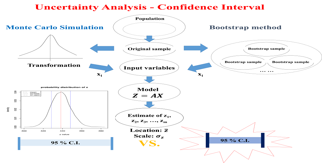
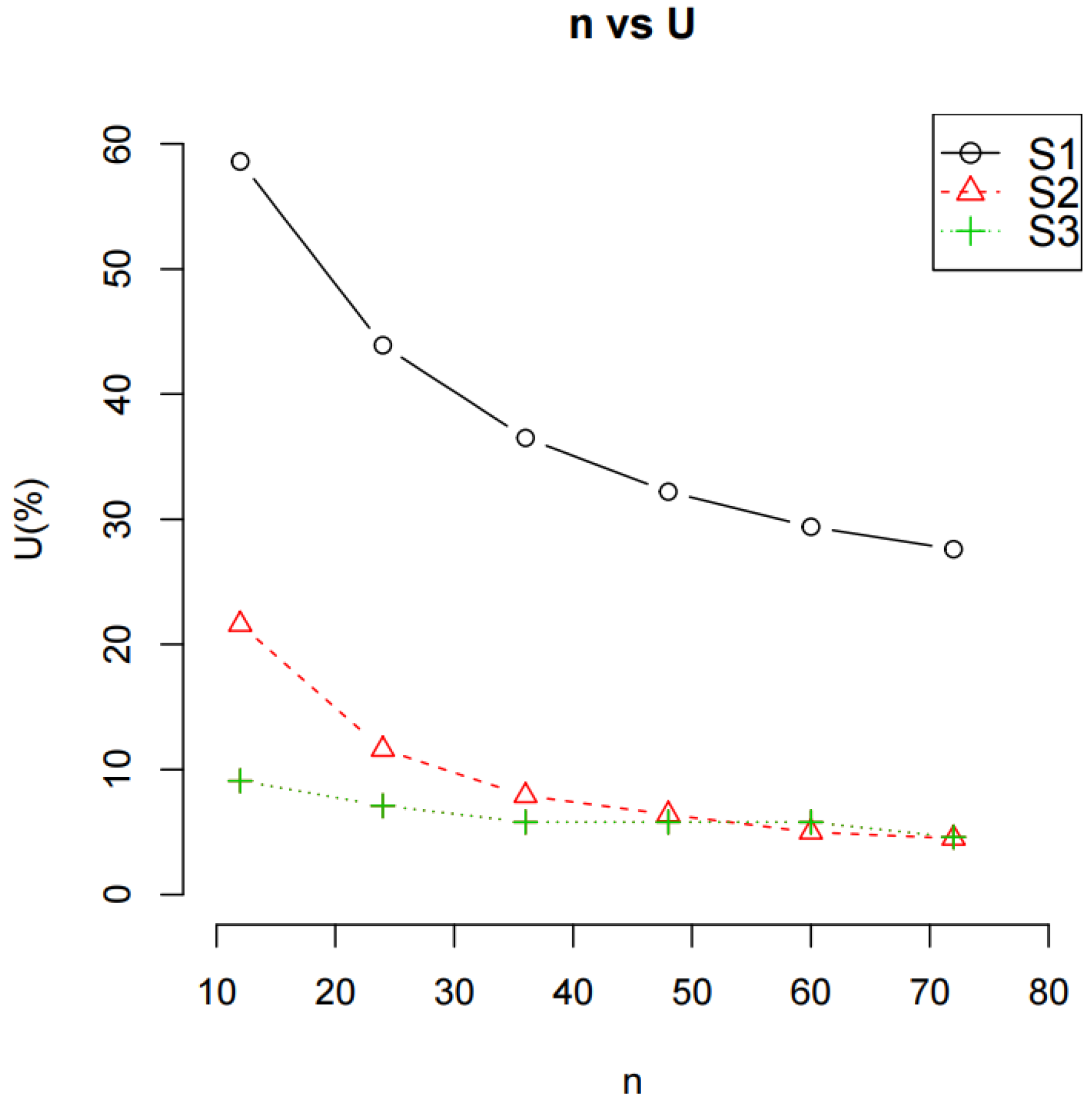
3.1. The Effect of the Size of the Dataset (n) on the Uncertainty of the Model Output

In order to assess the effect of the size of the dataset (n) on the uncertainty of the model output, Z, three different scenarios for computing the mean and variance of Z (S1, S2, and S3) were made. The bootstrap method was used for the assessment. Scenario S1 computes the mean and variance of Z using Equation (1) and the error propagation equation in Equation (2), respectively, and no bootstrapping was used. Here, X is the input variable matrix consisting of six columns of the dataset, each column data with the size of n. Scenario S2 computes the mean and variance of Z by bootstrapping X while keeping A constant. The bootstrapped datasets together with the original dataset were used for the computation of the statistics.

Scenario S3 computes the mean and variance of Z similar to S2. Unlike S2, however, coefficient vector A was treated as a random variable. Since A was constant initially, a linear transformation is needed to generate random variates from A. Uniform distribution of [EF × f_ab, EF × (f_ab + 2 × (1 − f_ab))] was assumed, where EF is an emission factor and “f_ab” is a multiplication factor to generate uniform variates for A. The value of f_ab varies from 0.0 to 1.0. Scenario S3 computes the mean and variance of Z by bootstrapping both X and A.

Table 1. Summary of the three different scenarios.

Scenario	Var(Z) Calculation	Treatment of A Vector
S1	Error propagation method (no bootstrapping)	Keeping A vector constant
S2	Bootstrapping X matrix only	Keeping A vector constant
S3	Bootstrapping both X matrix and A vector	Treating A vector as a random variable

shows the summary of the three different scenarios described above.

Figure 1 and Figure 2 show the effect of the size of a dataset (n) of the three different scenarios on the U and mean of Z (i.e., the mean GHG emission), respectively. As n increases, the U and mean GHG emission decrease in all three scenarios and reach an asymptotic value. The plot of U vs. n in Figure 1 shows that the U decreased rapidly initially and then reached a minimum value. This indicates that the increase in n decreases the variance of Z and remains unchanged beyond a certain number of n (here, n ≥ 48). The plot of the mean GHG emission vs. n in Figure 2 shows the same trend.

Scenario S3 exhibited the lowest U and the mean GHG emission followed by Scenario S2 and then Scenario S1. This was quite obvious for the U, while less obvious for the mean GHG emission. The variance of Z was the smallest in Scenario S3 (bootstrapping both A and X), followed by Scenario S2 (bootstrapping X only), and was the largest in Scenario S1 (no bootstrapping). This indicates that bootstrapping reduces the variance of Z.

In the case of the mean GHG emission, Scenario S1 and S2 exhibited essentially the same trend. However, Scenario S3 reached an asymptotic value when n was 36, while scenarios S1 and S2 reached the same asymptotic value when n was equal to and/or greater than 60. A significant decrease in the mean GHG emission when the number of data is small indicates that the mean GHG emission is not stable. As such, there is a certain number of observations of a dataset required before a stable mean GHG emission can be reached. In this case, the number of observations was 36 for Scenario S3 and 60 for scenarios S1 and S2.

Tong et al. [34] investigated the effect of sample size on the bias of the confidence interval of the original dataset and the bootstrapped dataset. Using the original dataset to construct a confidence interval for quantifying the uncertainty of GHG emissions may lead to a significant bias when the sample size is small. Compared with this, the bootstrapped confidence intervals have smaller interval mean and smaller interval standard deviation for small sample size (n < 30) under non-normal distributions [34]. This suggests that there will be a certain sample size above which the uncertainty of the model output reached a stable value.

3.2. The Effect of Treating the Emission Factor (Coefficient Vector) as a Random Variable on the Uncertainty of the Model Output

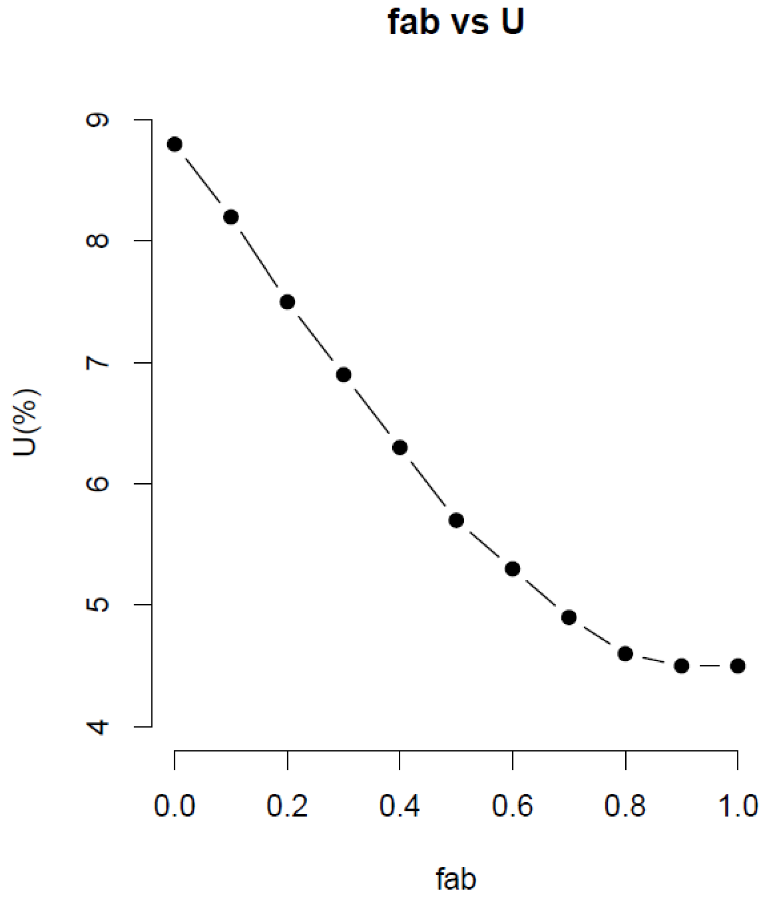
Figure 3 shows the effect of f_ab on the U and mean GHG emission for the bootstrap method. The value of U decreases by approximately 90% when f_ab varies from 0.0 to 1. This indicates that the variability of the coefficient affects the U. When f_ab was 0.0, the U was 8.8%. When f_ab reached 0.9, no further changes occurred to the U. Thus, treating the coefficient as a random variable increases the uncertainty of Z or U. This is because the variance of the dataset increases due to increased variance of the coefficient.

Meanwhile, the mean GHG emission remains flat in all values of fab, i.e., 440.2 kg CO₂-eq/head-year at f_ab of 0.0, and 438.5 kg CO₂-eq/head-year at f_ab of 1.0. This indicates that treating the coefficient in the mathematical model as a random variable does not alter the mean of Z. It affects adversely, however, the uncertainty of Z. The varying coefficient case yielded higher uncertainty of Z over the constant coefficient case.

3.3. The Effect of Probability Destribution on the Uncertainty of the Model

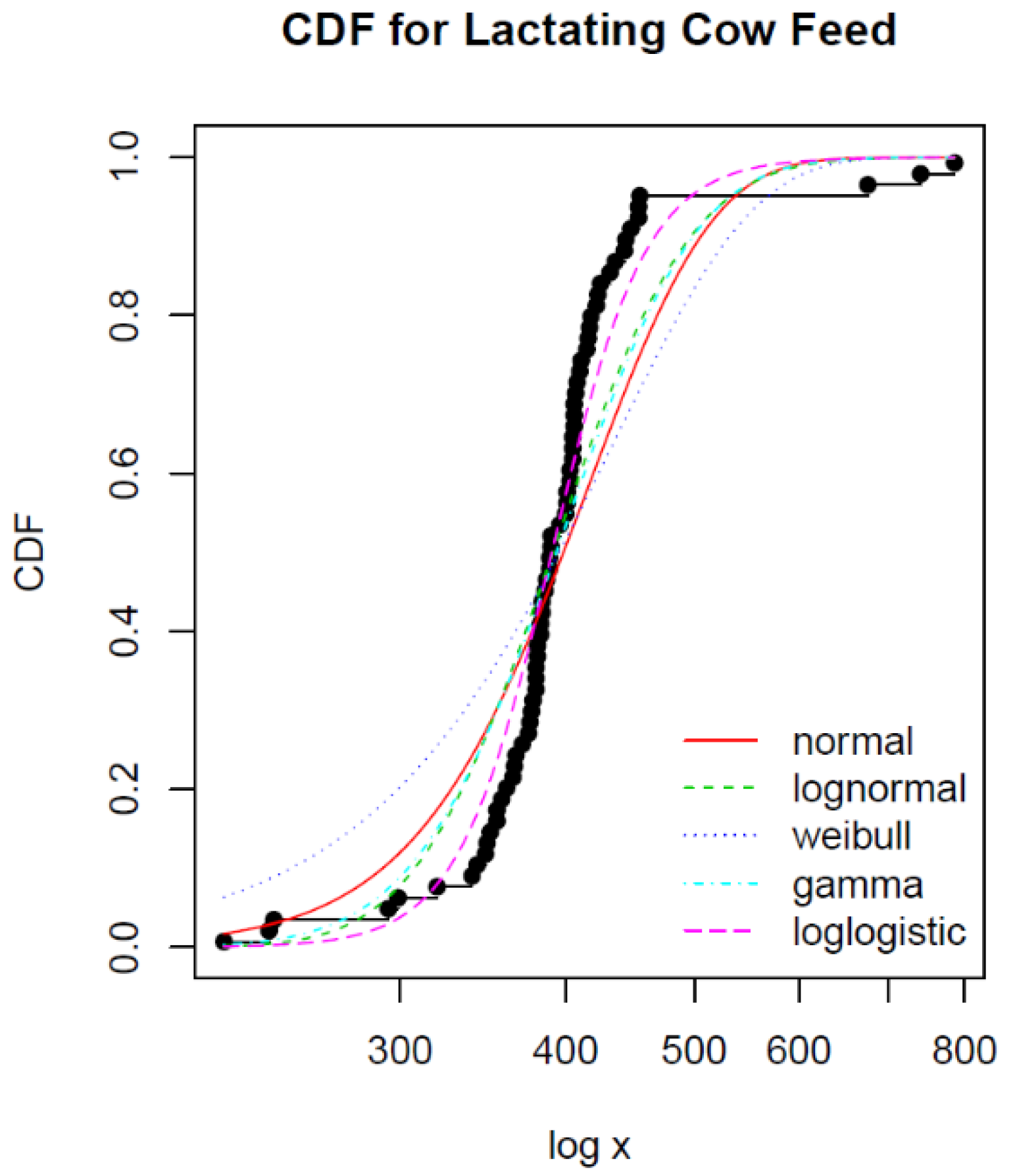
The very first step in performing MCS is the estimation of the probability distribution of the original dataset. Figure 4 shows the empirical and theoretical CDF (y-axis) against the input values of x (x-axis) for the lactating cow feed dataset.

Akaike’s information criterion (AIC) provides a measure of the model fit, with smaller values of AIC indicating a better-fitting model. The same is true for the Bayesian information criterion (BIC).

Table 2. Goodness-of-fit criterion for the lactating cow feed data case.

Goodness-of-Fit Criterion	Probability Distribution
	normal	lognormal	Weibull	gamma	loglogistic
AIC	845.9	826.5	864.9	830.9	803.5
BIC	850.5	831.1	869.5	835.4	808.1

shows that loglogistic distribution fits best for the lactating cow feed dataset, judging from the smallest AIC and BIC values among the five distributions tested.

From the five different distributions shown in Figure 4, loglogistic distribution also exhibits close proximity to the empirical CDF in all ranges of the input values of X (x-axis). This is in agreement with the AIC and BIC values in Table 2. Thus, loglogistic distribution was chosen for the distribution of the lactating cow feed dataset. This process heavily depends on the goodness-of-fit criterion as well as the CDF plots. Inevitably, this process involves judgment call and thus implies difficulties associated with the estimation of the probability distribution of the dataset.

Table 3. Chosen distribution of the data with relevant statistics.

Column (Data) Name	Distribution	Mean	Sd 1	Shape	Scale
Dry cow feed	Weibull			1.57	189.82
Lactating cow feed	loglogistic			12.28	390.54
Straw	normal	29.36	6.36
Soy bean meal	loglogistic			6.97	17.81
Electricity	loglogistic			10.92	120.97
Diesel	loglogistic			6.20	4.36

¹ Standard deviation.

shows the chosen distribution of the original dataset for the six columns of the dataset. It lists statistics of each distribution.

3.4. Comparison of the Confidence Interval Computation Method

The confidence interval is the base for assessing the uncertainty of Z. The U is based on the CI width. Three different CI computation methods including the percentile method, normal method, and basic method were tested to examine any difference among them. The bootstrap method was used for the test.

Table 4. Comparison of the confidence interval computation methods.

Statistic	Percentile	Normal	Basic
95% CI	(418.13–458.57)	(418.55–458.00)	(416.88–457.32)
CI width	40.44	39.45	40.44
U (%)	4.64	4.51	4.64

shows that the three CI computation methods produce essentially the same results.

Orloff and Bloom [35] emphasized that the percentile method is preferred to the other methods. This is because the $\overline{X}-\mathsf{\mu }$ distribution is approximated by the $\overline{X^{*}}-\overline{X}$ distribution, where $\mathsf{\mu }$, $\overline{X}$ and $\overline{X^{*}}$ are the true mean, mean of the original dataset, and mean of the bootstrapped data, respectively. Tong et al. [34] compared different methods for computing the confidence interval; they were the normal method, percentile method, bias-corrected percentile method, and bias-corrected accelerated percentile (BCa) method. Essentially, there were no significant differences among the four methods; however, the BCa method gave shorter CI compared to the others. McMurray et al. [8] concluded that the benefit of using the percentile method to other methods is that it can be applied to any type of bootstrapped distribution. As such, this study adopted the percentile method for computing the CI of Z at the 95% confidence level.

3.5. The Effect of Different Uncertainty Analysis Methods on the Uncertainty of the Model Output

The effect of three uncertainty analysis methods on the uncertainty of the model output was assessed by comparing the magnitude of statistics of the model output. The statistics considered are the mean, bias, standard error, confidence interval, confidence interval width, and relative uncertainty. Three uncertainty methods chosen are no simulation method, the nonparametric bootstrap method, and the parametric MCS method. No simulation method refers to the case where the original dataset and emission factor were applied directly to Equation (1) (no simulation case is identical to Scenario S1). No simulation method was served as a control to both the nonparametric bootstrap method and the parametric MCS method. The nonparametric bootstrap method refers to the method described in Section 2.3 while treating coefficient vector A constant (this is identical to Scenario S2). The parametric MCS method refers to the method described in Section 2.2.

Table 5. Uncertainty of GHG emissions of the three uncertainty analysis methods: no simulation, nonparametric bootstrap and parametric Monte Carlo simulation (MCS) (unit: kg CO₂-eq/head-year).

Statistic	Uncertainty Analysis Method
	No Simulation	Nonparametric Bootstrap	Parametric MCS
Mean	438.27	437.72	435.36
Bias	0	−0.55	−2.91
Standard error	61.66	10.07	105.47
95% CI	(317.41–559.14)	(418.13–458.57)	(263.64–679.29)
CI width	241.73	40.44	415.65
U (%)	27.60	4.64	47.74

shows that the mean GHG emission was the largest for the control, followed by the nonparametric bootstrap method and parametric MCS. The difference between the largest and smallest was less than 0.7%. This indicates that three mean GHG emissions were essentially identical.

In the case where is no simulated dataset for the control, we use the sample mean to estimate the true mean of the population, and, as such, the sample mean is the unbiased estimator [28]. Thus, the bias of the control is 0. The bias of the nonparametric bootstrap was smaller than that of the parametric MCS, as shown in Table 5; however, both are not 0. This indicates that both the bootstrap method and MCS method do not generate a sample space closely resembling the population, although the bootstrapped datasets are much closer to the population compared to the random variate datasets.

The standard error of the nonparametric bootstrap method was the smallest for the nonparametric bootstrap method, followed by the control and the largest for the parametric MCS method. The CI width and U of the nonparametric bootstrap method give a much narrower CI width and a smaller U when compared to those of the parametric MCS method. The control is situated in between the two. The CI width and U of the MCS method were approximately 10.27 and 10.28 times of those of the bootstrap method, respectively. The CI width and U of the control were approximately 5.97 and 5.94 times of those of the bootstrap method, respectively. Significantly large CI and U for the parametric MCS method and the control compared to the nonparametric bootstrap method indicate that the nonparametric bootstrap method is much more reliable than the parametric MCS method and the control (no simulation) in estimating the uncertainty of Z.

When using a normal distribution for a parameter with large uncertainty, there is a risk of having extremely large values, that is, values orders of magnitude larger than the mean value. Extreme values are an often occurring quality for the distribution of activity data and emission factors [12]. Krezo et al. [36] investigated the effect of bootstrapping resample sizes on the statistics such as the mean, standard deviation, bias, skewness, and confidence levels of the GHG emission intensity due to rail maintenance. The analysis showed that there is a very small bias when compared with the field data. The standard deviation and standard error were less than those of the field study. This supports the findings in this study that the bootstrapping method gives the smallest CI compared to the MCS method and the field data (no simulation) case.

The reliability of a parametric statistical method depends on the validity of an underlying probability distribution; however, the nonparametric bootstrap method does not [27]. It is generally more reliable (often much more so) than the parametric MCS method when the distribution that the parametric method relies upon for its validity does not exist, and it is often almost as reliable as a parametric approach when the distribution that the parametric method relies upon for its validity does exist [27].

Although estimated distribution was considered the most plausible from the goodness-of-fit tests and CDF plots, this does not mean that the estimated distribution fits the original dataset accurately. After all, estimation was approximate at best. Since the distribution that the parametric MCS method relies upon for its validity does not exist, the parametric MCS method did not give reliable uncertainty estimates compared to the nonparametric bootstrap method.

Since the nonparametric bootstrap method does not require estimation of the probability distribution of the dataset, it has an innate advantage over the parametric MCS method in the uncertainty analysis [19,29]. In addition, bootstrapping generates many bootstrapped datasets having the smallest standard error of the three methods and smaller bias compared to the parametric MCS method. As such, the nonparametric bootstrap method gives the lowest U (smallest CI width) among the three methods. This indicates that a collection of the bootstrapped datasets resembles the population of the original dataset such that a more accurate estimation of the statistics of Z can be possible. Therefore, it is reasonable to conclude that the estimation of the probability distribution of the original dataset could be the cause of the uncertainty of GHG emissions for the parametric MCS method.

There are a considerable number of studies that produced similar conclusions to those of this study, although they are not identical. Park et al. [37] collected data of the key variables repeatedly to reduce uncertainty of the model output and reduce the coefficient of variation (CV) value from 10.76% to 5.64%. Szczesny et al. [38] estimated uncertainty of the model output by applying various probability distributions including normal, uniform, and triangular etc. to the input data. From this study they found that discrepancy of the model output can be as high as 40%, and emphasized the importance of choosing accurate probability distribution of the input variable. Lee et al. [29] and Lee et al. [19] compared uncertainties of the model output by applying simulation methods including Monte Carlo simulation (MCS) and bootstrap, and found that the bootstrap method yielded much lower uncertainty compared to that of the MCS method.

Lee et al. [29] and Chen and Corson [39] defined activity data as well as emission factor as random variables as in this study and observed that uncertainty of the model output tends to decrease by 12 to 15% in the MCS method and by 13 to 20% in the bootstrap method.

From the above discussions, it is clear that uncertainty analysis of GHG emissions should be based on the nonparametric bootstrap method rather than the parametric MCS method. This applies, however, only when the estimated PDF of the original dataset is incorrect; nonetheless, quite often this is the case.

4. Conclusions

In recent years, the need for the uncertainty analysis of greenhouse gas (GHG) emissions has increased. It is a general practice to quantify uncertainty using a deterministic method such as the error propagation method, where statistics including standard error of the mean and variance, among others, were used. However, there are stochastic simulation methods available in the statistical inference field. In general, the stochastic simulation method gives more accurate results than the deterministic method. Besides, the GHG emission model relies on the IPCC tier GHG emission factor recommended by the IPCC. The tier I emission factor is a default value, lacks specificity and is intended to be applied to the broader area, and, as such, it has inherently high uncertainty. Thus, GHG emissions calculated from the model is envisaged to have high uncertainty.

This study aims at exploring the possibility of minimizing the uncertainty of GHG emissions computed from the model by applying two stochastic simulation methods: Monte Carlo simulation and the bootstrap method. The cause of the difference between the two methods in the GHG emission uncertainty was investigated and identified such that we can recommend one method over the other for the uncertainty analysis. Statistics used for expressing the uncertainty in the stochastic method, unlike the statistics used in the error propagation methods, were confidence interval and relative uncertainty (U). Furthermore, we tested the effect of constant and random GHG emission factors on the uncertainty of the GHG emission results. Finally, the number of data for the input variable in the GHG emission model was determined based on the asymptotic value of the GHG emission model results.

Many ongoing activities around the world attempt to quantify GHG emissions; however, most of the GHG emission results lack uncertainty information. This is mainly because the uncertainty analysis method was difficult to use, and no credible uncertainty analysis method was available. This study identified an easy-to-use and accurate uncertainty analysis method, that is, the bootstrap method, as well as a general procedure to apply it to the uncertainty analysis of GHG emissions. This will expedite the application of the uncertainty analysis to the quantification of GHG emissions worldwide.

The major conclusions of this study are:

• There is a certain number of observations of a dataset required before an asymptotic value of the model output can be reached. In this study, the number of observations was 36 for Scenario S3 and 60 for scenarios S1 and S2.
• Bootstrapping reduces the variance and standard error of Z. This is because bootstrapping generates a bootstrapped dataset resembling the population of the original dataset. The variance of Z was the smallest in Scenario S3 (bootstrapping both A and X), followed by in Scenario S2 (bootstrapping X only), and the largest was observed in Scenario S1 (no bootstrapping).
• Uncertainty analysis of GHG emissions should be based on the nonparametric bootstrap method, not the parametric MCS method, when the estimated PDF of the original dataset is incorrect.
• A mathematical model for estimating GHG emissions of a system should consider treating the GHG emission factor as a random variable.