Article

A Novel Deep Learning Approach for Wind Power Forecasting Based on WD-LSTM Model

1
Research Institute of Circular Economy, Tianjin University of Technology, Tianjin 300384, China
2
School of Humanities, Tianjin Agricultural University, Tianjin 300384, China
*
Author to whom correspondence should be addressed.
Energies 2020, 13(18), 4964; https://doi.org/10.3390/en13184964
Submission received: 9 August 2020 / Revised: 14 September 2020 / Accepted: 18 September 2020 / Published: 22 September 2020

Abstract

:
Wind power generation is one of the renewable energy generation methods which maintains good momentum of development at present. However, its extremely intense intermittences and uncertainties bring great challenges to wind power integration and the stable operation of wind power grids. To achieve accurate prediction of wind power generation in China, a hybrid prediction model based on the combination of Wavelet Decomposition (WD) and Long Short-Term Memory neural network (LSTM) is constructed. Firstly, the nonstationary time series is decomposed into multidimensional components by WD, which can effectively reduce the volatility of the original time series and make them more stable and predictable. Then, the components of the original time series after WD are used as input variables of LSTM to predict the national wind power generation. Forty points were used, 80% as training samples and 20% as testing samples. The experimental results show that the MAPE of WD-LSTM is 5.831, performing better than other models in predicting wind power generation in China. In addition, the WD-LSTM model was used to predict the wind power generation in China under different development trends in the next two years.

1. Introduction

Environmental pollution and serious shortage of energy have become the most pressing problems in the world today. With the increasing environmental pollution and the depletion of fossil energy, there is a strong demand for renewable energy generation [1]. Wind power generation is one of the main renewable energy generation methods, showing a good momentum of continuous growth. The Global Wind Energy Council (GWEC) emphasized in its 14th Global Wind Power Development Report that the value wind energy, as a new form of energy, brings to power systems and markets will contribute to the wind power integration and balance between supply and demand. Wind power generation can not only effectively relieve the pressure of energy crisis but as a kind of clean energy can also greatly reduce environmental pollution [2]. Wind power generation prediction is an effective measure to improve the acceptance capacity of wind power and ensure the stable operation of power grid. A high-precision wind power generation prediction model directly affects power quality, power grid stability and the balance between power grid processing load and power generation, which is of great practical significance for power grid security, stability and efficient operation [3]. Wind power generation is affected by wind speed fluctuation on three time scales: ultra-short-term fluctuation (a few minutes) influences the control of wind turbine to a certain extent, medium-term fluctuation (from a few hours to a few days) has a certain impact on wind power grid connection and power grid dispatch and long-term fluctuations (weeks or months) are related to maintenance plans for wind farms and power grids. Accurate long-term generation of wind power prediction is of great significance for improving power grid planning, optimizing power dispatching, management development and enhancement of power consumption. High-precision wind power generation prediction is also a key factor as well as an effective way to realize power mutual assistance and power generation complementary dispatching in the field of renewable energy [4].
To avoid the huge risks brought by randomness to wind power integration and improve the efficiency and safety of power grid operation, many scholars have conducted extensive and intensive studies on short-, medium- and long-term prediction of wind power generation. The research methods used in the wind power prediction are mainly divided into physical prediction method [5], traditional statistical prediction method [6], artificial intelligence prediction method [7,8] and mixed prediction method [9,10]. Physical prediction methods are based on digital weather prediction (NWP, numerical weather prediction), which uses many data from weather and environmental factors to calculate and predict wind power generation [11]. Because the models are relatively complex and have a large amount of calculation, they are generally used for medium- and long-term forecasting of wind power, showing lower prediction accuracy. Based on the historical data of wind power generation to predict the future power generation, the statistical prediction methods are relatively simple [12]. When there are obstacles to obtaining a large amount of data, the statistical method is suitable for prediction. Because the correlation of time series is fully considered, the accuracy of short-term prediction is improved. Due to the intermittent and fluctuating nature of wind power data, it exhibits extremely strong nonlinear characteristics. The introduction of artificial intelligence algorithms such as BP neural network and Recurrent Neural Network (RNN) more accurately fits the nonlinear relationship [13,14,15]. The time series variation of wind power signal is extremely complex. Although the single model has made a breakthrough in the prediction accuracy, it still cannot reach a satisfactory height. On this basis, some scholars use the method of preprocessing the wind power time series to reduce the impact of the non-stationarity of the original time series on the prediction accuracy. Wind power data are preprocessed by filtering, decomposition and other methods, and then the processed time series is input to the prediction model to obtain a more accurate prediction result [16].
Therefore, by eliminating the volatility of wind power data through preprocessing and speeding up the model convergence, the prediction accuracy of the model can be effectively improved. In this paper, macroeconomic indicators and related renewable energy generation are selected as input indicators of the prediction model, while wind power generation in China is taken as output indicators, which greatly reduces the randomness and uncertainty of input data and overcomes the limitation in previous studies of single wind farms being used as prediction objects. Besides, Wavelet decomposition is used to further reduce the volatility of input data and reflect data characteristics more clearly in data preprocessing. Finally, to avoid the problems of gradient disappearance and gradient explosion caused by the increase of time series length in the training process, the decomposed data are taken as the input data of the LSTM model, and the long-term correlation between the input samples and the output variables was fully learned, which improves the accuracy of the prediction model to some extent.
The contribution of this research consists mainly of two aspects: (1) establishing a national wind power generation forecasting model based on normalization and WD-LSTM; and (2) taking national macroeconomic indicators (gross domestic product, consumer price index, industrial added value and total imports and exports) and related renewable energy power generation (total power generation and hydropower generation) as input indicators, while the dimensionless data are realized through normalization and the data dimension is optimized by wavelet decomposition, which improves the convergence speed of the model and the prediction accuracy of the combined model.

2. Related Works

2.1. Data Preprocessing Models

Previous research on wind power prediction mainly took wind speed, wind direction and humidity as input variables of the model and preprocessed wind power signals by Empirical Mode Decomposition (EMD) [17], Ensemble Empirical Mode Decomposition (EEMD) [18], Complete Ensemble Empirical Mode Decomposition (CEEMD), Variational Mode Decomposition (VMD) [19] etc., which can more clearly reflect the characteristics of wind power signals. EMD was proposed by NordneE. Huang et al. to decompose signals into characteristic modes, which has the advantage that it does not use any defined function as a basis, but adaptively generates a natural mode based on the analyzed signal state function. With high signal-to-noise ratio and good time–frequency focus, it can be used to analyze nonlinear and non-stationary signal sequences. In the research of Jyotirmayee Naik et al., EMD was used as a data preprocessing method in short-term wind speed and wind power prediction. The original nonlinear non-stationary wind speed and wind time series data were decomposed by EMD. The accuracy of the proposed EMD-KRR and EMD-RVFL prediction models has been confirmed in experiments [20]. However, the Intrinsic Mode Function (IMF) after EMD will cause modal aliasing, while EEMD uses Noise-Assisted Signal Processing (NASP) to solve this problem effectively. As a preprocessing method for wind power prediction, the hybrid prediction model can improve the performance and prediction accuracy, and show good results in wind power signal processing [21]. As a preprocessing method for wind power time series in wind power prediction, the performance of the hybrid prediction model is improved, the prediction accuracy is improved and it shows good results in wind power signal processing. CEEMD has been further improved on the basis of EEMD, which makes up for the problem of EEMD’s unclean noise removal in wind signal processing. To reduce the non-stationarity of the wind power time series, Wang et al. used CEEMD to decompose the wind power signal. The decomposed time series, as the input variables of the prediction model, can effectively improve the accuracy of short-term wind power prediction [22]. VMD is a completely non-recursive signal decomposition method based on the frequency domain, which to some extent overcomes many shortcomings of EMD. Li et al. used VMD to decompose wind power data into long-term modes, wave modes and random modes, which is more conducive for the prediction model to better understand the characteristics of the three constituent modes [23]. With the improvement of wind power prediction on the stability of sample data, data preprocessing has been improved on the original method.

2.2. Prediction Models

Through comparison, selection and improvement of the models, more accurate prediction models are obtained. The modeling methods mainly include Autoregressive models (AR) [24,25], Time Series Models [26,27], Support Vector Machine (SVM) [28,29], Artificial Neural Networks (ANN) [30,31], etc. The initial application of these prediction models in the field of wind power prediction has improved the accuracy of the prediction to a certain extent. However, these models do not fully consider the long-term correlation between the input samples, so the ability to improve the accuracy of wind power prediction models is also very limited. Li. et al. combined support vector machine (SVM) and improved dragonfly algorithm to forecast short-term wind power for a hybrid prediction model, and they found the proposed model suitable for short-term wind power prediction [32]. The SVM method can theoretically find a global optimal prediction. However, the calculation cost of SVM method will increase sharply, when the data volume is large. Under the circumstances, recursive neural network is introduced to improve the accuracy of wind power forecasts. RNN is a deep learning network, where there is a recursive link in the network structure. The relationship between the samples before and after the learning can be considered, which is especially suitable for processing time series signals. Aiming at the problems of gradient explosion and gradient disappearance, various improved methods have been studied. The emergence of LSTM neural network effectively solved the problems existing in previous models and achieved considerable results in the field of wind power prediction. At present, it is difficult for a single model to achieve good prediction effect, while the fusion method combining multiple models can improve the accuracy of prediction model more easily [33,34]. Erick Lopez et al. deeply integrated Long Short-Term Memory (LSTM) with Echo State Network (ESN) in their study, proposing an architecture similar to ESN. LSTM-ESN is superior to the WPPT model in all global indicators [35]. The wind power is predicted by the LSTM neural network algorithm, while the Gaussian Mixed Model (GMM) is used to analyze the error distribution characteristics of wind power short-term prediction. Both methods show better performance and evaluation [36]. On this basis, some scholars have made simple improvements to the structure of LSTM, reducing the influence of random components on prediction, effectively avoiding overfitting and making it more suitable for prediction [37]. Jyotirmayee Naik et al. used VMD to decompose the original nonlinear and non-stationary data and combined the VMD with 10 Multi-Kernel Regularized Pseudo Inverse Neural Network (MKPPINN), which showed the superiority of this model in wind power prediction [38]. Yu et al. proposed the Long Short-Term Memory and Enhanced Forget-Gate network model (LSTM-EFG), which can be used for wind power prediction. Based on correlation, the characteristic data of units within a certain distance are filtered, and the effect of wind power prediction is optimized by cluster analysis [39]. Lin. et al. integrated IF with deep learning and proposed a novel approach to perform power prediction using high-frequency SCADA data. Compared with the conventional predictive model used for outlier detection, the proposed deep learning prediction model shows superiority in wind power prediction [40].

3. Methodology

Wavelet Decomposition and Long Short-Term Memory neural network (WD-LSTM) is an intelligent network combining the advantages of WD and LSTM neural network. To better represent the data characteristics of the input index and facilitate the prediction of the neural network of LSTM, this paper adopts the loose WD and LSTM neural network, in which the WD is used as the preprocessing method of the prediction model of the LSTM neural network. According to the multi-fraction analysis function of WD, the original data are decomposed into time series with different frequency components to provide input vectors for LSTM neural network. S A 1 is the approximate coefficient, while S D 1 , S D 2 and S D 3 are the detail coefficients [41]. After the original data are decomposed by WD, the prediction is made by using the LSTM neural network, and the prediction results are obtained.
WD-LSTM prediction model combines the advantages of WD and LSTM neural network. This network can not only use the WD to analyze the subtle features of the original data but also can combine the self-learning and fault-tolerance capabilities of the neural network, which can improve both the accuracy of wind power generation prediction and the learning efficiency of the network. The steps of WD-LSTM neural network to predict wind power are shown in Figure 1.

3.1. Wavelet Decomposition

WD is an effective method to deal with non-stationary sequences. The multi-scale decomposition capability of WD can decompose the original time series into different frequency sequences according to different scales. WD is used to perform multi-scale analysis of various frequency components in the original signal, and noise frequency is screened out to obtain high-quality signals that can represent data characteristics, so as to improve the prediction accuracy of the model.
In the continuous wavelet transform, suppose φ ( t ) L 2 ( R ) , φ * ( w ) as the results of Fourier transform φ ( t ) , and φ * ( w ) meet the conditions of Equation (1),
+ | φ * ( w ) | 2 | w | d w <
Then, φ ( t ) can be considered as the parent wavelet function.
At the same time, φ ( t ) can be obtained by stretching and shifting,
φ a , b ( t ) = 1 | a | φ ( t b a ) , a , b R ; a 0
where a is the scaling variable and b is the translation variable.
For the square product function f ( t ) L 2 ( R ) , the continuous wavelet transform is,
w f ( a , b ) = f , φ a , b = 1 | a | + f ( t ) φ ( t b a ) ¯ d t
In Equation (3), a , b and t are continuous variables, while a is the expansion variable and b is the translation variable.
Continuous wavelets are usually sampled into discrete wavelets in practical applications, in order to facilitate calculation and analysis. Wavelet discretization is mainly for scaling variables a and shifting variables b . Then, the discrete wavelet function is Equation (4),
φ j , k ( t ) = a 0 j 2 φ ( t k a 0 j b 0 a 0 j ) = a 0 j 2 φ ( a 0 j t k b 0 )
In 1998, Mallet proposed wavelet multi-resolution analysis to perform J scale decomposition on the original sequence s ( t ) . In the first step, the original signal was first decomposed into low-frequency components a 1 and high-frequency components d 1 . In the second step of decomposition, the high frequency part is retained and the low frequency component a 1 is further decomposed into a low frequency component a 2 and a high frequency component d 2 . The low-frequency components obtained at each step are decomposed in turn to finally obtain the low-frequency components a J and high-frequency components d J in the J scale. Then, the original sequence can be expressed as Equation (5),
s ( t ) = a J ( t ) + r = 1 J d r ( t )
where J is the decomposition scale, a J ( t ) is the component approaching the original time series (low-frequency component) and d r ( t ) ( r = 1 , , J ) is the detail signal component (high-frequency component).
The more important step in WD is to choose the wavelet function and the scale of WD to participate in the algorithm. The number of wavelet decompositions is small, and the approximate signal usually contains random interference signals, which cannot effectively reflect the change trend of the original wind speed sequence. If the number of decompositions is too large, there will be greater error accumulation and the training time will be longer. In this paper, Daubechies (DB) wavelet is used to decompose the original data, taking J = 3 .

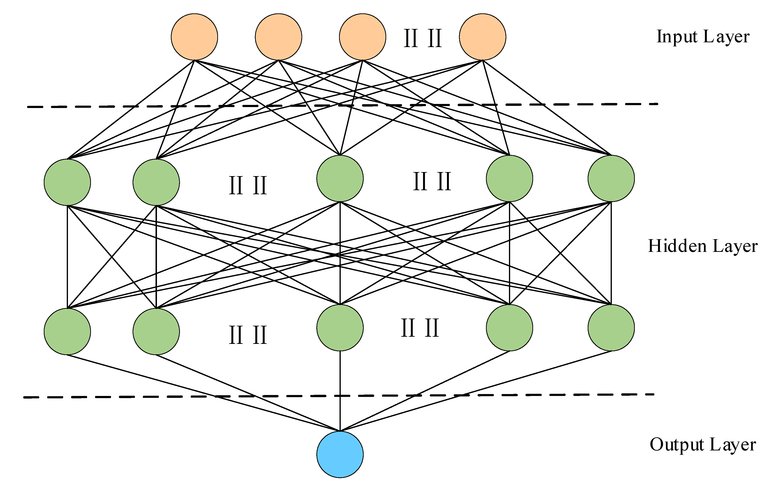
3.2. Basic Principles of LSTM

The traditional neural network model lacks the memory function of historical information, and the cyclic neural network (RNN) can apply the output information of previous neurons to the current task. However, conventional RNN has the problem of gradient disappearance or gradient explosion; in other words, when the time interval is large, the past learning results will disappear. To address these shortcomings, Hochreiter proposed the Long Short-Term Memory Neural Network (LSTM) in 1997. LSTM is a type of Recurrent Neural Network that can learn long-term dependent information. It not only has the memory function of historical information, but also overcomes the long-term dependence of the model and can selectively forget the invalid information and update the effective information, thus solving the problem of gradient dispersion to some extent. As shown in Figure 2, the LSTM network is composed of an input layer, an output layer and several recursive hiding layers between them. A recursive hiding layer is composed of multiple memory modules, each of which contains one or more self-connected memory units with three gates controlling the information flow: the input gate, the forgetting gate and the output gate. The state of LSTM cell is calculated as follows:
i t = σ ( W i × [ h t 1 , x t ] + b i )
f t = σ ( W f × [ h t 1 , x t ] + b f )
o t = σ ( W o × [ h t 1 , x t ] + b o )
c ˜ t = tanh ( W c × [ h t 1 , x t ] + b c )
c t = f t × c t 1 + i t × c ˜ t
In Equations (6)–(8), i t , f t and o t are, respectively, input gate, forgetting gate and output gate. In Equation (10), c t is a new candidate for cell state. LSTM cells act as state information, updating the c t of the old cell state c t 1 to the new cell state. W i , W f , W o and W c are, respectively, the weights of input, forgetting, output and current cell state. b i , b f , b o and b c are, respectively, the deviations of input, forgetting, output and current cell state.

4. Empirical Study

4.1. Data Description and Preprocessing

This paper selects four macroeconomic indicators of Gross Domestic Product (GDP), Consumer Price Index (CPI), Industrial Added Value (IAV) and Total Imports and Exports (TIE), as well as two related power generation indicators of National Total Power Generation (NTPG) and Hydropower Generation (HG), as input variables. To accurately evaluate the accuracy of wind power generation prediction model, this paper selects macroeconomic indicators and related power generation indicators from the National Bureau of Statistics of China. Macroeconomic indicators and related power generation data from the third quarter of 2009 to the second quarter of 2019 are selected, with a total of 40 data points. The original data samples are divided into two datasets: 80% of the original data (32 data points) are used as training samples and the remaining 20% (8 data points) are used as test samples to evaluate the predictive performance of the model.
Since the macroeconomic indicators and related power generation indicators have different dimensions and dimensional units, it is necessary to carry out data standardization processing for the original time series in order to eliminate the dimensional impact between indicators. According to Equation (11), each group of data is normalized into the interval 0–1 to solve the comparability between indicators, reduce the influence of outliers and noise and speed up the training speed of the model.
x i * = x i x min x max x min
The Matrix Laboratory (MATLAB) wavelet toolbox is used to decompose the normalized time series s ( t ) ; then,
s ( t ) = a J ( t ) + r = 1 3 d r ( t )
where J is the decomposition scale, a J ( t ) is the low-frequency component close to the original sequence, d r ( t ) is the detail signal component (high-frequency component) of the r -th decomposition and t is the discrete time.

4.2. Model Parameters

In this paper, the time series of multiple macroeconomic indicators and related power generation indicators after WD are taken as the input variables LSTM neural network, and the wind power generation of the whole country is taken as the output variable. The LSTM neural network contains four parameters that affect the prediction accuracy of the model, including the time step of each layer in the LSTM neural network, the number of hidden units in each layer in the model and the training times. In the process of training the model, the other parameters are the same each time, but the single parameter is different, so as to find the best prediction model. Each parameter setting in the model is shown in Table 1.
The LSTM model is a deep learning neural network, which has three layers: an input layer, a hidden layer and an output layer. The input is composed of six input variables: Gross Domestic Product (GDP), Consumer Price Index (CPI), Industrial Added Value (IAV), Total Imports and Exports (TIE), National Total Power Generation (NTPG) and Hydropower Generation (HG). The hidden layer consists of two LSTM units with time steps of 2, and each LSTM unit contains 64 cells. The output layer contains an output variable of wind power generation. The structure of the LSTM model is shown in Figure 3.

4.3. Performance Indicators

To further verify the effectiveness and performance of the prediction method proposed for wind power prediction, three error analysis criteria are introduced to evaluate the proposed model, as given in Equations (13)–(15) (where y _ r e a l i is the actual values and y _ p r e d i is predicted values). The mean absolute error (MAE), root mean square error (RMSE) and mean absolute percentage error (MAPE) are used to evaluate the performance of each method.
MAE = 1 N i = 1 N | y _ r e a l i y _ p r e d i |
MAPE = 1 N i = 1 N | y _ r e a l i y _ p r e d i y _ r e a l i | * 100
RMSE = i = 1 N ( y _ r e a l i y _ p r e d i ) 2 N

5. Results and Analysis
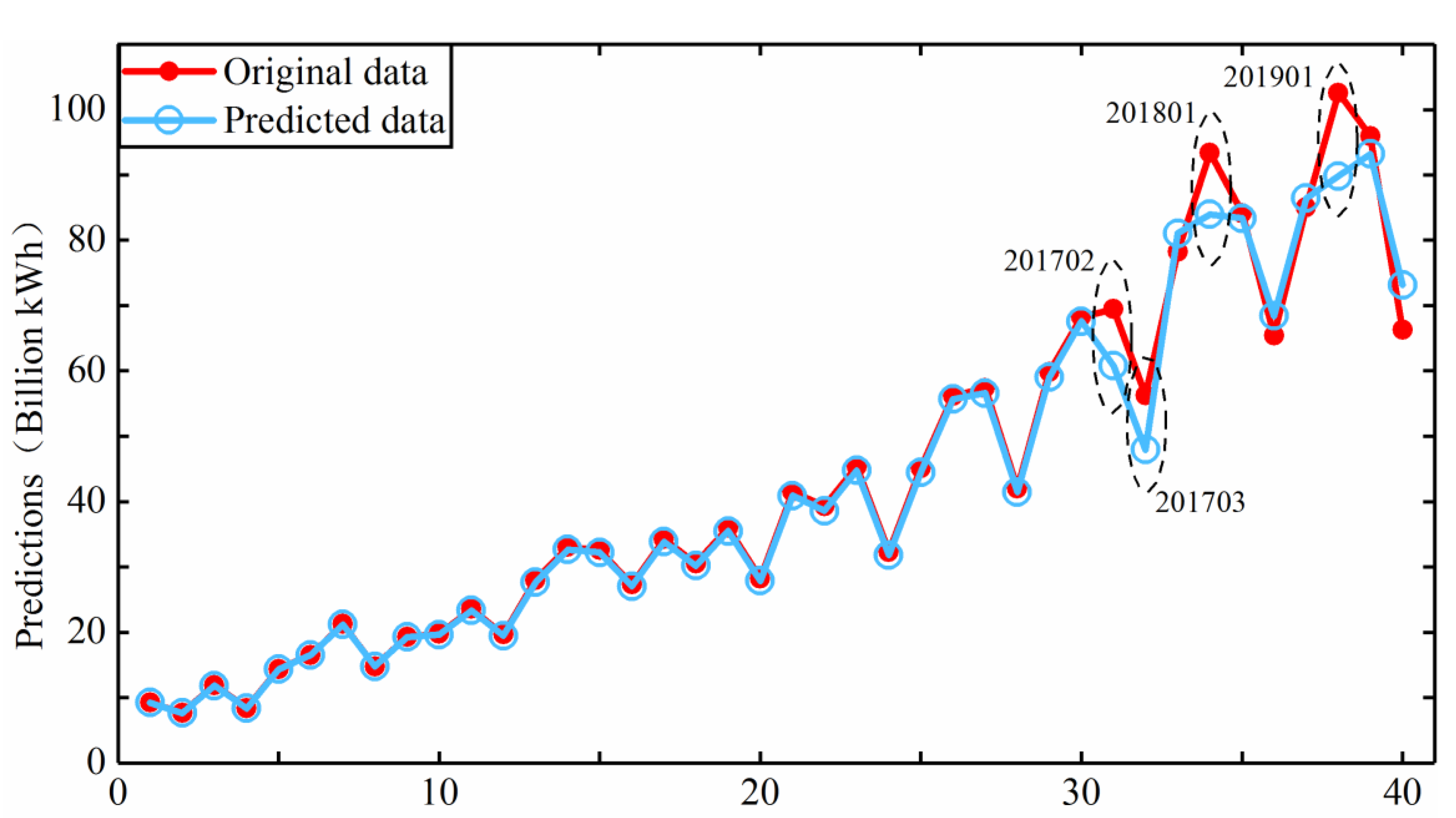
5.1. Model Accuracy

To evaluate the performance of WD-LSTM model in wind power prediction more effectively, other models are preliminarily selected for comparison in the paper. The physical or statistical models commonly used to predict by time series are selected. In addition, the models commonly used in machine learning and deep learning are selected. Bayesian Model Averaging and Ensemble Learning (BMA-EL) proposed by Wang et al. can accurately predict wind power generation under different meteorological conditions. Chen et al. built Multi-Resolution Multi-Learner Ensemble and Adaptive Model Selection (MRMLE-AMS), which presented high accuracy in wind power prediction by time series. Li et al. proposed the Support Vector Machine and Improved Dragonfly Algorithm model (SVR-IDA). In this paper, these models are selected as the comparison object for experimental verification. The results are shown in Table 2.
As shown in Table 2, among the four models, the MAPE of WD-LSTM model is the lowest, reaching 5.831. The MAPE of SVR-IDA model comes in second at 15.679, more than 10. The errors of BMA-EL and MRMLE-AMS are relatively high, exceeding 20. In this experiment, the accuracy of machine learning and deep learning prediction models is generally better than that of physical or statistical prediction models. The presumed reason may be that machine learning and deep learning predictive models can fully learn the correlation between input and output variables, similar to human neural networks. In particular, the deep learning model can more fully learn the variation trend of data in time series, hence showing a higher prediction accuracy.
Based on previous comparisons, the prediction model proposed in this paper, which combines wavelet decomposition with long short-term memory neural network, has shown high prediction accuracy when predicting wind power generation in China. To effectively evaluate the performance of WD-LSTM in wind power prediction, traditional prediction methods of machine learning and deep learning are used in this paper as comparative experiments. Based on the same input time series, the learning situation of each model is tested, and its errors are compared and analyzed. During the experiment, Support Vector Regression (SVR), Gate Recurrent Unit (GRU), Wavelet Decomposition and Support Vector Regression (WD-SVR) and Wavelet Decomposition and Gated Recurrent Unit (WD-GRU) are used for time series prediction as comparative tests. In addition, the proportion of training set and test set is the same as that of WD-LSTM model and five comparative experiments are conducted. To objectively evaluate and describe the performance of the six prediction models, the prediction error values of each model are calculated according to the above formulas. The experimental results of MAE, MAPE and RMSE of the raw test set are shown in Table 3.
Among all the experimental models, WD-SVR has the largest error, and its MAE, MAPE and RMSE are 206.831, 20.153 and 212.016, respectively. The MAE, MAPE and RMSE of WD-GRU are 144.321, 18.034 and 226.302, respectively. The MAPE of the three models of SVR, GRU and LSTM are similar, 15.351, 15.048 and 13.715, respectively. The error of WD-LSTM model is the smallest, and its MAPE is 5.831, which is significantly lower than the other five models. It can be seen from the data in Table 3 that WD-LSTM has a high accuracy in predicting wind power generation and is more effective than the traditional models and single models. Furthermore, Table 3 shows computing time cost of WD-LSTM and five other comparison models. In the machine learning models, the prediction using SVR model took 0.05 min while WD-LSTM took 12.05 min. In the deep learning models, GRU and LSTM cost the same time, 32 min, while WD-GRU and WD-LSTM cost the same time, 44 min. In general, compared with machine learning models, deep learning models take a longer time to predicate using time series. However, as for deep learning models, since the data samples are relatively small, there is no significant difference in the time spent on prediction.
Figure 4 shows the prediction results of WD-LSTM neural network and five other comparison models, which directly reflects the degree of fitting between the predicted values of the six models and the real values. Meanwhile, Figure 5 shows the predicted and original value based on WD-LSTM. As shown in Figure 4, the prediction curve of Support Vector Regression (SVR) is relatively stable and it is difficult to predict the dynamic change of data. When the data present a large fluctuation, the model presents a large error value. Gated Recurrent Unit (GRU) is a variant or simplification of the Long Short-Term Memory network (LSTM), which includes reset gate and update gate. From the forecast results, it can reflect the fluctuation of wind power generation, but the variation trend in a single quarter is opposite to the real value, leading to higher error value. The results show that the input indexes such as Gross Domestic Product (GDP), Consumer Price Index (CPI), Industrial Added Value (IAV), Total Imports and Exports (TIE), National Total Power Generation (NTPG) and Hydropower Generation (HG) can be used as the input data of wind power generation. WD-LSTM can accurately predict the fluctuation of wind power generation, and the error value is lower than other models.
On the basis of the above research, the paper further studies the influence of different types of input indicators on the accuracy of wind power generation prediction. The six input indicators are divided into two categories: (1) macroeconomic indicators, including GDP, CPI, IAV and TIE; and (2) power generation indicators, including NTPG and HG. The two kinds of indicators are, respectively, taken as input variables, and the WD-LSTM model is used to predict wind power generation on the condition that the model parameters are kept consistent. When macroeconomic indicators are taken as input variables, the experimental result of MAPE is 19.732. When the related power generation index is used as the input variables, the MAPE is 16.298. The results show that wind power forecast achieves the best prediction accuracy when six indicators are used as input variables.

5.2. Sensitivity Analysis

Sensitivity analysis is a common method to study and analyze the effect of parameter changes on system behavior. The sensitivity of variables to test parameters can be calculated as follows:
s t = | ( Y t Y t ) / Y t ( X t X t ) / X t |
where S t is the sensitivity of variables to test parameters at time t , setting the third quarter of 2009 as t = 1 ; Y t and Y t are the value of output variable before and after change at time t ; and X t and X t are the value of input variables before and after change at time t. The maximum sensitivity of wind power generation during 2006–2017 is:
s = m a x ( S t ) , 1 t 40
The sensitivity of the wind power generation variable on the six main input variable in the proposed WD-LSTM model is studied and analyzed by changing the corresponding input variables by −5%, −3%, −1%, 1%, 3% and 5%, and the maximum sensitivity of wind power generation from the third quarter of 2009 to the second quarter of 2019 with respect to the six input variables change is shown in Table 4.
It is found that the maximum sensitivity of wind power generation in the proposed model with respect to the six input variables from the third quarter of 2009 to the second quarter of 2019 is less than 0.10, which means the maximum sensitivity of wind power generation in the proposed WD-LSTM model is less sensitive. Therefore, the proposed model is stable and does not cause abnormal fluctuations in the output variable data due to the small changes of input variables.

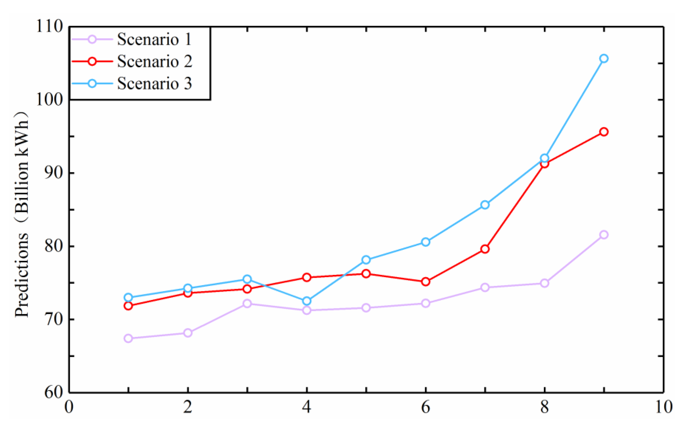
5.3. Scenarios Setting

Different scenarios for forecasting are set in this paper, in which different scenarios match different input data to explore the changing trend of national wind power generation under different development situations and reduce the uncertainty of forecasting. Taking historical data rates and national economic, energy and social macro-development plans into account to make more realistic predictions and analyze the future trends of each characteristic value, this paper sets the following three scenarios to predict the wind power generation in China under different development trends in the next two years. Scenario 1 is a low-growth scenario, which keeps the country’s recent development trend sustainable and calculates the minimum growth rate (non-negative) of macroeconomic indicators and related power generation indicators based on the growth rate of historical data to predict the national wind power generation. Scenario 2 is the base scenario, in which the development trend of each indicator is predicted more accurately and in line with the actual development trend from the fourth quarter of 2019 to the fourth quarter of 2022, and the average year-on-year growth rate of the data from the third quarter of 2009 to the second quarter of 2019 is calculated. Scenario 3 is a high-growth scenario, which maintains a high growth rate according to the historical development trend. According to the data from the third quarter of 2009 to the second quarter of 2019, the average year-on-year growth rate of each quarter is calculated and increased by 1.2 times on the basis of the average growth rate of each quarter. The specific growth rates under each scenario are shown in Table 5.

5.4. Future Prediction Results

By comparing the error values of each single model and the hybrid model in the prediction of wind power generation across the country through testing, we obtained that the prediction accuracy of WD-LSTM is relatively high, and predicted the wind power generation of China in the next two years by this model (from the fourth quarter of 2019 to the fourth quarter of 2021). The index data of different growth trends are substituted into WD-LSTM for the prediction of wind power generation in China based on the above scenario settings, and the prediction results under three different scenarios are compared, as shown in Figure 6. Wind power generation is projected to grow at a slower pace in Scenario 1, from 66.3 billion kWh in the third quarter of 2019 to 81.6 billion kWh in the fourth quarter of 2021, an increase of 15.3 billion kWh over nine quarters. Wind power generation forecasting show an increase in Scenario 2 from 66.3 billion kWh in the third quarter of 2019 to 95.6 billion kWh in the fourth quarter of 2021, an increase of 29.4 billion kWh in nine quarters. Scenario 3 is of high growth, from 66.3 billion kWh in the third quarter of 2019 to 105.6 billion kWh in the fourth quarter of 2021, an increase of 39.4 billion kWh in nine quarters. In summary, the forecast results of the three scenarios show that the total national wind power output will fluctuate between 283.1 and 300.4 billion kWh in 2020, and the total national wind power output will be between 303.1 and 363.9 billion kWh in 2021, floating from time to time.
From the overall trend, the country’s wind power generation will continue to increase. Under the three scenarios, the national wind power generation will decline slightly in the first quarter of 2020, and the growth rate will peak in the fourth quarter of 2021. In 2017, the State Grid pointed out at a press conference that, by 2020, the problem of new energy consumption will be completely solved, and the rate of abandoned wind and light will be controlled within 5%. According to the 13th Five-Year Plan for Wind Power Development, by 2020, non-fossil energy will account for 15% of primary energy consumption, and the country’s annual wind power generation will need to reach 42 billion kWh and 6% of the total power generation. The sustained growth of wind power generation in China in the future may be affected by the following factors: (1) The sustained and steady development of China’s economy. At the present stage, China’s economic development model is changing from high-speed development to high-quality development. The steady high-quality economic development has laid a solid foundation for the development of the wind power industry in China, thus realizing the sustainable growth of the country’s wind power generation. (2) Environmental protection brings development opportunities for renewable energy such as wind energy. From the overall perspectives, the development of renewable energy is a common goal of mankind and an important support for the global response to future climate, environmental and economic changes. The development of wind power as an energy source can become more affordable than traditional coal power, and the parity of wind power will release new market space, which is also an important reason for the continuous growth of wind power generation across the country.
Wind power in China shows a trend of rapid development. Wind curtailment and power limiting has become the focus of society and a major problem that needs to be solved urgently in power grid planning and dispatching operation. In 2017, the National Energy Administration’s Guidance on the Implementation of the 13th Five-Year Plan for the Development of Renewable Energy was released. At the same time, the target of consumption and utilization is also proposed to effectively solve the problem of wind power curtailment by 2020. From 2011 to 2016, the wind curtailment rate showed a trend of first decreasing and then increasing, reaching the highest value of 17.1% in 2016. According to the Clean Energy Consumption Action Plan (2018–2020) jointly issued by the National Development and Reform Commission and the National Energy Administration, the wind curtailment rate will be kept at a reasonable level (aiming at around 5%) by 2020. Based on previous predictions, the total national wind power output will fluctuate between 283.1 and 300.4 billion kWh in 2020. Consequently, wind curtailment power will keep between 14.1 and 15.0 billion kWh in 2020.

6. Conclusions

As a kind of renewable energy, wind power generation plays a crucial role in China’s electric energy production. Therefore, accurate prediction of wind power generation is helpful to optimize the power grid dispatching, reduce the reserve capacity of the system and reduce the operating cost of the power system. In this paper, a hybrid LSTM model for predicting wind power generation in China is constructed based on six index factors: gross domestic product, consumer price index, industrial added value, total imports and exports, total power generation and hydropower generation. Based on wavelet decomposition and long short-term memory neural network methods, a hybrid WD-LSTM model for predicting national wind power generation is constructed. The following conclusions can be reached through experiments:
(1)
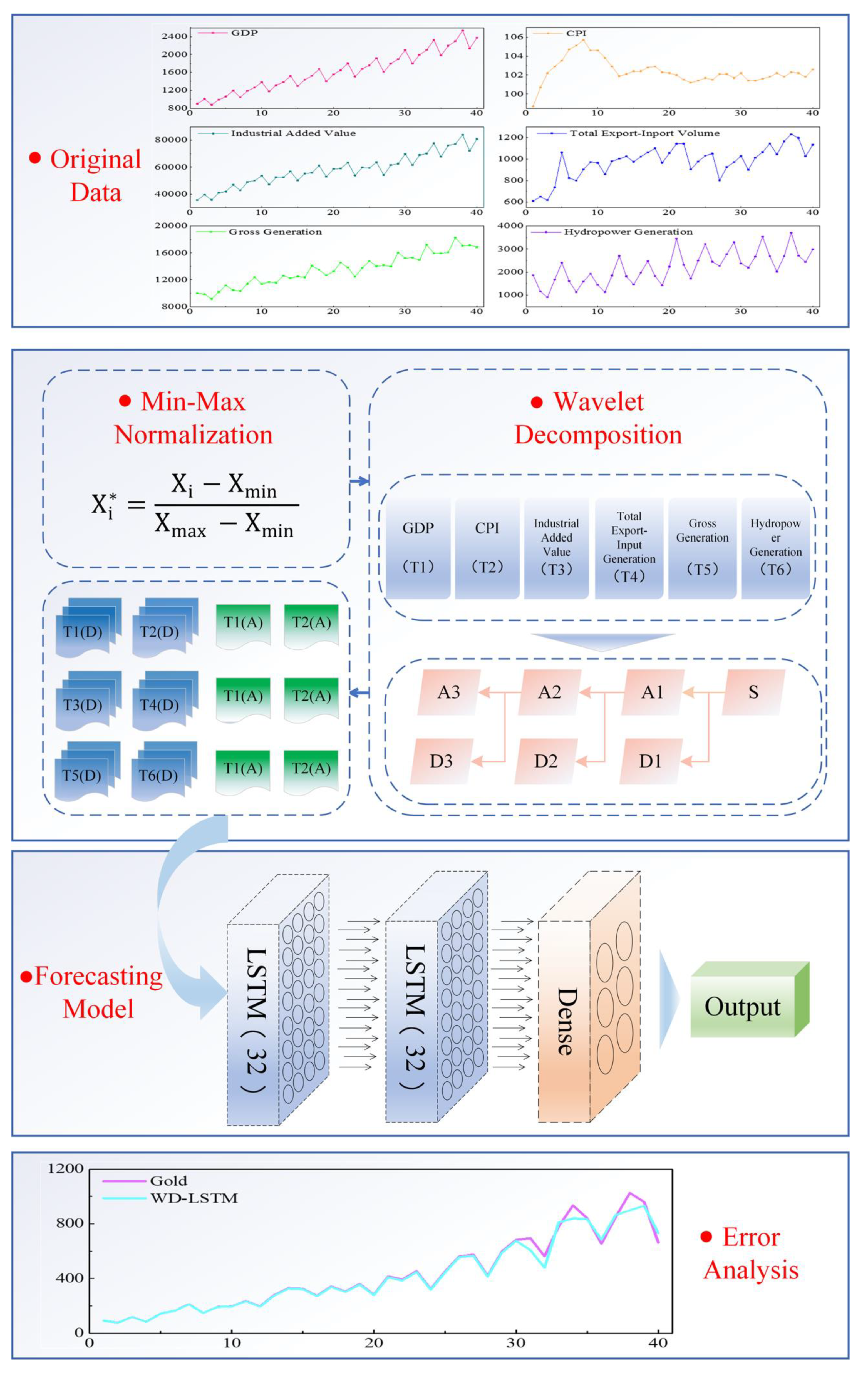
Wind power generation is related to GDP, CPI, IAV, TIE, TPG and HG. The selection of these six input indexes can, to a certain extent, predict the wind power generation of the country.
(2)
The time series of macroeconomic indicators and related power generation indicators are decomposed into low-frequency components and high-frequency components through wavelet decomposition, which increases the data dimension of the input variables of the prediction model to some extent. The time series data of macroeconomic and related power generation indexes of different frequencies are used as input variables to effectively improve the accuracy of the prediction model.
(3)
In this paper, the WD-LSTM hybrid prediction model is selected to predict the wind power generation in China. The experimental results show that the MAPE of the mixed prediction model is 5.831. Compared with machine learning and a single prediction model, the model can predict wind power generation more accurately across the country.
(4)
In addition, the prediction of national wind power generation in this paper still needs to be improved and deepened. Due to the difficulty in obtaining some index data and the inconsistency of some data in scale, the paper has the limitation in the selection of input indices. The limitations of the samples themselves will lead to a certain range of errors in the process of data processing and prediction. Therefore, other possible influencing factors can be considered as input variables.
(5)
The next step of the study will consider whether the time series with different scales can be used as the input index of the same model. At the same time, Information Gain (IG) will also be used to sort and filter input indicators by correlation, and then make prediction using WD-LSTM model. The application of the proposed model in primary energy consumption or renewable energy consumption will also be considered.

Author Contributions

Data curation, S.Z., X.Y. and L.Z.; Formal analysis, S.Z.; Investigation, X.Y. and L.Z.; Methodology, B.L.; Software, Q.W.; Supervision, B.L.; Writing—original draft, S.Z.; and Writing—review and editing, B.L. and Q.W. All authors have read and agreed to the published version of the manuscript.

Funding

This research was funded by the National Natural Science Foundation of China (grant number 71503180) and Humanities and Social Sciences Fund of the Ministry of Education (grant number 20YJA630042).

Conflicts of Interest

The authors declare no conflict of interest.

References

  1. Wuyong, Q.; Jue, W. An improved seasonal GM (1,1) model based on the HP filter for forecasting wind power generation in China. Energy 2020, 209, 118499. [Google Scholar]
  2. Xu, X.; Niu, D.; Xiao, B.; Guo, X.; Zhang, L.; Wang, K. Policy analysis for grid parity of wind power generation in China. Energy Policy 2020, 138, 111225. [Google Scholar] [CrossRef]
  3. Messner, J.W.; Pinson, P. Online adaptive lasso estimation in vector autoregressive models for high dimensional wind power forecasting. Int. J. Forecast. 2019, 35, 1485–1498. [Google Scholar] [CrossRef]
  4. Han, S.; Qiao, Y.-H.; Yan, J.; Liu, Y.-Q.; Li, L.; Wang, Z. Mid-to-long term wind and photovoltaic power generation prediction based on copula function and long short term memory network. Appl. Energy 2019, 239, 181–191. [Google Scholar] [CrossRef]
  5. Wang, Y.; Liu, Y.; Li, L.; Infield, D.; Han, S. Short-Term Wind Power Forecasting Based on Clustering Pre-Calculated CFD Method. Energies 2018, 11, 854. [Google Scholar] [CrossRef] [Green Version]
  6. Natapol, K.; Thananchai, L. Robust short-term prediction of wind power generation under uncertainty via statistical interpretation of multiple forecasting models. Energy 2019, 180, 387–397. [Google Scholar]
  7. Shao, H.; Deng, X.; Jiang, Y. A novel deep learning approach for short-term wind power forecasting based on infinite feature selection and recurrent neural network. J. Renew. Sustain. Energy 2018, 10, 043303. [Google Scholar] [CrossRef]
  8. Wang, H.; Lei, Z.; Wu, Q.H.; Peng, J.; Liu, J. Echo state network based ensemble approach for wind power forecasting. Energy Convers. Manag. 2019, 201, 112188. [Google Scholar] [CrossRef]
  9. Wang, G.; Jia, R.; Liu, J.; Zhang, H. A hybrid wind power forecasting approach based on Bayesian model averaging and ensemble learning. Renew. Energy 2020, 145, 2426–2434. [Google Scholar] [CrossRef]
  10. Wang, C.; Zhang, H.; Ma, P. Wind power forecasting based on singular spectrum analysis and a new hybrid Laguerre neural network. Appl. Energy 2020, 259, 114139. [Google Scholar] [CrossRef]
  11. Wang, H.; Han, S.; Liu, Y.; Yan, J.; Li, L. Sequence transfer correction algorithm for numerical weather prediction wind speed and its application in a wind power forecasting system. Appl. Energy 2019, 237, 1–10. [Google Scholar] [CrossRef]
  12. Pearre, N.S.; Swan, L.G. Statistical approach for improved wind speed forecasting for wind power production. Sustain. Energy Technol. Assess. 2018, 27, 180–191. [Google Scholar] [CrossRef]
  13. Leng, H.; Li, X.; Zhu, J.; Tang, H.; Zhang, Z.; Ghadimi, N. A new wind power prediction method based on ridgelet transforms, hybrid feature selection and closed-loop forecasting. Adv. Eng. Inform. 2018, 36, 20–30. [Google Scholar] [CrossRef]
  14. Wang, K.; Qi, X.; Liu, H.; Song, J. Deep belief network based k-means cluster approach for short-term wind power forecasting. Energy 2018, 165, 840–852. [Google Scholar] [CrossRef]
  15. Semero, Y.K.; Zhang, J.; Zheng, D.; Wei, D. A GA-PSO Hybrid Algorithm Based Neural Network Modeling Technique for Short-term Wind Power Forecasting. Distrib. Gener. Altern. Energy J. 2018, 33, 26–43. [Google Scholar] [CrossRef]
  16. Hong, D.; Ji, T.; Li, M.; Wu, Q. Ultra-short-term forecast of wind speed and wind power based on morphological high frequency filter and double similarity search algorithm. Int. J. Electr. Power Energy Syst. 2019, 104, 868–879. [Google Scholar] [CrossRef]
  17. Du, P.; Wang, J.; Yang, W.; Niu, T. A novel hybrid model for short-term wind power forecasting. Appl. Soft Comput. 2019, 80, 93–106. [Google Scholar] [CrossRef]
  18. Lu, P.; Ye, L.; Sun, B.; Zhang, C.; Zhao, Y.; Teng, J. A New Hybrid Prediction Method of Ultra-Short-Term Wind Power Forecasting Based on EEMD-PE and LSSVM Optimized by the GSA. Energies 2018, 11, 697. [Google Scholar] [CrossRef] [Green Version]
  19. Yagang, Z.; Yuan, Z.; Chunhui, K.; Bing, C. A new prediction method based on VMD-PRBF-ARMA-E model considering wind speed characteristic. Energy Convers. Manag. 2020, 203, 112254. [Google Scholar]
  20. Naik, J.; Satapathy, P.; Dash, P. Short-term wind speed and wind power prediction using hybrid empirical mode decomposition and kernel ridge regression. Appl. Soft Comput. 2018, 70, 1167–1188. [Google Scholar] [CrossRef]
  21. Wang, C.; Zhang, H.; Fan, W.; Ma, P. A new chaotic time series hybrid prediction method of wind power based on EEMD-SE and full-parameters continued fraction. Energy 2017, 138, 977–990. [Google Scholar] [CrossRef]
  22. Wang, K.; Niu, D.; Sun, L.; Zhen, H.; Liu, J.; De, G.; Xu, X. Wind Power Short-Term Forecasting Hybrid Model Based on CEEMD-SE Method. Processes 2019, 7, 843. [Google Scholar] [CrossRef] [Green Version]
  23. Han, L.; Zhang, R.; Wang, X.; Bao, A.; Jing, H. Multi-step wind power forecast based on VMD-LSTM. IET Renew. Power Gener. 2019, 13, 1690–1700. [Google Scholar] [CrossRef]
  24. Cavalcante, L.; Bessa, R.; Reis, M.; Browell, J. LASSO vector autoregression structures for very short-term wind power forecasting. Wind. Energy 2016, 20, 657–675. [Google Scholar] [CrossRef] [Green Version]
  25. Wang, Y.; Hu, Q.; Meng, D.; Zhu, P. Deterministic and probabilistic wind power forecasting using a variational Bayesian-based adaptive robust multi-kernel regression model. Appl. Energy 2017, 208, 1097–1112. [Google Scholar] [CrossRef]
  26. Chen, C.; Liu, H. Medium-term wind power forecasting based on multi-resolution multi-learner ensemble and adaptive model selection. Energy Convers. Manag. 2020, 206, 112492. [Google Scholar] [CrossRef]
  27. Ouyang, T.; Huang, H.; He, Y.; Tang, Z. Chaotic wind power time series prediction via switching data-driven modes. Renew. Energy 2020, 145, 270–281. [Google Scholar] [CrossRef]
  28. Liu, M.; Cao, Z.; Zhang, J.; Wang, L.; Huang, C.; Luo, X. Short-term wind speed forecasting based on the Jaya-SVM model. Int. Jelec Power 2020, 121, 106056. [Google Scholar] [CrossRef]
  29. Zhang, Y.; Le, J.; Liao, X.; Zheng, F.; Li, Y. A novel combination forecasting model for wind power integrating least square support vector machine, deep belief network, singular spectrum analysis and locality-sensitive hashing. Energy 2019, 168, 558–572. [Google Scholar] [CrossRef]
  30. Nielson, J.; Bhaganagar, K.; Meka, R.; Alaeddini, A. Using atmospheric inputs for Artificial Neural Networks to improve wind turbine power prediction. Energy 2020, 190, 116273. [Google Scholar] [CrossRef]
  31. Qin, Y.; Li, K.; Liang, Z.; Lee, B.; Zhang, F.; Gu, Y.; Zhang, L.; Wu, F.; Rodriguez, D. Hybrid forecasting model based on long short term memory network and deep learning neural network for wind signal. Appl. Energy 2019, 236, 262–272. [Google Scholar] [CrossRef]
  32. Li, L.; Zhao, X.; Tseng, M.-L.; Tan, R. Short-term wind power forecasting based on support vector machine with improved dragonfly algorithm. J. Clean. Prod. 2020, 242, 118447. [Google Scholar] [CrossRef]
  33. Yuan, X.; Chen, C.; Jiang, M.; Yuan, Y. Prediction interval of wind power using parameter optimized Beta distribution based LSTM model. Appl. Soft Comput. 2019, 82, 105550. [Google Scholar] [CrossRef]
  34. Lu, K.; Sun, W.X.; Wang, X.; Meng, X.R.; Zhai, Y.; Li, H.H.; Zhang, R.G. Short-term Wind Power Prediction Model Based on Encoder-Decoder LSTM. IOP Conf. Series: Earth Environ. Sci. 2018, 186, 012020. [Google Scholar] [CrossRef]
  35. López, E.; Valle, C.; Allende, H.; Gil, E.; Madsen, H. Wind Power Forecasting Based on Echo State Networks and Long Short-Term Memory. Energies 2018, 11, 526. [Google Scholar] [CrossRef] [Green Version]
  36. Jinhua, Z.; Yan, J.; Infield, D.; Liu, Y.; Lien, F.-S. Short-term forecasting and uncertainty analysis of wind turbine power based on long short-term memory network and Gaussian mixture model. Appl. Energy 2019, 241, 229–244. [Google Scholar] [CrossRef] [Green Version]
  37. Han, L.; Jing, H.; Zhang, R.; Gao, Z. Wind power forecast based on improved Long Short Term Memory network. Energy 2019, 189, 116300. [Google Scholar] [CrossRef]
  38. Naik, J.; Dash, S.; Dash, P.; Bisoi, R. Short term wind power forecasting using hybrid variational mode decomposition and multi-kernel regularized pseudo inverse neural network. Renew. Energy 2018, 118, 180–212. [Google Scholar] [CrossRef]
  39. Yu, R.; Gao, J.; Yu, M.; Lu, W.; Xu, T.; Zhao, M.; Zhang, J.; Zhang, R.; Zhang, Z. LSTM-EFG for wind power forecasting based on sequential correlation features. Futur. Gener. Comput. Syst. 2019, 93, 33–42. [Google Scholar] [CrossRef]
  40. Lin, Z.; Liu, X.; Collu, M. Wind power prediction based on high-frequency SCADA data along with isolation forest and deep learning neural networks. Int. J. Electr. Power Energy Syst. 2020, 118, 105835. [Google Scholar] [CrossRef]
  41. Akira, R.; Hiroka, R. Application of multi-dimensional wavelet transform to fluid mechanics. Theor. Appl. Mech. Lett. 2020, 10, 98–115. [Google Scholar]
Figure 1. Calculation process of the WD-LSTM model.
Energies 13 04964 g001
Figure 2. Schematic diagram of neurons.
Energies 13 04964 g002
Figure 3. The structure of LSTM neural network.
Energies 13 04964 g003
Figure 4. Forecasting performance of the WD-LSTM model and five other models.
Energies 13 04964 g004
Figure 5. Forecasting results of wind power generation based on WD-LSTM model.
Energies 13 04964 g005
Figure 6. Predictions for wind power generation in different scenarios.
Energies 13 04964 g006
Table 1. Parameters for the LSTM network.
DatasetTime StepsHidden LayersBatch SizeLrEpoch
WD-LSTM26430.00115,000
Table 2. Comparison of forecasting errors using different models.
AlgorithmsBMA-ELMRMLE-AMSSVR-IDAWD-LSTM
MAPE22.32820.62415.6795.831
Table 3. Comparison of prediction performances using machine learning and deep learning models.
AlgorithmsMAEMAPERMSEComputing Time
(Minutes)
SVR137.88815.351 165.175 0.05
GRU127.86315.048 177.223 32
LSTM101.51113.715 169.644 32
WD-SVR206.83120.153212.01612.05
WD-GRU144.32118.034226.30244
WD-LSTM49.8965.831 63.991 44
Table 4. The maximum sensitivity of wind power generation with respect to the six variables.
Input VariablesChange Rate
−5%−3%−1%1%3%5%
Gross Domestic Product (GDP)0.096350.094750.095200.095200.094550.09635
Consumer Price Index (CPI)0.006150.006050.006750.006750.005950.00615
Industrial Value Added (IVA)0.070870.069130.070000.070000.069130.07087
Total Imports and Exports (TIE)0.048300.048850.047150.047150.048850.04830
Total Power Generation (TPG)0.059100.068750.060450.060450.063700.05910
Hydroelectricity Generation (HG)0.005230.004670.004800.004800.004670.00523
Table 5. Growth rates in different scenarios.
Different
Scenarios
Gross Domestic Product
(GDP)
Consumer Price Index
(CPI)
Industrial Value Added
(IVA)
Total Imports and Exports
(TIE)
Total Power Generation
(TPG)
Hydroelectricity Generation
(HG)
Scenario 12.6220.0970.7740.0530.3065.739
Scenario 23.1460.1012.6452.3451.6036.455
Scenario 33.7750.1223.1742.8151.9247.746

