Least Squares Method for Identification of IGBT Thermal Impedance Networks Using Direct Temperature Measurements

Abstract

State-of-the-art methods for determining thermal impedance networks for IGBT (Insulated Gate Bipolar Transistor) modules usually involves the establishment of the relationship between the measured transistor or diode voltage and temperature under homogenous temperature distribution across the IGBT module. The junction temperature is recomputed from the established voltage–temperature relationship and used in determining the thermal impedance network. This method requires accurate measurement of voltage drop across the transistors and diodes under specific designed heating and cooling profiles. Validation of the junction temperature is usually done using infrared camera or sensors placed close to the transistors or diodes (in some cases and open IGBT module) so that the measured temperature is as close to the junction as possible. In this paper, we propose an alternative method for determining the IGBT thermal impedance network using the principles of least squares. This method uses measured temperatures for defined heating and cooling cycles under different cooling conditions to determine the thermal impedance network. The results from the proposed method are compared with those obtained using state-of-the-art methods.

1. Introduction

Operation of inverters under peak load and frequent thermal transient conditions requires a precise estimation of the junction temperature for effective thermal management. These conditions are common in inverters used in automotive traction drives operating under low speed and high torque demands such as stop-and-go situations in city driving, off-road/uphill driving, or towing a trailer. In some cases, IGBT modules are equipped with temperature sensors. Typical sensors used usually have a slow thermal response [1,2] and are much more suitable for measuring baseplate or case temperatures with high thermal time constants compared to the junction temperature. Even if much more accurate sensors or those with faster responses were to be used, a sensor will have to be placed close to each diode or transistor in the IGBT module. During asymmetrical loading of the inverter, some transistors or diodes allow higher currents than others and consequently have higher temperatures. Hence, depiction of individual diodes and transistor temperatures is necessary [3]. Placing sensors close to each transistor or diode in an IGBT module increases the overall cost of the inverter and also presents some packaging challenges. In addition to effective real-time thermal management and control of inverters [4], information about the junction temperature is imperative in the study of ageing and degradation of IGBT modules [5,6,7,8,9]. Such studies provide vital information needed in implementing appropriate thermal management and control strategies of the inverter which limit frequent operation of the inverter in thermally critical temperature ranges, thereby extending the lifetime of the IGBT module and consequently in overall lifetime of the inverter [10,11,12,13].

Junction temperature estimation typically stems from a model of the electro-thermal behaviour of the IGBT module. Typical models can be expressed as RC circuits where resistances and capacitances represent the thermal impedances and capacitances of the individual elements (transistors and diodes) of the module. These RC circuits describe the heat transfer between the heat source and the heat sink. Two types of RC-circuit thermal networks are most frequently used in thermal modelling of an IGBT module: Foster network [3,14,15] and Cauer network [16,17]. Thermal impedances of RC thermal networks can be determined using finite element methods [18,19,20], VCE (collector–emitter voltage) measurement methods (thermo-sensitive electrical parameter—TSEP) [21,22,23,24,25], or direct temperature measurements using sensors [21,26]. Finite element methods are suitable in the determination of parameters of both Cauer and Foster networks. Direct temperature measurement and TSEP methods are suitable in determining the Foster network parameters where only the junction temperature of the transistor or diode is important.

Finite element analysis (FEA) [27,28,29] provides detailed information about the thermal impedances between a heat source and a heat sink in an IGBT module. These models are usually based on ideal material properties and are very complex to implement. FEA models, though suited for extraction of thermal impedances, are not suited for online junction temperature estimation because of the high computational effort required [20]. Analytical junction estimation techniques [3,30,31,32,33] are widely used in industrial applications for online junction temperature estimation because it is not computationally intensive and thus suitable for implementation on microcontroller.

In [22], methods for determining thermal impedances from VCE based TSEP and direct temperature measurement were presented and validated using measurements from an infrared camera. In this paper, a similar experimental setup is used, but a novel method for extracting the thermal impedance parameters using the well-known least squares method is presented. This method takes advantage of the availability of development IGBT module with temperature sensors within close proximity to the transistor and diodes. These modules are used primarily in the validation of calculated junction temperatures. The novel least-squares-based approach eliminates the sources of error from the TSEP based VCE methods, which rely heavily on the accuracy of the measured voltages across the transistors and diodes as well as those measured temperatures in the cool-down phase.

The method presented is an analytical method and is well suited for implementation on a microcontroller. However, due to the limited computational power of microcontrollers used for mass production purposes, it is imperative to study the effect of the order of the thermal impedance network on the accuracy of the calculated junction temperature to obtain the optimal compromise between computational recourses and accuracy of the calculated junction temperature.

2. Direct Temperature Measurement

2.1. Experimental Setup

The experimental setup is as shown in Figure 1 below:

Eight temperature sensors (Figure 1b), type Pt100, numbered 1–8, are placed close to the transistors and diodes of the opened IGBT module so that the temperature measured in the steady state is comparable to the junction temperatures. The cooling fan (Figure 1d) attached to the heatsink on which the open IGBT module is mounted is used in varying the airflow rate so that temperature measurements are done under varying cooling conditions. The open IGBT module (Figure 1c) is sprayed with an emissivity spray to enhance measurement using the infrared camera (Figure 1a). The measured voltage, currents, and temperatures by the DSP (Figure 1b) are transferred to the laptop through a USB cable.

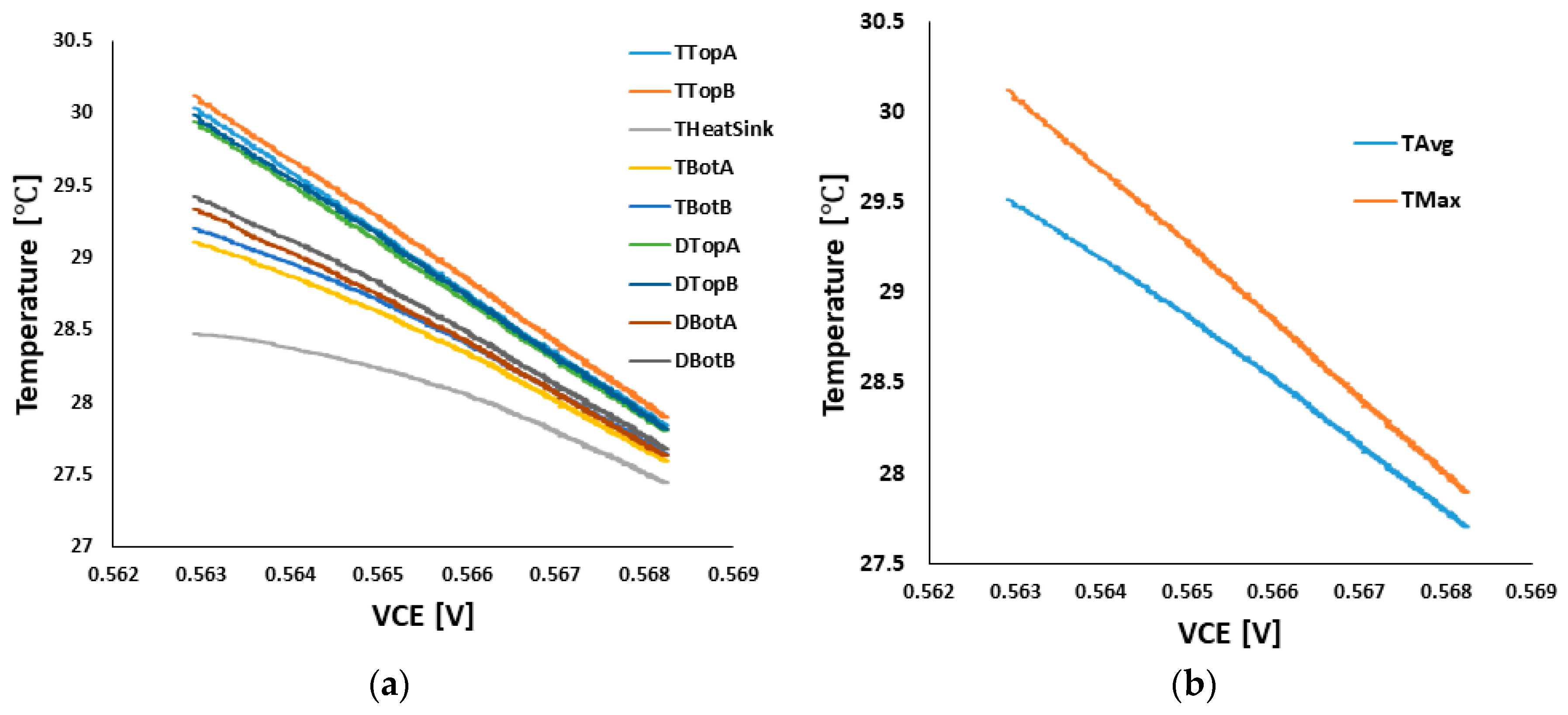
2.2. Voltage and Current Measurement

A current pulse of a defined duration is allowed through either the transistor or diode by closing switch S2 as shown in Figure 2. The corresponding temperatures of all transistors and diodes are measured for the entire heating and cooling cycle. Additionally, the voltage drop across the active IGBT or diode as well as the current is measured. The cooling fan is used in varying the air flowrate such that the experiment is done under varying cooling conditions. Due to the fact that the IGBT modules are opened, the maximum current through the transistors or diodes is limited to 50A. A typical measurement profile is shown in Figure 3.

Experimental data were collected for the following operating conditions indicated in

Table 1. Experimental data collection operating conditions.

Currents (A)	Air Flowrate (Meters per Second m/s)
25	0	0.5	1	5	14
50	0	0.5	1	5	14

.

Each element of the IGBT module (top diode, top transistor, bottom diode, bottom transistor) is operated individually under the conditions defined in Table 1, and its corresponding set of experimental data is recorded. These operating conditions are chosen to test the performance of the proposed model under different cooling conditions. Designation of the experimental data starts with the active element, followed by the air flowrate and the current. For example, Ttop_1mps25A is data collected for an active top transistor at current of 25A and 1 m per second cooling air flowrate.

3. Identification of Thermal Networks Using Least Squares

3.1. Linear Transfer Function

As an alternative to the conventional method, we study a linear multi-input, single-output representation of transfer function between the source of heat and the monitored temperature. For simplicity of notation, we present the model for a single element with temperature $T$, but it will be later used to model all elements. In discrete time, the temperature $T$ of the $m$th element evolves as

$$\begin{array}{rrr}\hfill T_{m,k}& \hfill =& \hfill {\displaystyle {\displaystyle \sum }_{i=1}^{\overline{i}}}\left({\displaystyle {\displaystyle \sum }_{l=1}^{\overline{l}}}\left(a_{m,l,i}{T}_{l,k-i}+z_{m,l,i}{P}_{l,k-i}\right)+c_{m,i}{T}_{\mathrm{bp},k-i}\right),\end{array}$$

(1)

where $k=1\dots \overline{k}$ is the index of the discrete time sample, $l=1\dots \overline{l}$ is the index of active element, $P_l$ is the instantaneous power input of the $l$th source, $l=1\dots ,\overline{l}.$ Index $i=1\dots \overline{i},$ denote delays in the temperatures and power inputs. The maximum delay of the data is $\overline{i}$, and the first measurement of the $l$th temperature that can be predicted by model (1) is ${\mathrm{T}}_{l,\overline{i}+1}$. Aggregating measurements in the full time series into vectors:

$$\begin{array}{rrr}\hfill T_{l,0}& =& {[T_{l,\overline{i}+1},\dots ,T_{\overline{k}}]}^{\top },\hfill \\ \hfill P_{l,0}& =& {[P_{l,\overline{i}},\dots ,P_{l,\overline{k}-1}]}^{\top },\hfill \\ \hfill T_{l,-i}& =& {[T_{\overline{i}+1-i},\dots ,T_{\overline{k}-i}]}^{\top },\hfill \\ \hfill P_{l,-1}& =& {[P_{l,\overline{i}+1-i},\dots ,P_{l,\overline{k}-1-i}]}^{\top },\hfill \end{array}$$

(2)

and contributions from each element into matrices

$$\begin{array}{rrr}\hfill {\mathbb{T}}_l& =& \left[T_{l,-1},T_{l,-2},\dots T_{l,-\overline{i}}\right],\hfill \\ \hfill {\mathbb{T}}_{\mathrm{bp}}& =& \left[T_{\mathrm{bp},-1},T_{\mathrm{bp},-2},\dots T_{\mathrm{bp},-\overline{i}}\right],\hfill \\ \hfill {\mathbb{P}}_l& =& \left[P_{l,-1},P_{l,-2},\dots P_{l,-\overline{i}}\right],\hfill \end{array}$$

(3)

we can rewrite model (1) as

$$T_{m,0}={{\displaystyle \sum }}_{l=1}^{\overline{l}}({\mathbb{T}}_l{a}_{m,l}+{\mathbb{P}}_l{z}_{m,\overline{l}})+{\mathbb{T}}_{\mathrm{bp}}{c}_m$$

(4)

where vector $a_{m,l}={\left[a_{m,l,1},\dots a_{m,l,\overline{i}}\right]}^{\top }$, $z_{m,l}={\left[z_{m,l,1},\dots z_{m,l,\overline{i}}\right]}^{\top }$, and $c_m={\left[c_{m,1}\dots c_{m,\overline{i}}\right]}^{\top }$.

Model (4) represent for each element a set of linear equations

$$y_m=\mathbb{A}{x}_m,$$

(5)

where ${\mathrm{y}}_m={\mathrm{T}}_{m,0},$

$$\begin{array}{rrr}\hfill \mathbb{A}& =& \left[{\mathbb{T}}_1,\dots {\mathbb{T}}_{\overline{l}},{\mathbb{P}}_1,\dots {\mathbb{P}}_{\overline{l}},{\mathbb{T}}_{\mathrm{bp}}\right],\hfill \\ \hfill x_m& =& {\left[{a_{m,1}}^{\top }\dots {a_{m,\overline{i}}}^{\top },{z_{m,1}}^{\top }\dots {z_{m,\overline{i}}}^{\top },c_m^{\top }\right]}^{\top }.\hfill \end{array}$$

(6)

Estimation of vector of unknown parameters $\mathrm{x}$ is obtained by minimization of the square error, typically written in the form of L2 norm $|\left|{\mathrm{y}}_m-\mathbb{A}{\mathrm{x}}_m\right|{|}_2^2$. The solution to this problem is the well-known least squares

$$x_m={({\mathbb{A}}^{\top }\mathbb{A})}^{-1}{\mathbb{A}}^{\top }{y}_m,$$

(7)

where ^⊤ denotes transposition of a matrix.

While we assume that the temperature is measured, the measurement of the power input is less clear. If voltage drop on an element is measured, we can obtain a good estimate

$$P_{l,k}=V_{CE,l,k}{I}_{l,k},$$

(8)

where $V_{CE}$ is a voltage drop and $I_k$ is the current passing through the $l$th element. Due to complicated measurement of the voltage drop, only the current is measured, and the power is then typically approximated by a second-order polynomial

$$P_{l,k}=\alpha I_{l,k}+\beta I_{l,k}^2,$$

(9)

with coefficients $\alpha$ and $\beta$ obtained, e.g., from the datasheet of the module. Note, however, that after substitution of (9) into (1), the unknown coefficient $z$ is multiplied by $\alpha$ or $\beta$. Thus, we can directly estimate $z_{\alpha ,m,l,i}=z_{m,l,i}\alpha$ and $z_{\beta ,m,l,i}=z_{m,l,i}\beta$ using the least squares procedure. In that case, the matrix $\mathbb{A}$ is composed of vectors ${\mathbb{T}}_l$ and ${\mathbb{I}}_l=\left[I_{l,-1},\dots ,I_{l,-\overline{i}}\right]$ and ${\mathbb{I}}_l^2=\left[I_{l,-1}^2,\dots ,I_{l,-\overline{i}}^2\right]$ where $I_{l,-i}=\left[I_{l,\overline{i}+1-i},\dots ,I_{l,\overline{k}-i}\right]$.

3.2. Computational Issues

Note that due to the large number of parameters, computation of matrix ${({\mathbb{A}}^{\top }\mathbb{A})}^{-1}$ in (7) may become problematic since its smallest eigenvalues typically approach zero. Then, the inverse operation may not be defined. Even if it is defined, the eigenvectors associated with small eigenvalues are typically affected by noise, and they are magnified by the inverse operation. Such a situation is a symptom of overfitting, i.e., fitting a complex model to insufficient number of data. It can be improved by adding more relevant data to the regression. An alternative is to add regularization terms to the optimization.

3.3. Regularizations Methods

The most common regularization is known as the ridge regression [34]

$${\hat{\mathrm{x}}}_m={({\mathbb{A}}^{\top }\mathbb{A}+\alpha I)}^{-1}{\mathbb{A}}^{\top }{\mathrm{y}}_m.$$

(10)

where $\alpha >0$ is a chosen regularization coefficient. Equation (10) corresponds to a solution of penalized least squares

$${\hat{\mathrm{x}}}_m=\arg \underset{{\mathrm{x}}_m}{\min }||{\mathrm{y}}_m-\mathbb{A}{\mathrm{x}}_m|{|}_2^2+\alpha ||{\mathrm{x}}_m|{|}_2^2,$$

(11)

where $||\cdot |{|}_2$ denotes $L2$ norm of vector argument, i.e., square root of sum of squares of its elements. However, it remains to choose the tuning coefficient $\alpha$. An alternative method that does not require tuning is the relevance vector machine [35]. It is based on iterative evaluation of (10), which is thus more computationally demanding. However, it prefers sparse solutions (i.e., zero coefficient of model (1)), which may be an interesting property for real-time implementation.

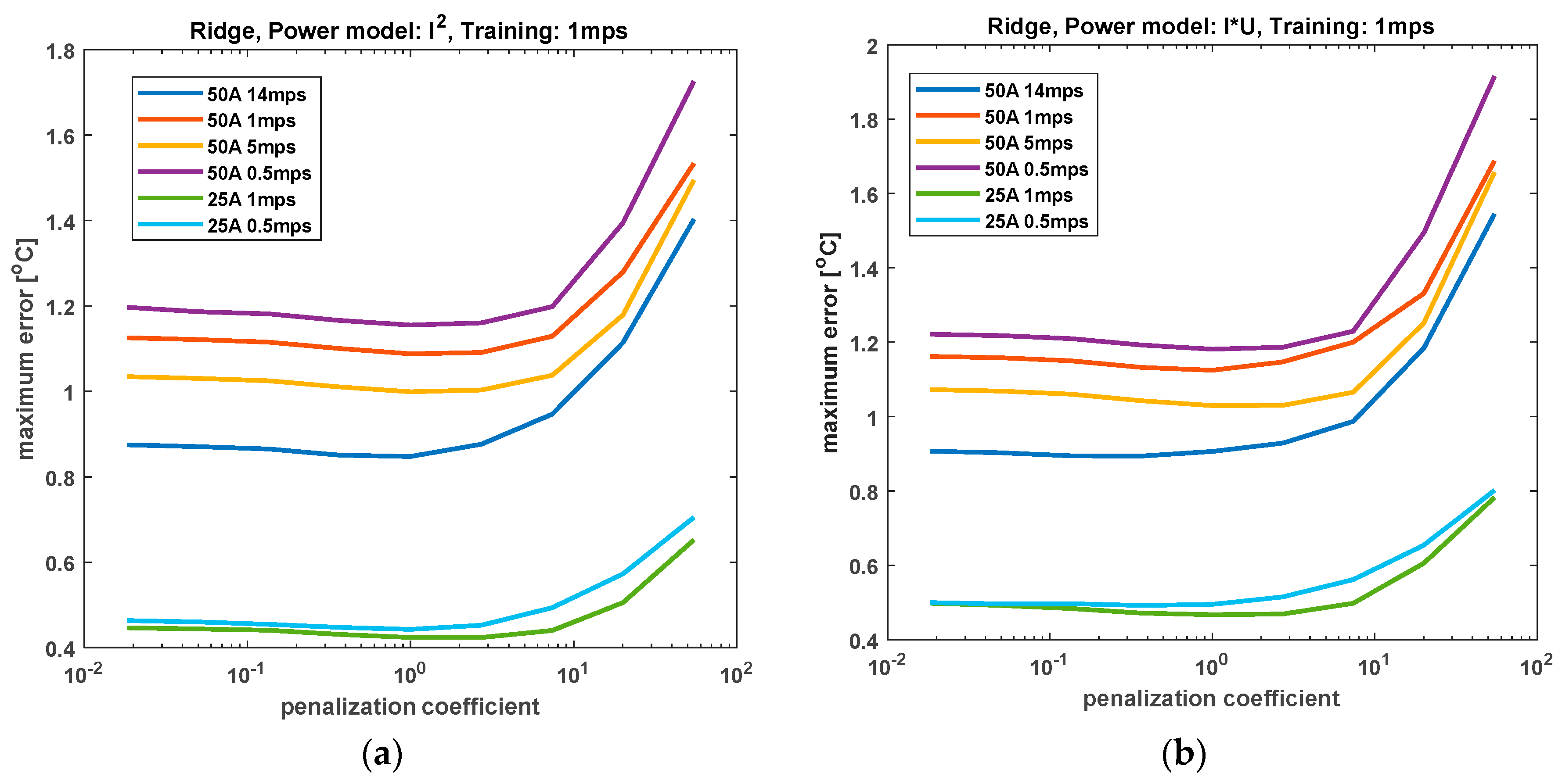
3.4. Tuning of Penalizations

While many methods for selection of the tuning coefficients are available, e.g., the L-curve method, we will use properties of our problem for its selection. Specifically, we aim to predict the temperatures $T$ in the regressor of model (1) using only predictions of previous values,

$$\begin{array}{rr}\hfill {\widehat{T}}_{m,k}& \hfill ={\displaystyle {\displaystyle \sum }_{i=1}^{\overline{i}}}\left({\displaystyle {\displaystyle \sum }_{l=1}^{\overline{l}}}\left(a_{m,l,i}{\widehat{T}}_{l,k-i}+z_{m,l,i}{P}_{l,k-i}\right)+c_{m,i}{T}_{\mathrm{bp},k-i}\right),\end{array}$$

(12)

Thus, prediction of the temperature profiles is a different task from fitting the known temperatures. Therefore, the risk of overfitting the model to the training data is minimized. Nevertheless, we will follow the conventional validation procedure and collect data from multiple experiments under different conditions. We will test if model parameters estimated from one experiments remain provide good performance on data from the remaining experiments.

4. TSEP Based Thermal Impedance Network Model

The performance of the new method proposed in the previous section has been compared with TSEP-based thermal impedance network model representing one of the best state-of-the-art methods.

4.1. Determination of Calibration Curve

TSEP methods for determining thermal impedances are based on the relationship between voltage and measured temperatures in the cool-down phase as shown in Figure 3. Though the temperature distribution is assumed to be homogenous in the cool-down phase, a discrepancy was observed in the temperatures measured from the heat sink sensor as well as those from the eight sensors placed closed to the transistors and diodes as shown in Figure 4a. Since the sensors were all of type Pt100, it is important to consider this discrepancy in the determination of the calibration curve. Hence, two calibration curves to establish the linear relationship between voltage and temperature are determined; one based on the maximum of the measured temperatures and the other based on the average values of the measured temperatures in the cool-down phase as shown in Figure 4b.

The thermal impedance network obtained using the maximum and average values of temperature yield slightly different results.

4.2. Thermal Impedance Network

The thermal impedance can be determined from the following Equation [22]:

$$Zth\left(t\right)=\frac{T_{Jnc}-T_H}{P}$$

(13)

T_H is the measured heatsink temperature, and P and T_Jnc are the transistor or diode power loss and junction temperatures, respectively.

For the VCE-based thermal impedances, the junction temperature is reconstructed from the relationship between the measured VCE and temperature obtained from the calibration curves in Figure 4b. Thermal impedances are also determined from the measured temperatures of the 8 Pt100 sensors.

By expressing the thermal impedance equation as shown in (13), curve-fitting techniques can be used in determining R_i and C_i (thermal impedances and capacitances, respectively).

$$Zth\left(t\right)={\displaystyle \sum }_{i=1}^n\left[R_i\times \left(1-e^{\frac{-t}{R_i\times C_i}}\right)\right]$$

(14)

Measurements at 50A and 5 m per second (m/s) air flowrate are used in determining the Zth parameters for different values of n (model order). The effect of the model order on the accuracy of the results is studied for both the thermal impedances obtained using VCE-based and measured temperatures from the Pt100 sensors. The Zth parameters obtained from 50A and 5 m/s flowrate are used in validating the model at different flowrates and currents.

5. Experimental Results

5.1. Experimental Results with Least Squares Method

From the set of experiments described in Section 2, we have used data recorded at 1 m/s flowrate and both steady-state currents (25 and 50A) as the training data. The remaining data sets are used for validation of accuracy of the method. We aim to validate accuracy of the method with growing order of the model and sensitivity of the results to the method evaluating the power input. However, as a first step, we need to determine the value of the regularization coefficient $\lambda$. We have estimated parameters of the tenth-order model on the training data sets (1 m/s 25A and 1 m/s 50A) and evaluated predictive temperatures (11) on all datasets. The maximum error of prediction (maximum is over time as well as all elements in the module) is displayed in Figure 5a for I² power model and Figure 5b for IU power model. In both cases, $\lambda =1$ seems to be a good choice.

With selected penalization of the regularization, we have tested sensitivity of the maximum prediction error to the order of the linear model (1). The results for the I² power model are displayed in Figure 6a and for the IU power model in Figure 6b. Note that the profile is almost the same for both power models. The prediction error is monotonically decreasing with the model order, reaching a plateau for orders higher than 5. This result is due to good selection of the regularization coefficient $\lambda$.

The 3rd order modelled top transistor temperature (model Equation (12)) and measured top transistor temperatures with $\lambda =1$ are shown in Figure 7.

5.2. Experimental Results with TSEP Method

Calibration curves for maximum and average measured temperatures are used in recomposing the junction temperatures for the transistors and diodes. As described in [22], the thermal impedances and capacitances are extracted by curve fitting methods from Equation (14). By placing the temperatures sensor closed to the transistors and diodes in the open IGBT module, the measured temperature is close to the junction temperature as observed by the infrared camera. Hence the measured temperatures are also used in establishing a thermal impedance network from which the junction temperature can be modelled.

Figure 8 shows maximum error against model (14) order for different currents and flowrates, for which the calibration curve for determining the thermal impedance network is obtained from the average of all measured temperatures in the cool-down phase as shown in Figure 4b. Figure 9 shows maximum error against model (14) order for different currents and flowrates for which the calibration curve for determining the thermal impedance network is obtained from the maximum of all measured temperatures in the cool-down phase as shown in Figure 4b. Figure 10 shows maximum error against model (14) order for different currents and flowrates for thermal impedance network determined from measured temperatures in the cool-down phase as shown in Figure 4b.

An important observation from Figure 8, Figure 9 and Figure 10 is that increasing the model order above 3 does not lead to significant improvements in the maximum and steady-state errors. This is important for implementation of a micro-controller for real-time calculation of junction temperature, where the processor throughput might be an issue.

The results obtained from all three thermal impedance networks (average VCE-based, maximum VCE-based and measured Pt100 temperature-based) for a 3rd order model (14) at a flowrate of 5 m/s are as shown in Figure 11. TTop is the measured top transistor temperature using the Pt100 sensor. TTopMax is the temperature estimated using the thermal impedance based on the calibration curve using a maximum of measured temperatures. TTopAvg is the temperature estimated using the thermal impedance based on the calibration curve using the average of measured temperatures. TTopMod is the temperature modelled from the thermal impedance determined from TTop. ErrMod is the difference between TTop and TTopMod, ErrMax is the difference between TTopMax and TTop, and ErrAvg is the difference between TTopAvg and TTop.

As shown in Figure 11, the maximum steady-state error is observed from the modelled temperature using the average value calibration curve. Maximum error is observed during the transition to the cooldown phase at the point when the transistor or diode is turned off. Steady-state errors between measured and model temperatures are within 1 °C, which confirms the accuracy of the models. In this paper, we focus not only on the maximum and steady-state errors from the modelling, but we also investigate the effect of model complexity (model order) against the maximum error. Since we define the thermal network as a multiple of 1^st-order systems connected in series, the model order in this case is defined as the number of first-order systems required by the thermal impedance network to accurately model the required junction temperature.

5.3. TSEP Method vs. Novel Least Squares Approach

Validation of modelled junction temperatures with directly measured temperatures with sensors placed close enough to active transistors or diodes is a common industrial practice. Manufacturers usually provide inverters with these capabilities in the product development phase. The proposed least-squares-based approach provides a better alternative approach to determining the junction temperature from such inverters. This approach eliminates the sources of error from the TSEP-based VCE methods, which rely heavily on the accuracy of the measured voltages across the transistors and diodes as well as those measured temperatures in the cooldown phase. Further sources of errors could result from the reconstruction of temperatures from the calibration curve, which are later used in the determination of the thermal impedance network.

Under the same operating conditions, the least squares method performs best with maximum temperature error of about 1.2 °C. On the other hand, the TSEP method based on the calibration curve determined from average measured temperatures in the cooldown has a maximum temperature error of 2 °C, while that of the TSEP method based on calibration curve determined from the maximum measured temperatures in the cool-down phase has a maximum temperature error of 3.5 °C.

6. Conclusions

We compared the quality of prediction of the temperature of all elements in a power module using direct temperature measurements. We have shown that coefficients of the linear transfer function from the power input to the temperature can be estimated by the least squares methods with ridge regression. For a well-chosen penalization, the proposed method provided more accurate results than the industry-standard TSEP method. We have tested two models of the power input, one based on measurement of voltage drop and the second based on estimating coefficients of the second-order approximation of the power from the current. Both power models achieved comparable accuracy. The proposed method is accurate and simple to use when direct temperature measurements are available.

References

1. Blackburn, D. Temperature measurements of semiconductor devices—A review. In Proceedings of the Twentieth Annual IEEE Semiconductor Thermal Measurement and Management Symposium, San Jose, CA, USA, 11 March 2004. [Google Scholar]
2. Niu, H.; Lorenz, R.D. Sensing IGBT junction temperature using gate drive output transient properties. In Proceedings of the IEEE Applied Power Electronics Conference and Exposition (APEC), Charlotte, NC, USA, 15–19 March 2015. [Google Scholar]
3. Achiri, H.M.N.; Smidl, V.; Peroutka, Z. Mitigation of electric drivetrain oscillation resulting from abrupt current derating at low coolant flow rate. In Proceedings of the 41st Annual Conference of the IEEE Industrial Electronics Society, Yokohama, Japan, 9–12 November 2015. [Google Scholar]
4. Huang, H.; Mawby, P.A. A Lifetime Estimation Technique for Voltage Source Inverters. IEEE Trans. Power Electron. 2013, 28, 4113–4119. [Google Scholar] [CrossRef]
5. Choi, U.-M.; Blaabjerg, F.; Jørgensen, S. Study on Effect of Junction Temperature Swing Duration on Lifetime of Transfer Molded Power IGBT Modules. IEEE Trans. Power Electron. 2017, 32, 6434–6443. [Google Scholar] [CrossRef] [Green Version]
6. Tran, S.H.; Khatir, Z.; Lallemand, R.; Ibrahim, A.; Ousten, J.P.; Ewanchuk, J.; Mollov, S.V. Constant ΔTj Power Cycling Strategy in DC Mode for Top-Metal and Bond-Wire Contacts Degradation Investigations. IEEE Trans. Power Electron. 2019, 34, 2171–2180. [Google Scholar] [CrossRef]
7. Chen, H.; Ji, B.; Pickert, V.; Cao, W. Real-Time Temperature Estimation for Power MOSFETs Considering Thermal Aging Effects. IEEE Trans. Device Mater. Reliab. 2013, 14, 220–228. [Google Scholar] [CrossRef]
8. Asimakopoulos, P.; Papastergiou, K.; Thiringer, T.; Godec, G.L. On Vce Method: In Situ Temperature Estimation and Aging Detection of High-Current IGBT Modules Used in Magnet Power Supplies for Particle Accelerators. IEEE Trans. Ind. Electron. 2018, 66, 551–560. [Google Scholar] [CrossRef]
9. Vogel, K.; Ciliox, A.; Schmal, A. IGBT with higher operation temperature-Power density, lifetime and impact on inverter design. In Proceedings of the PCIM Europe, Nuremberg, Germany, 17–19 May 2011. [Google Scholar]
10. Plesca, A. Thermal Analysis of Power Semiconductor Device in Steady-State Conditions. Energies 2019, 13, 103. [Google Scholar] [CrossRef] [Green Version]
11. Musallam, M.; Buttay, C.; Whitehead, M.; Johnson, M. Real-time compact electronic thermal modelling for health monitoring. In Proceedings of the European Conference on Power Electronics and Applications, Aalborg, Denmark, 2–5 September 2007. [Google Scholar]
12. Murdock, D.; Torres, J.; Connors, J.; Lorenz, R. Active thermal control of power electronic modules. IEEE Trans. Ind. Appl. 2006, 42, 552–558. [Google Scholar] [CrossRef] [Green Version]
13. Musallam, M.; Acarnley, P.; Johnson, C.; Pritchard, L.; Pickert, V. Estimation and control of power electronic device temperature during operation with variable conducting current. IET Circuits Devices Syst. 2007, 1, 111–116. [Google Scholar] [CrossRef]
14. Yu, Y.; Lee, T.-Y.T.; Chiriac, V.A. Compact Thermal Resistor-Capacitor-Network Approach to Predicting Transient Junction Temperatures of a Power Amplifier Module. IEEE Trans. Compon. Packag. Manuf. Technol. 2012, 2, 1172–1181. [Google Scholar] [CrossRef]
15. Gorecki, K.; Zarebski, J. Nonlinear Compact Thermal Model of Power Semiconductor Devices. IEEE Trans. Compon. Packag. Technol. 2010, 33, 643–647. [Google Scholar] [CrossRef]
16. Sofia, J. Analysis of thermal transient data with synthesized dynamic models for semiconductor devices. IEEE Trans. Compon. Packag. Manuf. Technol. 1995, 18, 39–47. [Google Scholar] [CrossRef]
17. Rencz, M.; Szekely, V. Dynamic thermal multiport modeling of IC packages. IEEE Trans. Compon. Packag. Technol. 2001, 24, 596–604. [Google Scholar] [CrossRef]
18. Wu, R.; Wang, H.; Ma, K.; Ghimire, P.; Iannuzzo, F.; Blaabjerg, F. A temperature-dependent thermal model of IGBT modules suitable for circuit-level simulations. In Proceedings of the 2014 IEEE Energy Conversion Congress and Exposition, Pittsburgh, PA, USA, 14–18 September 2014. [Google Scholar]
19. Filicori, F.; Bianco, C.G.L. A simplified thermal analysis approach for power transistor rating in PWM-controlled DC/AC converters. IEEE Trans. Circuits Syst. I Fundam. Theory Appl. 1998, 45, 557–566. [Google Scholar] [CrossRef] [Green Version]
20. Yun, C.-S.; Malberti, P.; Ciappa, M.; Fichtner, W. Thermal component model for electrothermal analysis of IGBT module systems. IEEE Trans. Adv. Packag. 2001, 24, 401–406. [Google Scholar]
21. Luo, Z.; Ahn, H.; Nokali, M.A.E. A thermal model for insulated gate bipolar transistor module. IEEE Trans. Power Electron. 2004, 19, 902–907. [Google Scholar] [CrossRef]
22. Achiri, H.M.N.; Streit, L.; Smidl, V.; Peroutka, Z. Experimental validation of IGBT thermal impedances from voltage-based and direct temperature measurements. In Proceedings of the Annual Conference of the IEEE Industrial Electronics Society, Florence, Italy, 23–26 October 2016. [Google Scholar]
23. Whitehead, M.J.; Johnson, C.M. Junction Temperature Elevation as a Result of Thermal Cross Coupling in a Multi-Device Power Electronic Module. In Proceedings of the 1st Electronics Systemintegration Technology Conference, Dresden, Germany, 5–7 September 2006. [Google Scholar]
24. Avenas, Y.; Dupont, L.; Khatir, Z. Temperature Measurement of Power Semiconductor Devices by Thermo-Sensitive Electrical Parameters—A Review. IEEE Trans. Power Electron. 2011, 27, 3081–3092. [Google Scholar] [CrossRef] [Green Version]
25. Dupont, L.; Avenas, Y.; Jeannin, P.-O. Comparison of Junction Temperature Evaluations in a Power IGBT Module Using an IR Camera and Three Thermosensitive Electrical Parameters. IEEE Trans. Ind. Appl. 2013, 49, 1599–1608. [Google Scholar] [CrossRef] [Green Version]
26. Khatir, Z.; Carubelli, S.; Lecoq, F. Devices, Real-time computation of thermal constraints in multichip power electronic. IEEE Trans. Compon. Packag. Technol. 2004, 27, 337–344. [Google Scholar] [CrossRef]
27. Chibante, R.; AraÚjo, A.; Carvalho, A. Finite-Element Modeling and Optimization-Based Parameter Extraction Algorithm for NPT-IGBTs. IEEE Trans. Power Electron. 2009, 24, 1417–1427. [Google Scholar] [CrossRef]
28. Dornic, N.; Khatir, Z.; Tran, S.H.; Ibrahim, A.; Lallemand, R.; Ousten, J.-P.; Ewanchuk, J.; Mollov, S.V. Stress-Based Model for Lifetime Estimation of Bond Wire Contacts Using Power Cycling Tests and Finite-Element Modeling. IEEE J. Emerg. Sel. Top. Power Electron. 2019, 7, 1659–1667. [Google Scholar] [CrossRef]
29. Raciti, A.; Cristaldi, D. Thermal modeling of integrated power electronic modules by a lumped-parameter circuit approach. In Proceedings of the AEIT Annual Conference, Mondello, Italy, 3–5 October 2013. [Google Scholar]
30. Fabio, D.N.; Alessandro, M.; Marino, C.; Pierluigi, G.; Vincenzo, D.; Lorenzo, C.; Pietro, T.; Santolo, D. On-Line Junction Temperature Monitoring of Switching Devices with Dynamic Compact Thermal Models Extracted with Model Order Reduction. Energies 2017, 10, 189. [Google Scholar]
31. Wang, Z.; Qiao, W. An Online Frequency-Domain Junction Temperature Estimation Method for IGBT Modules. IEEE Trans. Power Electron. 2015, 30, 4633–4637. [Google Scholar] [CrossRef]
32. Gachovska, T.K.; Tian, B.; Hudgins, J.L.; Qiao, W.; Donlon, J.F. A Real-Time Thermal Model for Monitoring of Power Semiconductor Devices. IEEE Trans. Ind. Appl. 2015, 51, 3361–3367. [Google Scholar] [CrossRef]
33. Eleffendi, M.A.; Johnson, C.M. Application of Kalman Filter to Estimate Junction Temperature in IGBT Power Modules. IEEE Trans. Power Electron. 2015, 31, 1576–1587. [Google Scholar] [CrossRef]
34. Hoerl, E.; Kennard, R.W. Ridge regression: Biased estimation for nonorthogonal problems. Technometrics 1970, 12, 55–67. [Google Scholar] [CrossRef]
35. Tipping, M.E. Sparse Bayesian Learning and the Relevance Vector Machine. J. Mach. Learn. Res. 2001, 1, 211–244. [Google Scholar]
Figure 1. Direct temperature measurement test bench. (a) infrared camera; (b) Eight temperature sensors; (c) open IGBT module; (d) cooling fan.
Energies 13 03749 g001
Figure 2. Circuit used in direct and thermo-sensitive electrical parameter (TSEP)-based temperature measurement.
Energies 13 03749 g002
Figure 3. Temperature, current, and voltage profiles during measurement.
Energies 13 03749 g003
Figure 4. (a) Measured temperatures in cool-down phase; (b) Calibration curves determined from maximum and average of measured temperatures.
Energies 13 03749 g004
Figure 5. Maximum error vs. penalization coefficient ridge regression (a) I2 power model (b) IU power model.
Energies 13 03749 g005
Figure 6. Maximum error vs. model order least squares (a) I2 power model (b) IU power model.
Energies 13 03749 g006
Figure 7. Measured vs. least-squares model temperature 3rd order top transistor active 50A 5 m/s air flowrate.
Energies 13 03749 g007
Figure 8. Maximum error vs. model order for collector–emitter voltage (VCE) method with calibration curve from average temperature in cooldown phase.
Energies 13 03749 g008
Figure 9. Maximum error vs. model order for VCE method with calibration curve from maximum temperature in cooldown phase.
Energies 13 03749 g009
Figure 10. Maximum error vs. model order for measured Pt100 temperatures.
Energies 13 03749 g010
Figure 11. Measured vs. model temperatures 3rd order top transistor active 50A 5 m/s air flowrate.
Energies 13 03749 g011