Proving a Concept of Flexible Under-Frequency Load Shedding with Hardware-in-the-Loop Testing

Abstract

It is widely recognized that in the transition from conventional electrical power systems (EPSs) towards smart grids, electrical voltage frequency will be greatly affected. This is why this research is extremely valuable, especially since rate-of-change-of-frequency (RoCoF) is often considered as a potential means of resolving newly arisen problems, but is often challenged in practice due to the noise and its oscillating character. In this paper, the authors further developed and tested one of the new technologies related to under-frequency load shedding (UFLS) protection. Since the basic idea was to enhance the selected technology’s readiness level, a hardware-in-the-loop (HIL) setup with an RTDS was assembled. The under-frequency technology was implemented in an intelligent electronic device (IED) and included in the HIL setup. The IED acted as one of several protection devices, representing a last-resort system protection scheme. All main contributions of this research deal with using RoCoF in an innovative UFLS scheme under test: (i) appropriate selection and parameterization of RoCoF filtering techniques does not worsen under-frequency load shedding during fast-occurring events, (ii) locally measured RoCoF can be effectively used for bringing a high level of flexibility to a system-wide scheme, and (iii) diversity of relays and RoCoF-measuring techniques is an advantage, not a drawback.

1. Introduction

In most of the developed world, EPSs are known for their robustness, efficiency and extremely high reliability. It comes as no surprise that throughout the decades, this reputation eventually resulted in most of the population taking the electrical energy supply for granted. If it were not for the significant environmental impact of associated activities, such as electrical energy generation and its transmission, no noteworthy changes would be imposed on EPSs in the near future. However, the reality of climate-related concerns has driven the need for technological development to such a level that the conventional electrical energy supply paradigm was placed in front of a challenge none of us had ever faced before. Among others, the sector of electrical energy generation is the most notable example. In a relatively short period of time, significant portions of conventional centralized generating capacities were replaced by distributed renewable energy sources, mostly interfacing with EPSs via semi-conductive power converters [1]. This can be seen as both a blessing and a curse, since power converters are indeed able to provide a convenient fast-acting intervention, but unfortunately not inherently.

The transition towards converter-based generation caused the vast amount of energy temporarily stored within rotating masses of conventional power plants in the form of rotational kinetic energy to decrease quickly [2]. This energy serves as a buffer when sudden active power imbalances occur in the EPS, providing a limited energy source for a temporary load supply [3]. Withdrawing the rotating energy causes generators to decelerate. The deceleration rate depends on the amount of power imbalance and the overall stored rotational kinetic energy. As a consequence, conventional EPSs are not prone to significant RoCoF. Consequently, the more we advance toward the smart grid paradigm, the more frequency (among several others quantities), measured from electrical signals (voltage, current), becomes affected [4,5].

For decades, frequency stability was of no concern to transmission system operators (TSOs). An evident proof of this is the applied UFLS schemes in most developed networks around the world. Apart from a few exceptions in countries whose isolated EPS of smaller dimensions is asynchronously connected to larger interconnections, the great majority of them still use an approach introduced decades ago (known as the conventional or traditional UFLS concept). The research community recognized the problem of neglecting UFLS development quite some time ago, which resulted in an impressive number of scientific publications (e.g., the latest [6,7,8,9,10,11]). Yet, most of those published methods appear complex and require the use of advanced mathematical techniques, several of which are non-transparent. Many of the methods rely either on real-time communication between a vast number of protective devices all across the EPS [12,13] or the assumption of having accurate enough information about the involved EPS inertia [14,15,16]. As a result, apart from a few individual pilot projects, no significant progress has been made in this field so far, especially concerning practical applicability.

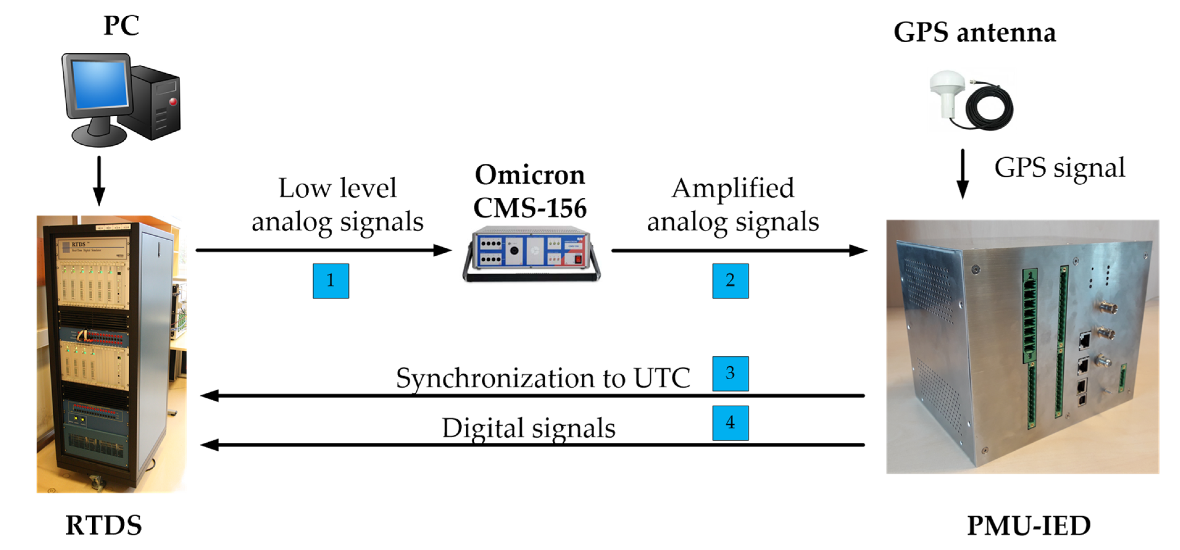
In this paper, we present a procedure for proving the concept of an innovative and practically feasible UFLS [17] in terms of HIL simulations. For this purpose, a real-time digital simulator (RTDS) was applied together with an IED selected for running a local UFLS algorithm. IED is a commonly used term in the electric power industry to describe microprocessor-based controllers of EPS equipment [18]. During the HIL testing of the innovative UFLS method, we have developed a few improvements related to a more straightforward deployment of the method: (i) improved filtering for better resolution and filtering of anomalies, (ii) a proof that despite the RoCoF filtering, introduced time delays do not diminish the speed of UFLS, and (iii) easy deployment of the method on the existing IED-based devices. For the reader’s convenience, a brief summary of the new UFLS methodology from [17] is provided in Section 2, together with the IED-related implementation challenges and provided solutions for the applicability of the method in a real environment. This is followed by the specifics of the experimental HIL setup in Section 3 and the simulation results in Section 4. Finally, the conclusions are drawn in Section 5.

2. Methods

2.1. Innovative Use of Rate-of-Change-of-Frequency

The UFLS method, summarized in this section, was previously published in [17] and evaluated in an off-line EPS-dynamics simulation tool PSS Netomac, which is a part of the PSS SINCAL Platform [19]. From this point on, it will be referred to as innovative UFLS. Since it is of great importance for the reader to be acquainted with its main philosophy, it seems reasonable to provide its brief explanation in this paper as well. After all, this paper is specifically about proving that the concept works in an environment as close as possible to real-life conditions and providing the required improvements for final deployment.

The first cornerstone of the innovative UFLS method [17] is the on-line calculation of the frequency stability margin M(t) at all frequency relay locations across the EPS. M(t) is a time-dependent variable that is, in its essence, the worst-case estimated time before the EPS frequency f(t) is expected to violate the predefined frequency stability limit (f_LIM). For this purpose, an assumption is made that if none of the frequency control/protection functionalities intervene, the f(t) variation will follow the same trend as indicated by the respective RoCoF(t) measurement at the same instant. The local nature of the EPS frequency dynamics that follows an active power imbalance ΔP incident means that in a selected point in time, the calculated M(t) is different in every busbar in the system (due to the oscillating nature of the EPS [20]). In Figure 1a, the blue and yellow curves depict the EPS frequency response to two unequal ΔP incidents (ΔP₁ and ΔP₂ respectively) assumed to have taken place in the same busbar. At moment t = t₁, respective RoCoF(t₁) indicates different M(t₁) values, depending on the underlying ΔP incident. It is clear from Figure 1a that ΔP₁ caused a less serious frequency excursion compared to ΔP₂. This manifests in a larger M(t₁) value, an indicator of having more time before f_LIM is reached.

The second cornerstone of [17] is an innovative representation of conditions in the f(t) versus M(t) diagram (Figure 1b). After the ΔP incident, the operating point in the f(t)-M(t) diagram begins to drift along the corresponding trajectory that points towards one of two possible directions: (i) coordinates (M = 0, f = f_LIM) in the lower left part of the diagram (blue curve) or (ii) far away from the ordinate axis in the right-hand side of the diagram (yellow curve). This conclusion makes one able to define a new, double-criteria UFLS tripping function for each UFLS stage. The first criterion remains identical to conventional UFLS, being the violation of a predefined frequency threshold f_thr. The second criterion, on the other hand, is a violation of a predefined stability threshold M_thr and is monitored independently of the first. Only when both tripping criteria are simultaneously fulfilled, the trip signal is generated. A simplified logical diagram of the process is presented in Figure 2 since the detailed version is a subject to an international patent application submitted by the University of Ljubljana.

For the reader’s convenience, it appears reasonable at this point to describe the simplified logical diagram of the innovative UFLS process in Figure 2. Since the main task of UFLS is to handle frequency-decaying situations, the input RoCoF(t) value is limited to only negative values (indicating a frequency drop). Next, the calculation of a frequency stability margin M(t) requires the division with a RoCoF(t) value, which is a consequence of applying a simple linear relationship graphically described in Figure 1a. Since in stable cases the RoCoF(t) value is constantly somewhere around zero, it is reasonable to provide an upper limit of RoCoF(t) to a value slightly below zero. Our analysis showed that this simple precaution successfully stabilizes the division process. In the continuation, the frequency and frequency stability thresholds are checked independently for a potential violation and the trip signal is generated only when both criteria are met simultaneously (logic AND gate).

The most important feature of the described UFLS concept is that any RoCoF-related variety (be it the diverse local frequency dynamics in the network or the diverse relay equipment performing RoCoF calculation procedures and filtering techniques) is inherently converted into an important advantage. The resulting variety of calculated M(t) values across the network causes the M_thr criterion not being violated simultaneously in different locations. This can be seen as if one is dealing with a much larger number of UFLS stages, which can eventually manifest as a fine-tuning of UFLS (further explained in the continuation of this paper).

2.2. Intelligent Electronic Device

For the purpose of RTDS testing of the innovative UFLS methodology presented in Section 2.1, we used an IED based on our in-house developed and fully functional phasor measurement unit (PMU). Therefore, to avoid any misunderstandings, from this point onward this device will be referred to as PMU-IED. In the first step, the PMU-IED was tested for whether its primary function was suitable for use in the innovative UFLS. For evaluation purposes, we used one of the commercially available PMUs, referred to as PMU-COMM. Both PMUs are compliant with the latest revision of IEEE Std C37.118.1-2011 [21]. The advantages of deriving an IED from a PMU are mainly the compelling features that the PMU-IED offers, such as the 200 Hz reporting rate (F_S), high accuracy and short response times, input/output (I/O) ports and real-time processing. By modifying the external quantities according to the needs of the innovative UFLS method, we obtained a fully functional IED device that is ready for deployment.

In the first set of tests, we have extensively tested the response of both the PMU-IED and the PMU-COMM along with an internal software-based PMU (since the RSCAD software we are referring to is a part of the RTDS simulator, the internal PMU-8 model is denoted as PMU-RTDS). For the PMU-IED and PMU-COMM, we used maximal reporting rates of 200 Hz and 50 Hz respectively. For benchmarking purposes, the PMU-RTDS was set to have a 200 Hz reporting rate. The first thing that was noticed was that the PMU-RTDS represents an ideal case where any kind of environmental noise does not influence the measured quantities, which is not the case for the PMU-IED and PMU-COMM devices. To support this claim, a simulation of a significant amount of active power deficit, which causes the RoCoF to suddenly change from the value of zero to approximately −0.4 Hz/s, is presented in Figure 3a. As expected, the PMU-RTDS generates the RoCoF result almost completely without noise (red curve in Figure 3a), since the only limiting feature is the finite precision of representing floating-point numbers and the implemented frequency estimation method in the hardware. On the other hand, both physical devices under test, the PMU-IED (cyan curve) and the PMU-COMM (black curve), show a high degree of fluctuation/noise around expected values. This is because, in its essence, RoCoF is the derivate of frequency. As a result, any small and fast variations of frequency are most likely to be amplified in RoCoF [22]. As expected, these fluctuations have a high impact on the innovative UFLS (see Figure 3b). Therefore, RoCoF filtering needed to be addressed first.

2.3. Rate-of-Change-of-Frequency Filtering

By definition, RoCoF is a time derivate of the frequency f:

$$RoCoF=\frac{df}{dt}\approx \frac{\mathsf{\Delta }f}{\mathsf{\Delta }t}=\mathsf{\Delta }f·F_S$$

(1)

Thus, high fluctuations are expected in RoCoF in a noisy environment when one is dealing with a high reporting rate F_S. To decrease the noise, we could lower F_S, but this would lead to a slower response of the UFLS system depending on RoCoF. This is why it is of utmost importance to find the optimal response of the UFLS system while still getting meaningful values for RoCoF. In Figure 4, the 200-ms-long windowing function was added to the RoCoF calculation (to both the PMU-IED and the PMU-COMM) that averages all samples (moving average) in the window. Averaging reduces the system response capabilities since, with a longer window, it passes only the DC component in its limit in the frequency domain. As seen in Figure 4, the moving average filter greatly improves the RoCoF reported by both devices. On the other hand, this is achieved on account of having a higher output delay (around half of the window length, i.e., ≈100 ms, which can be noticed as a shift of the PMU-IED and PMU-COMM curves with respect to the PMU-RTDS), which is also reflected in the f(t)-M(t) diagram (Figure 4b).

As expected, the PMU-COMM shows lesser improvement compared to the PMU-IED since it has a lower F_S (50 Hz) and the noise reduction is related to the square root of points used in the window [23].

In the next phase, we put our focus on the RoCoF report dynamics after a discrete active power balancing event occurs in the EPS (either initial event causing frequency to deviate from the nominal value or a UFLS intervention). In this case, the simulated power imbalance incident was twice as large, so the RoCoF reaches values up to −0.80 Hz/s. Such events taking place result in momentarily distorted measured electrical quantities (voltages, currents) and, consequently, both the frequency and RoCoF as well. For the sake of clarity, a set of raw measurements (without the moving average filtering described above) are presented in Figure 5 for the case where the conventional UFLS scheme operates at thresholds of 49.0, 48.8, and 48.6 Hz after the EPS was subject to a power imbalance incident.

After each event related to power balance, numerical oscillations are present in both the frequency and RoCoF reports (Figure 5a), which is manifested in the f(t)-M(t) diagram (Figure 5b) as a significant deviation from the expected trajectory. These momentary oscillations needed to be filtered out in frequency and especially in RoCoF. The performed analysis showed that after every event, the RoCoF momentarily increased in amplitude for several orders. Thus, one of the non-linear filtering techniques is required; otherwise (by using a moving average or similar linear-based filter), the unwanted oscillation will disperse along the time axis, resulting in the need for a long linear-based filter that would generate undesirable delays. Eventually, the use of such RoCoF in innovative UFLS might cause unexpected load tripping (shedding) and fail the power re-balancing.

After careful consideration, we implemented the median filter whose impact on RoCoF reports along with the moving average filtering is depicted in Figure 6. Figure 6b shows that the described approach is successful in filtering out all disruptive anomalies and noise without scarifying the response time. Finally, the PMU-IED was modified accordingly by changing the default output filter (the one that complies with the IEEE C37.118 standard [24,25]) with a combination of filters as shown in Figure 7. A thorough investigation revealed that the depicted sequence of filtering represents an optimal combination. First, the moving average filter (window length of 40 ms) improves the RoCoF resolution and decreases the noise. Next, the median filter (window length of 110 ms), which proved itself to be much more efficient with an existing 40 ms pre-filtering by the moving average filter, handles the numerical anomalies. Finally, the second part of the moving average filtering (window length of 100 ms) can further improve the resolution of the measurement for the sake of time delay.

As far as the frequency is concerned, a median filter (window length of 110 ms) was adequate to solve the issue without causing any unwanted UFLS behavior.

3. Experimental Setup

3.1. HIL Setup—Overview

The assembled HIL setup consists of five hardware elements: (i) an RTDS simulator, (ii) an Omicron CMS-156 amplifier, (iii) a PMU-IED, (iv) a global-positioning system (GPS) antenna, and (v) a personal computer (PC) which runs the RSCAD software and represents a human-machine interface for accessing the simulated part of the setup. An overview of a HIL arrangement is shown in Figure 8.

3.1.1. Real-Time Digital Simulator

The RTDS simulates the operation of EPSs using parallel processing architecture that is specifically designed to solve the transient electromagnetic simulation (EMT) algorithm in real-time. The RSCAD interface software allows the user to perform all the necessary steps to prepare and run simulations as well as visualize the results. Apart from processor cards, which present the main driving core of the simulator itself, the RTDS contains analogue and digital input/output channels that enable communication with external physical devices. This is achieved by means of a specialized analogue output card that is used to produce analogue waveforms (see blue-shaded annotation 1 in Figure 8) expected by the PMU-IED terminals. However, it is worth noting that the GTAO card produces a low-level analogue signal with a maximum of ±10 V peak. Even though some IEDs can accept such low-level signals directly (including the PMU-IED), this is not generally the case. To create a more generalized testing platform, low-level signals were scaled up with an amplifier (see blue-shaded annotation 2 in Figure 8) before being fed to the PMU-IED. In contrast, for the purposes of the UFLS scheme, the shedding signal generated by the PMU-IED is in a digital format (see blue-shaded annotation 4 in Figure 8). A specialized digital input card in the RTDS simulator was therefore used to bring the shedding/trip command back into the simulation and close the testing loop.

Another very important aspect of HIL testing is to keep all participating devices in synchronism. A so-called GTSYNC card ensures that the simulator time-step remains locked to the GPS signal, using either the IEEE 1588 precision time protocol (PTP), 1 pulse per second (PPS) or an inter-range instrumentation group time code format B (IRIG-B) signal. The proposed test setup used the PPS signal provided by the PMU-IED as the synchronization source (see blue-shaded annotation 3 in Figure 8).

3.1.2. Omicron CMS-156 Amplifier

The omicron CMS-156 amplifier features a three-phase voltage with neutral outputs and a three-phase current with neutral outputs that are galvanically isolated from the inputs. The amplifier can produce three current signals of up to 25 A each and three voltage signals of up to 250 V each. At a nominal frequency of 50/60 Hz, the amplifier introduces 1.88°/2.26° of phase lag for current outputs and 1.95°/2.34° of phase lag for voltage outputs respectively. For the purposes of HIL testing, phase lags need to be properly accounted for. In the proposed HIL setup, the calibration offset angles of the PMU-IED were set accordingly.

3.2. HIL Setup—Intelligent Electronic Device

A physical PMU-IED, described in Section 2.2, requires a three-phase voltage input that is used for calculating the frequency f(t) and RoCoF(t). The voltages that have to be appropriately amplified (see Section 3.1) are supplied to the PMU-IED by the RTDS simulator. On the output side, the PMU-IED device enables six digital outputs (logical type 0/1) used as trip signals for each of the six UFLS stages (see

Table 1. Conventional UFLS setting (frequency thresholds f_thr) along with supplemented frequency stability margin (M_thr) thresholds.

UFLS Stage Number	${\mathit{f}}_{\mathbf{t}\mathbf{h}\mathbf{r}}\left[\mathbf{Hz}\right]$	${\mathit{M}}_{\mathbf{t}\mathbf{h}\mathbf{r}}\left[\mathbf{s}\right]$	EPS Load Decrease [%]
1.	49.0	6.0	10
2.	48.8	5.0	10
3.	48.6	4.0	10
4.	48.4	3.0	10
5.	48.2	2.0	10
6.	48.1	1.0	5

). These signals control the circuit-breaker models within the RTDS, influencing the connection status of an individual EPS load.

However, our laboratory capacities enabled us to include only one physical PMU-IED device in the HIL experiments. In order for the overall UFLS scheme to function correctly, we had to build a RTDS computer model of all PMU-IED devices that were not physically present in the laboratory. For this purpose, a computer model of innovative UFLS was created in C-builder, running on f(t) and RoCoF(t) measurements provided by the PMU-RTDS internally within the RTDS.

The RTDS simulator used in this paper can be handled through an RSCAD software environment [26]. Apart from modelling elementary EPS elements (main high-voltage components, protection and control functions), RSCAD enables the user to create custom-built components in a module C-builder. Once created, any user-defined component is used in the same manner as any other component from the RSCAD library.

To create a representative copy of the PMU-IED in the RTDS simulator, the same amount of UFLS stages had to be allowed in the model as well. To make it more general, we decided to allow the user to specify an arbitrary number of UFLS stages (up to six). A corresponding number of outputs is also enabled. Apart from that, a f_LIM and all threshold values (f_thr and M_thr) can be provided separately, together with window widths for filtering described in Figure 7.

To verify the computer model of the PMU-IED running innovative UFLS logic, we performed a large number of tests. Eventually, we were able to prove a satisfying compliance of the physical and the modelled PMU-IED.

3.3. HIL Setup—Electric Power System

We adopted an IEEE 9-bus benchmark EPS as a basis, whose parameters and other specifics can be found in [3]. This benchmark model consists of three synchronous generators (denoted by G1, G2 and G3 in Figure 9) together with corresponding step-up transformers, six transmission lines and three equivalent loads (denoted by L5, L6 and L8). All machines are controlled by their respective governor and excitation controllers. The total installed generating power is 567.5 MVA and 10% of each machine’s rated power is selected to attribute to frequency control purposes, whereas loads are modelled as a constant impedance.

To use this benchmark model for UFLS testing, several modifications had to be applied (Figure 9). First, each of the three equivalent loads (L5, L6 and L8) was split into seven partitions. Six of them correspond to individual UFLS stages (see Table 1) denoted by L_x-UFLS where subscript “x” represents the number of the corresponding busbar. The seventh partition, however, represents the remaining aggregation of all the consumers not included in the UFLS scheme (L_x-S). Second, an infinite power source was additionally introduced to the model, busbar 4, to be more specific. Its disconnection was considered the main event causing active power deficit conditions in the newly formed island. With this, many different power conditions can be simulated by changing the steady-state production of all three generating units prior to the main event. An infinite power source in all cases supplies/consumes enough power to meet the power balance in a steady-state. Once disconnected, an EPS island is formed with a certain imbalance between the production and the consumption of active and reactive powers. In this paper, circumstances with a lack of active power were simulated, which cause an EPS frequency to decay and consequently trigger UFLS.

Lastly, devices performing UFLS were included in the model. A single physical PMU-IED was fed by voltage U₅ on busbar 5 and was able to disconnect loads L₅-UFLS according to Table 1. The other two load busbars (6 and 8) were monitored and controlled with a PMU-RTDS component within a simulated environment, fed by voltages U₆ and U₈, respectively.

4. Results

Both the conventional six-stage UFLS scheme currently used in Slovenia and the innovative UFLS scheme were applied in simulation scenarios. Specifics of both UFLS settings are provided in Table 1. Frequency thresholds f_thr are taken from the Slovenian Grid code [27], and additional frequency stability margin thresholds M_thr are selected with a one-second span between them since the analysis showed there are no special differences when selected otherwise.

In the base case, steady-state conditions before the main event were set so that the total loading of the benchmark IEEE 9-bus system model (Figure 9) was 315 MW and the overall generating power was 319.6 MW. Apart from the base case, this research included 65 additional simulated cases (66 altogether), in which the total generation capacity before the main event was gradually decreased by 1% per case. In this way, the amount of power provided by the power source (and consequently power mismatch between the generation and the consumption) in the moment of a simulated switching event increased with each consecutive case. This was repeated to the point where all available frequency control and protection mechanisms (primary frequency control and UFLS) were insufficient to prevent frequency decay bellow the f_LIM.

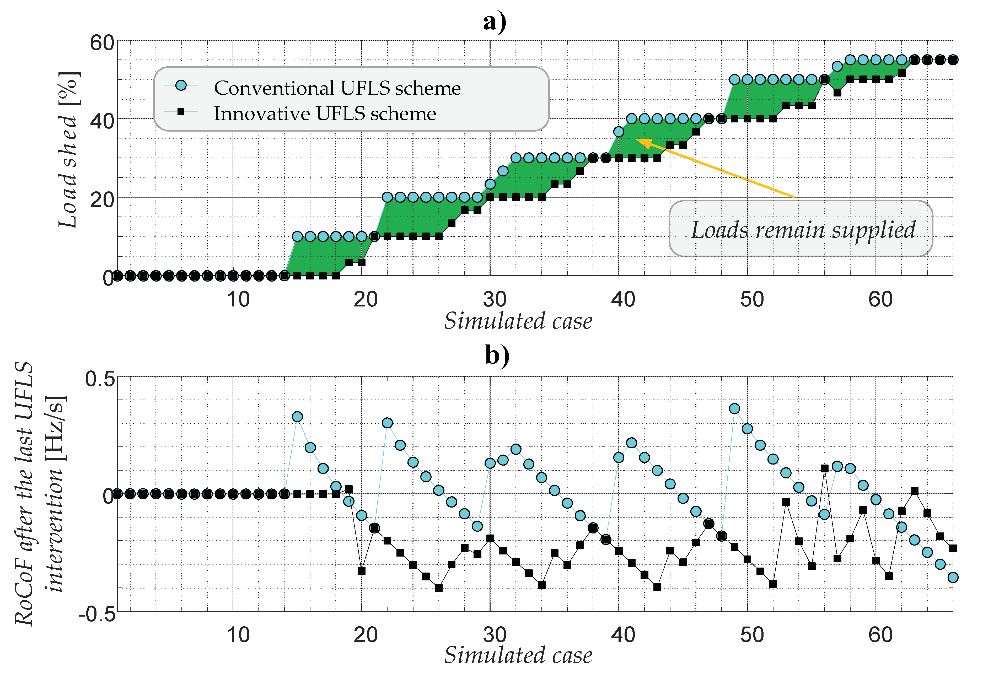
In Figure 10, an overview of the results extracted from the entire set of 66 simulated cases is provided. Cases are listed on the horizontal axis. Conventional UFLS results are depicted with cyan markers, whereas black markers correspond to innovative UFLS. Figure 10a shows the percentage of the EPS de-loading due to UFLS. Conventional UFLS is activated in 79% of all cases (52 out of 66). Among these, innovative UFLS keeps more load supplied in 81% of cases (42 out of 52) while still being successful in achieving frequency stabilization. This is marked by a green-shaded area between the two curves in Figure 10a.

Another thing worth mentioning is that with a conventional UFLS scheme, shedding in all three busses will nearly always take place simultaneously (92% of cases/48 out of 52 cases) and, consequently, the entire UFLS stage will be tripped. However, partial UFLS activation is much more frequent for the innovative UFLS scheme (31% of cases/16 out of 52), as can be observed in Figure 10a. The reason for this is that even though the f_thr and M_thr values are set to same values for all three devices participating in a UFLS scheme, the variety of calculated M(t) values is much higher across the network than the variety of calculated f(t) values. With three load busses, we therefore introduced three ‘’substages’’ for each of the UFLS stages, which can be seen as fine-tuning power imbalance with UFLS. Furthermore, in systems with more load busses, even finer tuning could be achieved due to those inherently introduced substages.

However, observing the amount of disconnected load is only one of several ways to highlight the superiority of innovative UFLS. When evaluating the efficiency of UFLS, different authors took different approaches in the existing literature (established in [28]), ranging from ranking the schemes according to the time required before the frequency is returned back to the nominal value, to comparing post-event steady-state frequency offset or by observing frequency overshoots that might appear after UFLS is activated. It was concluded in [28] that there is no unified scoring metric for this. One thing is for certain though: the main objective of UFLS, by its definition, is to prevent a further frequency drop [29] or, in other words, restore the balance [30] between generated and consumed active power in the EPS in due time. Plainly speaking, this means that UFLS is to stabilize the frequency and bring RoCoF to a value as close as possible to zero.

For this reason, Figure 10b shows the RoCoF value after the last UFLS intervention took place for each case (this might be any of the stages, depending on the imbalance conditions). This observation is independent of any other influential mechanisms, especially specifics of the governor and its control, that often have a significant impact on frequency response after UFLS is activated. The value of zero was dedicated to RoCoF results when UFLS was not activated at all. When conventional UFLS was activated, the re-balancing was unsuccessful in 52% of the cases (29 out of 52), since the last shedding resulted in having a surplus of power generation. One might treat this as if dealing with a flip of a coin, i.e., pure guessing. On the other hand, innovative UFLS paused its intervention in the time since it successfully recognized that the frequency is about to be stabilized without triggering the last stage. The RoCoF values after the last UFLS intervention are kept below zero (average value around −0.25 Hz/s) in 98% of the cases (46 out of 47) and frequency control is left to continuously fine-tune the power balance. At this point, it should be stressed that the paused stage triggering does not mean that the stage is permanently blocked. Quite the opposite; shedding hibernates until conditions for its triggering are met. This means that if the available frequency control is exhausted, the stage will be triggered later on, once the M(t) value becomes low enough. An example of such conditions is simulated case no. 56. However, as can be seen from Figure 10, such situations are extremely rare and yet, they nevertheless successfully solve under-frequency conditions.

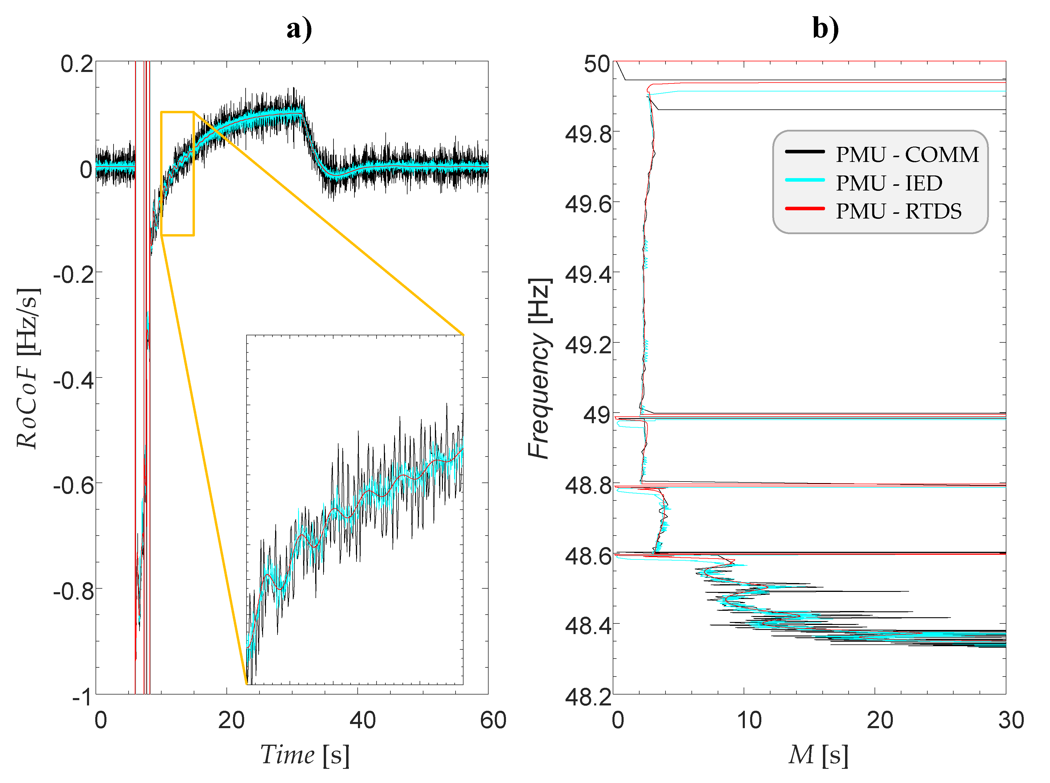
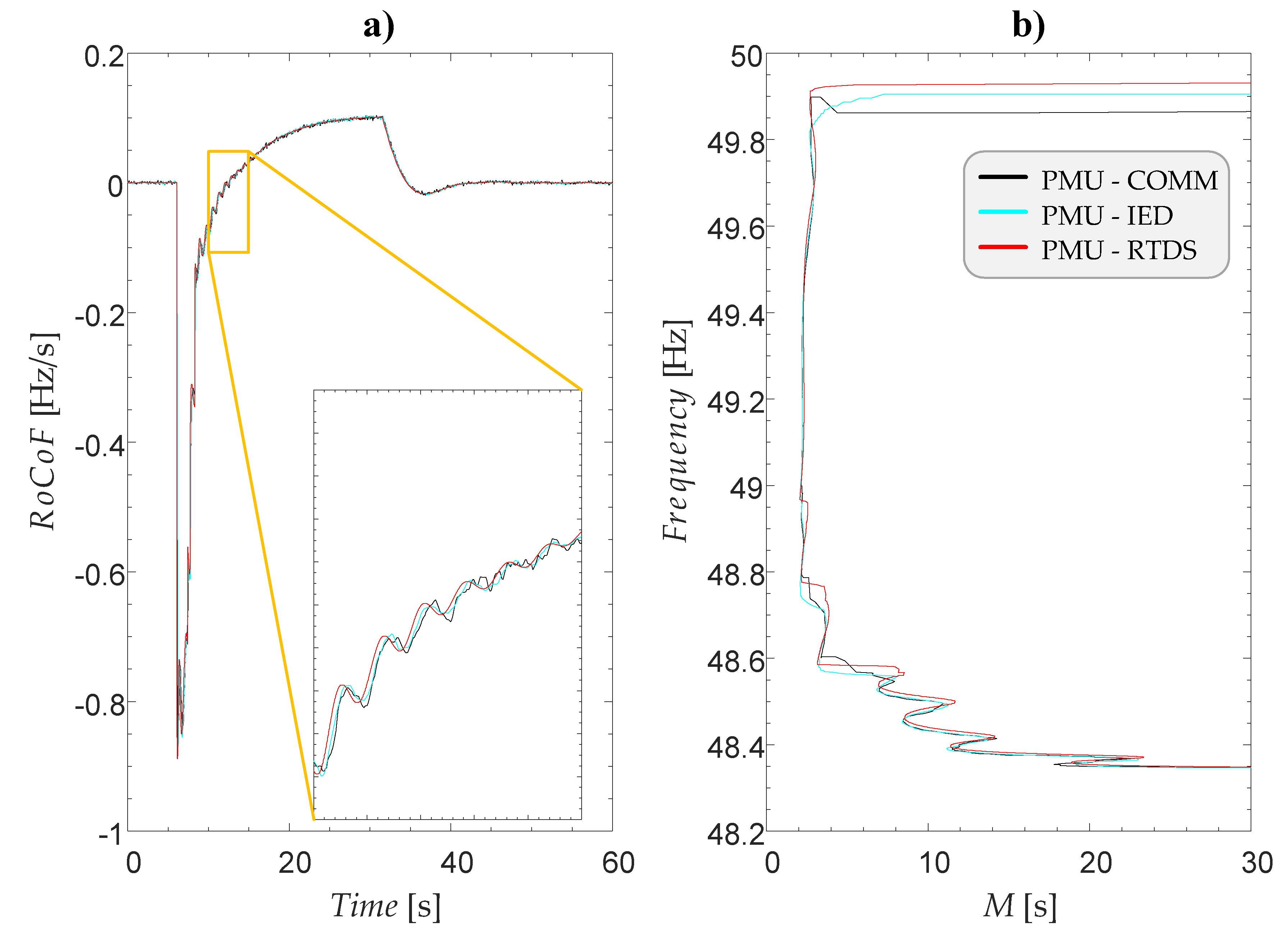
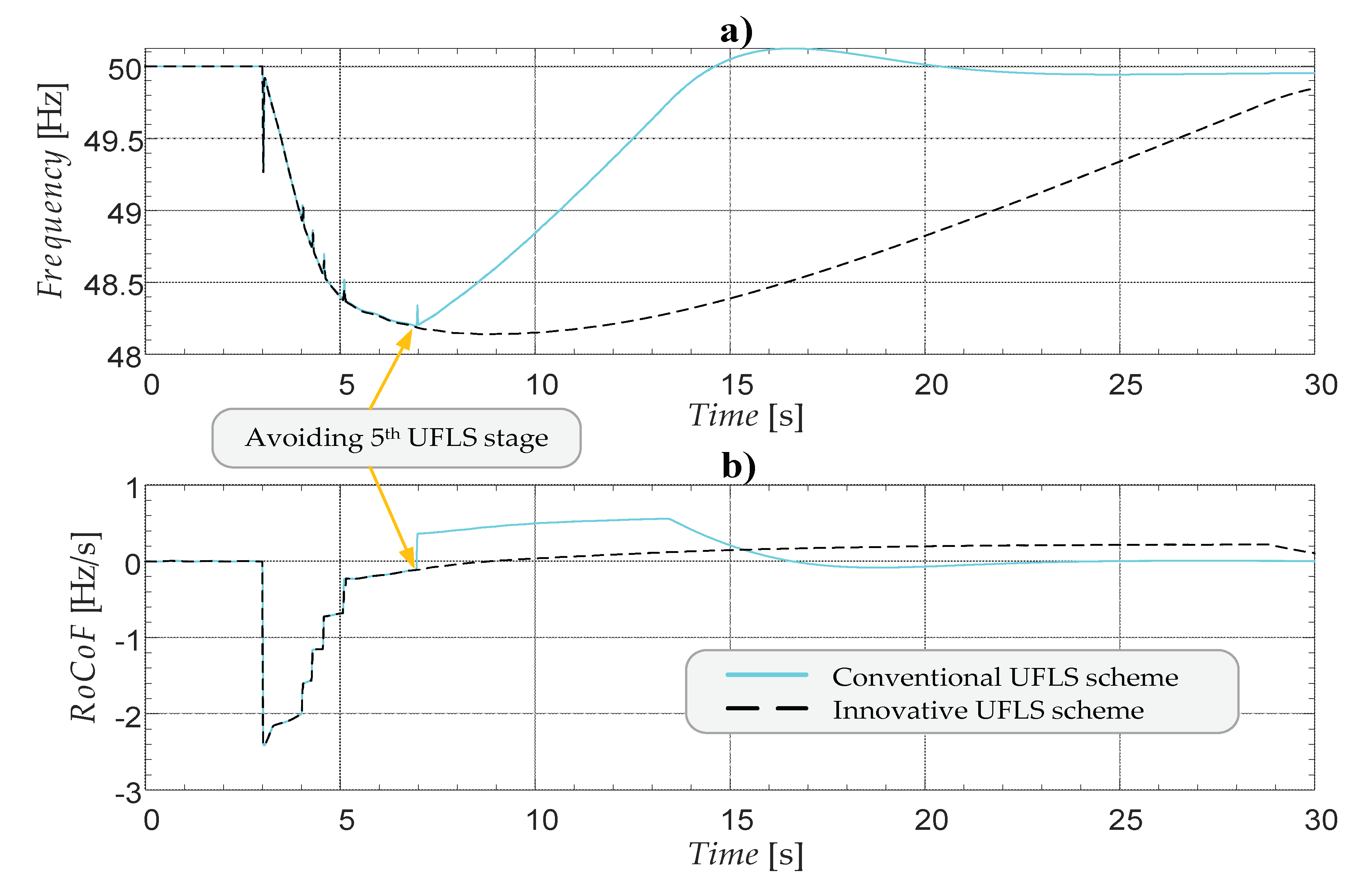
For simulated case no. 49, a time-domain response of the EPS frequency and RoCoF is depicted in Figure 11a and Figure 11b respectively. From observing the diagrams, it becomes evident that at the moment of reaching the frequency threshold of the fifth UFLS stage, innovative UFLS detects that there is still enough time available before frequency instability is endangered (M $\cong$ 8 s, Figure 12). As a result, the fifth UFLS stage is paused, which allows the frequency control to finish the frequency stabilization process by itself. If that was not the case, the fifth UFLS stage would have been triggered later on when the frequency would have approached the selected frequency stability limit f_LIM and, consequently, the M criterion of the fifth stage would have been triggered.

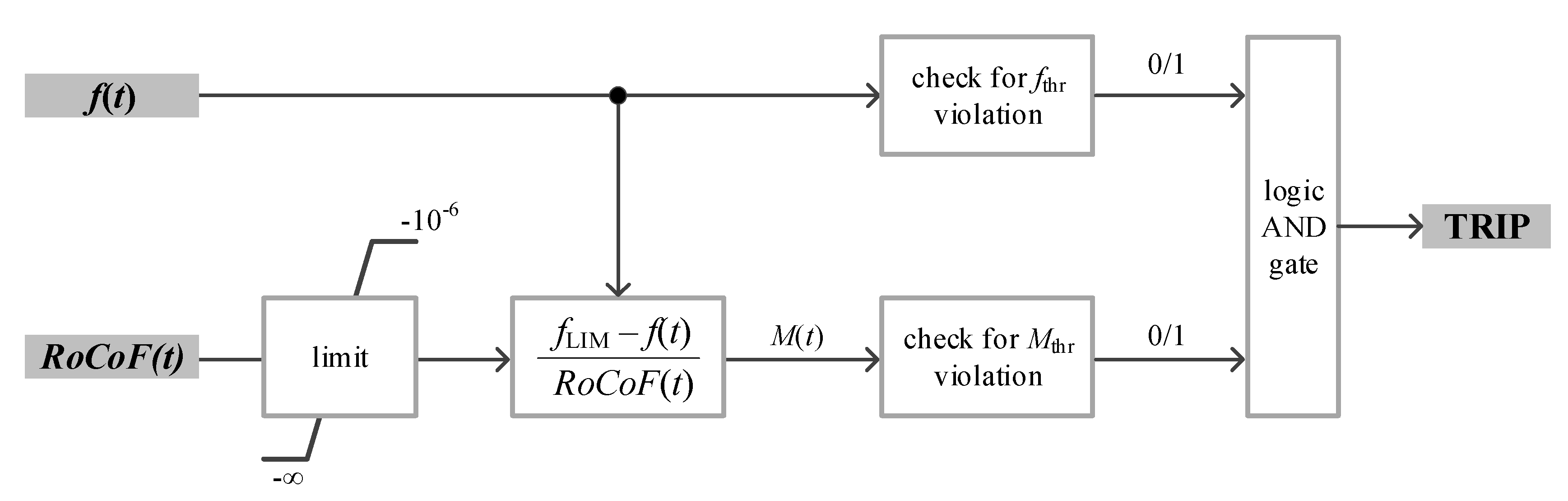
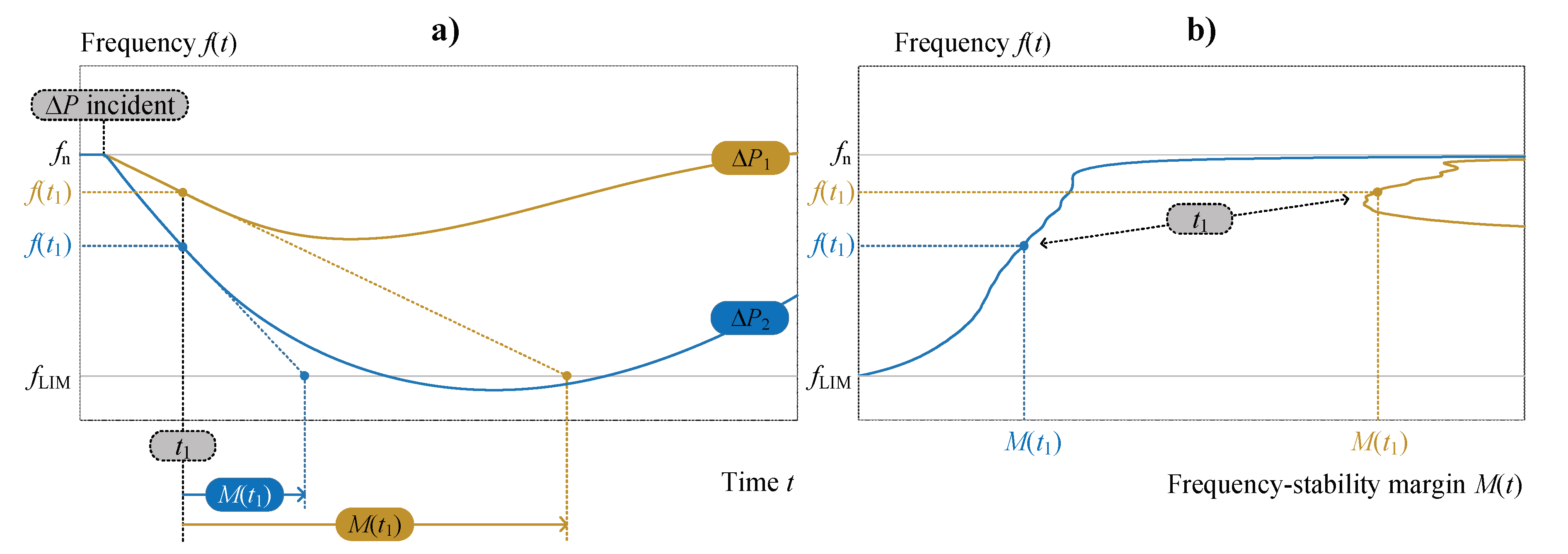
There is another essential thing that has to be discussed. When the frequency is decreasing with a significant RoCoF(t), a prompt triggering of UFLS is required since any additional time delay might be unacceptable. This is inherently achieved in conventional UFLS (triggering solely according to the frequency criterion f_thr) and it is vital to be aware that this is also the case with innovative UFLS. 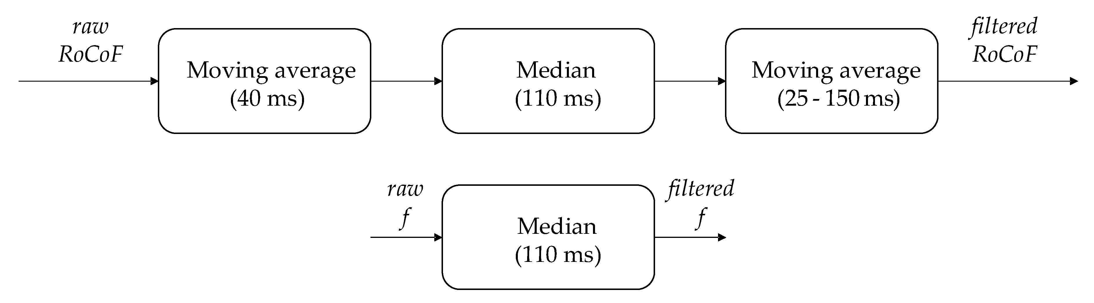The initial concern with the innovative UFLS scheme was related to extreme scenarios, in which the curve on the f(t)-M(t) plane is expected to make a rather abrupt jump from the upper right corner (steady-state conditions) to the upper left corner of the diagram once power imbalance appears. The delayed recognition of such critical conditions due to two additional moving average filters (Figure 7) could, therefore, translate into f_thr of a certain stage being violated before the corresponding M_thr. This would in turn be observed as shedding at lower frequency compared to a conventional UFLS scheme. However, our testing proved that even when dealing with an extreme initial RoCoF $(\cong$−10 Hz/s), the M_thr criterion is still violated sufficiently prior to the f_thr criterion. In

Table 2. Frequency values at which individual M_thr thresholds are violated (RoCoF = −10 Hz/s).

UFLS Stage Number	${\mathit{f}}_{\mathbf{t}\mathbf{h}\mathbf{r}}\left[\mathbf{Hz}\right]$	Frequency at Which Mthr Criterion Is Met [Hz]	Margin [Hz]
1.	49.0	49.4830	0.4830
2.	48.8	49.4830	0.6830
3.	48.6	49.4623	0.8623
4.	48.4	49.4623	1.0623
5.	48.2	49.4364	1.2364
6.	48.1	49.3415	1.2415

, the actual frequency at which the M_thr was met is given for each UFLS stage. Evidently, M criteria of all UFLS stages were met before the frequency even reached the f_thr value of the first UFLS stage (0.483 Hz margin in a worst-case scenario—see the last column in Table 2). This proves that the innovative UFLS scheme would respond to such an extreme event identically as the conventional scheme, with no additional time delay.

5. Conclusions

In the most common viewpoint of smart grids, the decentralization of electric power generation is usually accompanied by the centralization of protection functions. In this paper, we proved the concept of a RoCoF-based innovative UFLS which does not require centralization, yet still provides a high level of efficiency and flexibility. The main conclusion of this paper is that the innovative UFLS is deemed feasible and robust in practical applications. A proposed transition from conventional towards innovative UFLS is extremely simple; (i) an exceptionally simple logic based on RoCoF has to be incorporated in each under-frequency relay and (ii) a second criterion has to be added (parallel to the existing frequency threshold) for real-time monitoring. This new criterion is based on a patent-pending frequency stability margin calculated in real-time from the RoCoF and frequency values.

HIL simulations proved that innovative UFLS is feasible for real-world scenarios and that applying RoCoF does not affect its robustness in any of the tested conditions if the correct filtering techniques are selected. The main advantages of the innovative UFLS can be observed in moderate RoCoF conditions, being such from the very moment of a power deficit occurrence or decreased later on by UFLS intervention.

To summarize the main contributions of this research which all relate to the practical aspects of the implementation of an innovative UFLS scheme under test: (i) a multi-stage RoCoF filtering procedure that enables using RoCoF for local frequency stability margin calculation and monitoring in real-time for UFLS purposes. Filtering improves the resolution (linear filter stages) and filters out the anomalies (non-linear filter stage) in RoCoF measurements, (ii) a proof that despite RoCoF filtering, introduced time delays do not diminish the speed of UFLS operation during fast-occurring events (tested for −10 Hz/s) as long as RoCoF is used in an appropriate manner as suggested in [17], (iii) a proof that IEDs with specifications similar to the PMU can be used for UFLS, which decreases cost (i.e., using the same device for EPS observability and UFLS protection) and opens up numerous possibilities, including building business and market models for UFLS as a part of the end consumer response and other market opportunities related to Smart Grids, and (iv) a new criterion for comparison between several UFLS methods, being the remaining RoCoF after UFLS stops intervening.

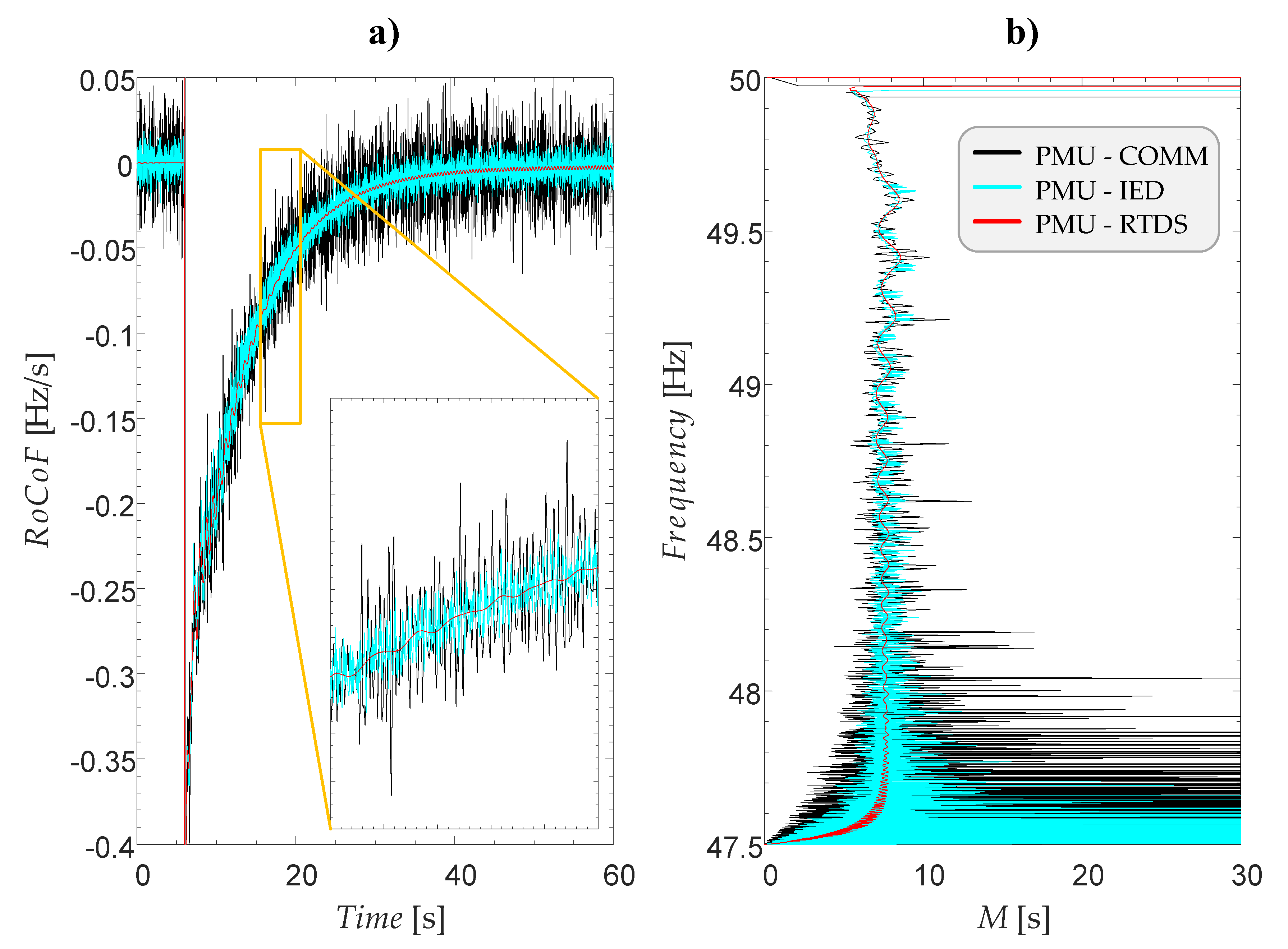
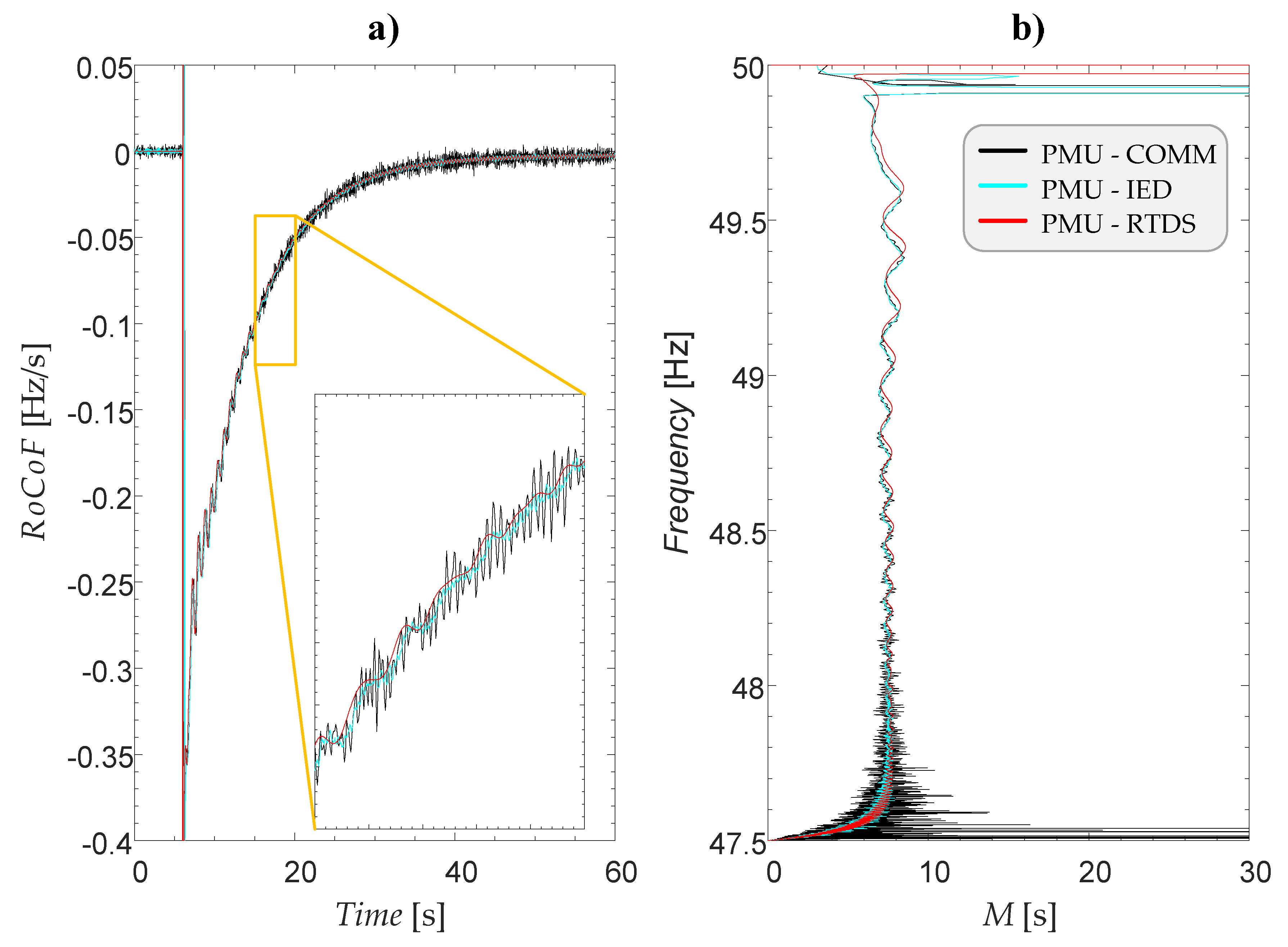
The analysis revealed that the diversity of IEDs (e.g., relays) and RoCoF-measuring techniques present in an EPS is beneficial to the UFLS method under test. Further optimization of RoCoF filtering is possible to reduce time delays, but one has to keep in mind that optimization, according to the noise requirements, has to be appropriately considered. Future work will be directed towards the development of the UFLS concept in which bulk load shedding is left to conventional UFLS, whereas handling the remaining power imbalance is left to smart devices (e.g., smart meters) located at end consumers and, therefore, widespread within the entire EPS.

6. Patents

This work is a subject to a pending International Patent Application No. PCT/EP2018/059048 filed on 9 April 2018.

References

1. H2020 Migrate. Available online: https://www.h2020-migrate.eu/ (accessed on 14 May 2020).
2. Winter, W.; Elkington, K.; Bareux, G.; Kostevc, J. Pushing the Limits: Europe’s New Grid: Innovative Tools to Combat Transmission Bottlenecks and Reduced Inertia. IEEE Power Energy. Mag. 2015, 13, 60–74. [Google Scholar] [CrossRef]
3. Anderson, P.M. Power System Control and Stability, 2nd ed.; Wiley-IEEE Press: Piscataway, NJ, USA, 2008; ISBN 978-0-471-23862-1. [Google Scholar]
4. Pulgar-Painemal, H.; Wang, Y.; Silva-Saravia, H. On Inertia Distribution, Inter-Area Oscillations and Location of Electronically-Interfaced Resources. IEEE Trans. Power Syst. 2018, 33, 995–1003. [Google Scholar] [CrossRef]
5. Bidram, A.; Davoudi, A. Hierarchical Structure of Microgrids Control System. IEEE Trans. Smart Grid 2012, 3, 1963–1976. [Google Scholar] [CrossRef]
6. Li, S.; Tang, F.; Shao, Y.; Liao, Q. Adaptive Under-Frequency Load Shedding Scheme in System Integrated with High Wind Power Penetration: Impacts and Improvements. Energies 2017, 10, 1331. [Google Scholar] [CrossRef] [Green Version]
7. Małkowski, R.; Nieznański, J. Underfrequency Load Shedding: An Innovative Algorithm Based on Fuzzy Logic. Energies 2020, 13, 1456. [Google Scholar] [CrossRef] [Green Version]
8. Sigrist, L. A UFLS Scheme for Small Isolated Power Systems Using Rate-of-Change of Frequency. IEEE Trans. Power Syst. 2015, 30, 2192–2193. [Google Scholar] [CrossRef]
9. Hong, Y.-Y.; Nguyen, M.-T. Multiobjective Multiscenario Under-Frequency Load Shedding in a Standalone Power System. IEEE Syst. J. 2020, 14, 2759–2769. [Google Scholar] [CrossRef]
10. Banijamali, S.S.; Amraee, T. Semi-Adaptive Setting of Under Frequency Load Shedding Relays Considering Credible Generation Outage Scenarios. IEEE Trans. Power Deliv. 2019, 34, 1098–1108. [Google Scholar] [CrossRef]
11. Potel, B.; Cadoux, F.; De Alvaro Garcia, L.; Debusschere, V. Clustering-based method for the feeder selection to improve the characteristics of load shedding. IET Smart Grid 2019, 2, 659–668. [Google Scholar] [CrossRef]
12. Shekari, T.; Gholami, A.; Aminifar, F.; Sanaye-Pasand, M. An Adaptive Wide-Area Load Shedding Scheme Incorporating Power System Real-Time Limitations. IEEE Syst. J. 2018, 12, 759–767. [Google Scholar] [CrossRef]
13. Zuo, Y.; Frigo, G.; Derviškadić, A.; Paolone, M. Impact of Synchrophasor Estimation Algorithms in ROCOF-Based Under-Frequency Load-Shedding. IEEE Trans. Power Syst. 2020, 35, 1305–1316. [Google Scholar] [CrossRef]
14. He, P.; Wen, B.; Wang, H. Decentralized Adaptive Under Frequency Load Shedding Scheme Based on Load Information. IEEE Access 2019, 7, 52007–52014. [Google Scholar] [CrossRef]
15. Tofis, Y.; Timotheou, S.; Kyriakides, E. Minimal Load Shedding Using the Swing Equation. IEEE Trans. Power Syst. 2017, 32, 2466–2467. [Google Scholar] [CrossRef]
16. Jallad, J.; Mekhilef, S.; Mokhlis, H.; Laghari, J.A. Improved UFLS with consideration of power deficit during shedding process and flexible load selection. IET Renew. Power Gener. 2018, 12, 565–575. [Google Scholar] [CrossRef]
17. Rudez, U.; Mihalic, R. RoCoF-based Improvement of Conventional Under-Frequency Load Shedding. In Proceedings of the 2019 IEEE Milan PowerTech, Milan, Italy, 23–27 June 2019; pp. 1–5. [Google Scholar]
18. Maglia, M.F.; Olama, M.M.; Ollis, B. Hardware-in-the-loop Testing of Signal Temporal Logic Frequency Control in a Microgrid. In Proceedings of the 2020 IEEE Power Energy Society Innovative Smart Grid Technologies Conference (ISGT), Washington, DC, USA, 17–20 February 2020; pp. 1–5. [Google Scholar]
19. SimTec—PSS SINCAL Platform. Available online: http://www.simtec-gmbh.at/sites_en/platform.asp (accessed on 15 June 2020).
20. Rudez, U.; Mihalic, R. Monitoring the First Frequency Derivative to Improve Adaptive Underfrequency Load-Shedding Schemes. IEEE Trans. Power Syst. 2011, 26, 839–846. [Google Scholar] [CrossRef]
21. IEEE/IEC Approved Draft International Standard—Measuring Relays and Protection Equipment—Part 118-1: Synchrophasor for Power System—Measurements; IEEE: Piscataway, NJ, USA, 1 January 2018; pp. 1–75. ISBN 978-1-5044-4682-2.
22. Eriksson, R.; Modig, N.; Elkington, K. Synthetic inertia versus fast frequency response: A definition. IET Renew. Power Gener. 2018, 12, 507–514. [Google Scholar] [CrossRef]
23. Smith, S.W. The Scientist & Engineer’s Guide to Digital Signal Processing, 1st ed.; California Technical Pub: San Diego, CA, USA, 1997; ISBN 978-0-9660176-3-2. [Google Scholar]
24. IEEE Standard for Synchrophasor Measurements for Power Systems. IEEE Std. C371181-2011; IEEE: Piscataway, NJ, USA, 28 December 2011; pp. 1–61. ISBN 978-0-7381-6811-1. [CrossRef]
25. IEEE Standard for Synchrophasor Data Transfer for Power Systems. IEEE Std C371182-2011; IEEE: Piscataway, NJ, USA, 28 December 2011; pp. 1–53. ISBN 978-0-7381-6813-5. [CrossRef]
26. RSCAD: Real-Time Simulation Software Package. Available online: http://knowledge.rtds.com/hc/en-us/articles/360046352893 (accessed on 16 June 2020).
27. ELES d.o.o. Sistemska Obratovalna Navodila Za Prenosni Sistem Električne Energije Republike Slovenije; ELES d.o.o.: Ljubljana, Slovenia, 2016. [Google Scholar]
28. Santos, A.Q.; Monaro, R.M.; Coury, D.V.; Oleskovicz, M. New scoring metric for load shedding in multi-control area systems. Transm. Distrib. IET Gener. 2017, 11, 1179–1186. [Google Scholar] [CrossRef]
29. Matthewman, S.; Byrd, H. Blackouts: A Sociology of Electrical Power Failure. Soc. Space 2013, 2, 31–55. [Google Scholar]
30. Sigrist, L.; Rouco, L.; Echavarren, F.M. A review of the state of the art of UFLS schemes for isolated power systems. Int. J. Electr. Power Energy Syst. 2018, 99, 525–539. [Google Scholar] [CrossRef]
Figure 1. EPS frequency f(t) response to different ΔP incidents (a) and the corresponding frequency versus frequency stability margin diagram (b).
Energies 13 03607 g001
Figure 2. A simplified logical diagram of the innovative UFLS process.
Energies 13 03607 g002
Figure 3. The RoCoF(t) report of three applied sources (PMU-IED, PMU-COMM and PMU-RTDS) after an RTDS simulation of an active power deficit (a) and a corresponding frequency versus frequency stability margin diagram (b).
Energies 13 03607 g003
Figure 4. The improvement in reported RoCoF(t) after applying a moving average filter to the PMU-IED and the PMU-COMM (a), and a corresponding frequency versus frequency stability margin diagram (b).
Energies 13 03607 g004
Figure 5. The RoCoF(t) report of three applied sources (PMU-IED, PMU-COMM and PMU-RTDS) after the RTDS simulation of an active power deficit and three UFLS interventions (a) and a corresponding frequency versus frequency stability margin diagram (b).
Energies 13 03607 g005
Figure 6. The improvement in reported RoCoF dynamics after applying a median filter to the PMU-IED and the PMU-COMM (a), a corresponding frequency versus frequency stability margin diagram (b).
Energies 13 03607 g006
Figure 7. The configuration of filtering applied to the reported frequency f and RoCoF.
Energies 13 03607 g007
Figure 8. A graphical representation of a real-time digital simulation setup.
Energies 13 03607 g008
Figure 9. A single-line diagram of a IEEE 9-bus test system [3], used for the RTDS HIL testing.
Energies 13 03607 g009
Figure 10. Overview of HIL results extracted from the entire set of 66 simulated cases; the total amount of disconnected consumption in percentages (a) and recorded RoCoF after the last UFLS intervention (b).
Energies 13 03607 g010
Figure 11. A time-domain response of the EPS frequency f(t) (a) and RoCoF(t) (b), corresponding to simulation case 49.
Energies 13 03607 g011
Figure 12. Frequency f(t) versus frequency stability margin M(t) diagram of simulation case 49.
Energies 13 03607 g012