Predictive Adaptive Filter for Reducing Total Harmonics Distortion in PV Systems

Abstract

This paper presents a new method for reducing the total harmonic distortion (THD) of photovoltaic (PV) systems by using an adaptive filter based on a predictive model. Instead of reducing the produced THD at each stage of the PV system, a one-step process is implemented at the end stage. The connection topology of the adaptive filter is similar to normal active and passive filters. The main difference is its ability to adjust the filtering coefficients while others cannot. The proposed method is applied to a single-phase standalone PV system by adopting least mean square (LMS), normalized LMS (NLMS) and leaky LMS algorithms to verify the validity of the proposed method. Various values of filter length and step size are evaluated, and results indicate that the proposed method can reduce THD in the current signal of the PV system significantly by using all of the mentioned algorithms. Different step sizes and filter lengths directly influence the effectiveness of the THD reduction, with small step sizes and long filters being the most effective. Amongst the algorithms, NLMS reduces THD the most, and LMS reaches the peak current value the fastest.

1. Background

Photovoltaics (PV) is one of the most popular energy sources and has been used widely in the last decade due to the increasing demands on alternative clean energy sources. A PV system generally consists of panels to convert photonic power into electricity, DC–DC converters to keep the output voltage stable at certain levels and DC–AC converters to make the power useable in homes. PV systems can be classified into two types, namely, standalone and grid-connected, depending on system application [1]. Standalone PV systems are further classified into those with and without a battery energy storage system to supply AC and DC power, respectively. Unlike the fourth section of a PV system, which describes the manner through which the PV system delivers power to consumers, the first three sections (PV panels, DC–DC converters and DC–AC converters) are common to all types of PV systems.

The solar power delivered to customers is usually contaminated with high levels of distortion due to different factors, such as irradiance fluctuation, temperature uncertainty and frequent switching of converter and inverter parts. The total harmonic distortion (THD) index is the most common means to determine the amount of distortion in a signal. THD is defined as the ratio between the total power accounted for by harmonics and the main power of the signal. A high level of THD affects the performance of the PV system in different ways, including heating, disoperation of electronic equipment, disruption of protective relays and communication interference [2,3,4]. THD in PV systems is more complicated than in other energy systems because it is an accumulated problem from each part of the system, and it occurs not only due to nonlinear loads.

The harmonic distortion generated in a PV system is a consequence of intrinsic and extrinsic effects. Intrinsic harmonic distortions include converter and inverter deficiencies, such as component and control loop nonlinearities, limited pulse-width modulation (PWM) resolution and measurement inaccuracies. Meanwhile, extrinsic harmonic distortion is a result of a connection to a weak and distorted electrical grid. A distorted voltage in the inverter control system acts like a disturbance by the inverter [5,6].

Several factors affect the power quality of PV inverter output current. Solar irradiance level is a key factor that increases current THD and reactive power levels. A low irradiance level (e.g., sunrise, sunset and cloudy days) increases the THD of the output current, but it is drastically reduced as the output active power of the PV inverter reaches its nominal value. The use of power converters to interface between PV systems and the power grid causes harmonic distortion in the output signal. However, this effect is less severe than the harmonics generated by an unstable irradiance level and temperature [7].

Considering this background, several studies have attempted to reduce THD levels, and the presented approaches can be classified into THD reduction at the DC and AC sides, as shown in Figure 1. Using maximum power point tracking (MPPT) algorithms and adopting different types of DC–DC converters are the two main techniques for THD reduction at the DC side. Utilizing various DC–AC inverters and using passive or active filters are the two main approaches for THD reduction at the AC side. Various MPPT techniques have also been adopted to reduce the THD of output power signals in the beginning of a PV system [8,9,10,11]. Many new topologies and control strategies including the use of adaptive control algorithms for the implementation of adaptive modular inverters [12,13] have been used to reduce THD in the converter and inverter sections of PV systems [14,15], and active and passive filters have been employed to reduce THD at the customer side of PV systems [16,17]. The development of these strategies is elucidated in the next section.

2. Literature Review

The purpose of MPPT is to ensure that a PV system extracts the maximum solar power in a steady and low-THD manner [8,11]. MPPT techniques can be classified into two main categories: classical and modern [19]. The perturbation and observation (P+O) method is the most popular MPPT technique for PV systems due to its simplicity. Steady precision, double tracking speed and efficient energy conversion are amongst the many benefits of using the P+O algorithm [20]. The algorithm is also easier to program and implement compared with other algorithms [19]. A modified version of P+O has been developed to predict the output power of PV arrays [20].

The hill climbing (HC) algorithm is similar to the P+O method; instead of being applied to voltage, perturbation is applied to the duty cycle of the DC–DC converter, and the increase in the duty cycle automatically leads to an increase in output power [19,21]. P+O and HC methods sometimes lead to misjudgement and oscillation around the maximum power point, thereby decreasing the efficiency of the PV system [19,20]. Hence, [22] introduced HC with an adaptive perturbation size, which can be adjusted only during the tracking process. In [23,24], a new version of adaptive HC was developed. Other techniques, such as fractional open-circuit voltage to short-circuit current ($V_{oc}\mathsf{/}{I}_{sc}$) [25,26,27], ripple correlation control (RCC) [28,29], current sweep strategy [30] and linear current control strategy [31] have also been used. Modern MPPT approaches, such as artificial neural networks (ANN), fuzzy logic control (FLC) and metaheuristics [32,33,34], are likewise available. These techniques have been used with P+O [35,36,37] and HC [19,38] to obtain efficient MPPT strategies. The metaheuristic method is the most advanced MPPT algorithm. It has been utilised to solve the optimisation problems that arise in PV systems due to the process of finding the maximum power point [19]. Recent studies have adopted metaheuristic algorithms, including particle swarm optimisation (PSO) [39,40,41], artificial bee colony (ABC) [42] and genetic algorithms (GA) [43]. Metaheuristic optimisation algorithms are efficient because of their system independency, effective performance and absence of oscillation around the maximum power point [19]. However, the performance of MPPT techniques is easily affected by partial shading of the sun by overhead clouds, which potentially reduce the power output by up to 25% [9,44]. Such fluctuations in power generate harmonics in the output power signal.

The THD of a PV system can also be reduced by decreasing the harmonics generated in the converter and inverter sections of the system. Studies that focused on this area have presented different DC–DC converter topologies, such as buck, boost, buck–boost, Cuk, single-ended primary-inductor converter and flyback converter [45,46,47,48]. These topologies function as switching mode regulators to control and convert the DC output into suitable voltage levels [46], which depend heavily on the switching frequency of the PWM control signal [49,50]. All of the presented topologies of DC–DC converters reduce the generated THD by maintaining the output DC voltage at certain levels. Amongst these topologies, the buck–boost converter is the most widely used, due to its efficient capability to maintain the output DC signal at a certain level, which in turn decreases THD. Several studies have been conducted in this area due to the frequent switching nature of DC–AC inverters and their undesirably high level of harmonics [51]. Various inverters and control algorithms have been explored to integrate PV arrays into grids [52]. The output signal from these inverters can be either single or three-phase, and the magnitude range may vary; however, the frequencies are typically 50, 60 and 400 Hz [53,54]. Common types of inverters are either single-phase, three-phase or multilevel [55,56,57]. Using several active and passive filters might push the PV system into the resonance region of the S-plane if many inductors or capacitors are used, thereby reducing signal stability and making the circuit bulky [18]. In addition to the drawbacks of the mentioned techniques, these techniques are only applicable to a specific part of the PV system. Several techniques usually need to be combined to reduce the accumulated THD, which complicates the PV system.

For these reasons, a simple filtering technique, preferably one that can be applied at the end of the system just before the load, is needed, so that the unwanted harmonics that accumulate throughout the various stages of the PV system can be eliminated without complicating the system’s design structure as other methods do. Although the adaptive−selective harmonic elimination (ASHE) proposed by Blasko et al. [58,59] for DC–AC inverters does not fit the mentioned criteria, it still provides insights into potential solutions. ASHE is based on one of the common filtering techniques used in communication and signal processing, namely, adaptive noise cancellation (ANC). Figure 2 shows that the inputs of the noise cancellation block diagram are the primary signal tainted with an unknown amount of noise ($s_j+n_j$) and the reference signal ($n^{\prime }$), which is an estimation of the noise in the primary signal. The output of the adaptive filter is computed by multiplying the reference signal with the filter weight, and it is then subtracted from the primary input to generate the error signal, which is also the output signal of the control system. The filter weight is adjusted based on the error signal, and the process is repeated until the error is minimised to a desirable level.

In the proposed ASHE, the third harmonic of the primary signal is used as the reference signal because it is the most dominant. However, this usage is inapplicable to the PV system because this system has multiple sources of harmonics generated from solar radiation and temperature fluctuations and multiple converter and inverter switching instances throughout the various stages of the PV system. This feature makes the analysis of signal frequency and amplitude difficult, and identifying the most dominant harmonic becomes impossible. The third harmonic is targeted in ASHE because it is feasible to examine the harmonic’s frequency and amplitude due to it having only a single source of input.

In addition to ANC, three other standard adaptive filters are used, and they are system identification, inverse modelling and system prediction [60,61]. Only noise cancellation and system prediction (Figure 3) adaptive filters have been proven useful for noise reduction and signal enhancement, with successful cases reported in speech and signal processing applications [59,62,63]. Furthermore, the noise cancellation adaptive filter is unsuitable for use in the PV system. Therefore, this study proposes the utilisation of the system prediction adaptive filter to reduce the THD of the PV system. The proposed method does not alter or complicate the original design structure of the system and only needs to be applied once before being delivered to consumers.

3. Methodology

Unlike the noise cancellation model, the proposed system prediction adaptive filter does not require an external source as the reference signal. Instead, a delayed version of the primary input serves as the reference signal. The output signal is obtained immediately from the filtered signal instead of from the subtraction, as shown in the noise cancellation block diagram. The common algorithms used to determine the filter’s weight with minimum error are based on least mean square (LMS), normalised LMS (NLMS) and leaky LMS (LLMS) [60,61,64]. These algorithms are used and compared in this work.

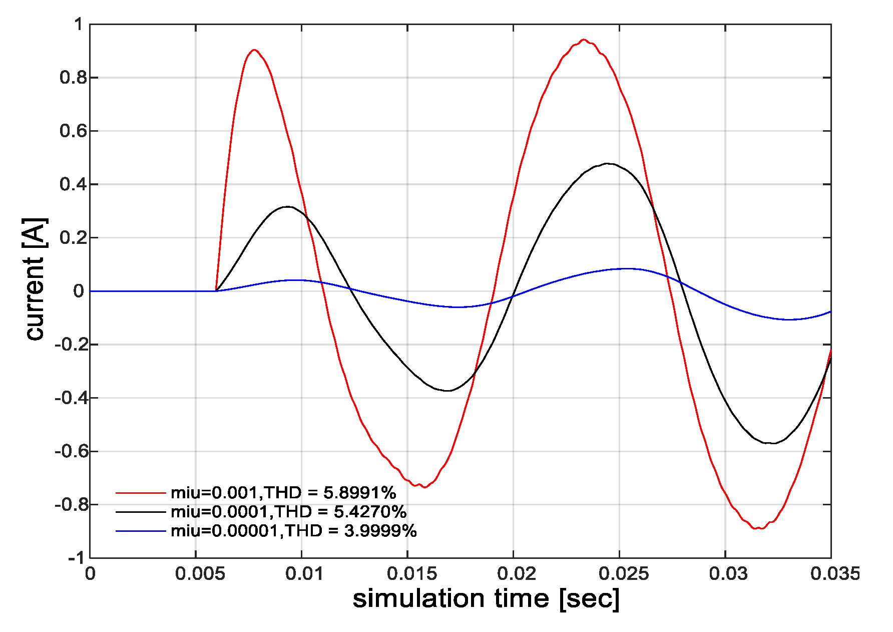
3.1. LMS Algorithm

LMS, the most common algorithm for adaptive filtering, consists of the following steps: (1) computing the output of the adaptive filter produced by a group of tap inputs, (2) generating an estimated error by comparing the output of the filter with the desired signal and (3) using the error signal to adjust the tap weights [60,61]. Selecting the proper step size of the iteration affects the stability and convergence speed of the LMS algorithm.

In the LMS algorithm, the cost function is defined as the mean square error between the estimated output and the actual one. The weights, error and output equations of the LMS algorithm are derived as follows [61].

Given an input $M\times M$ matrix, the $\mathit{X}\left(n\right)$ of the adaptive filter is

$$\mathit{X}\left(n\right)=\left[x\left(n\right),x\left(n-1\right),\dots ,x\left(n-M+1\right)\right]$$

(1)

where $M$ is the filter taps and $n$ is the current input sample. The output, $\overrightarrow{\mathit{Y}\left(n\right)}$, of the adaptive filter is

$$\mathit{Y}\left(n\right)=\left[y\left(n\right),y\left(n-1\right),\dots ,y\left(N-M+1\right)\right]=\mathit{X}\left(n\right)\mathit{W}{\left(n\right)}^T$$

(2)

where $y\left(n\right)$ is the output vector at time sample $n$ and $\mathit{W}\left(n\right)$ is the weight matrix, derived as

$$\mathit{W}\left(n\right)={\left[w\left(0\right),w\left(1\right),\dots ,w\left(M-1\right)\right]}^T$$

(3)

LMS uses the steepest descent method to find the filter weights that minimize the cost function $C\left(n\right)$. Moreover, $C\left(n\right)$ is the expected value of the square of the error signal, e$\left(n\right)$, which in turn is the difference between the desired output, $d\left(n\right)$, and the actual output, $y\left(n\right)$.

$$\mathit{e}\left(n\right)={\left[e\left(n\right),e\left(n-1\right),\dots ,e\left(n-M+1\right)\right]}^T$$

(4)

$$\mathit{d}\left(n\right)={\left[d\left(n\right),d\left(n-1\right),\dots ,d\left(n-M+1\right)\right]}^T$$

(5)

The cost function is defined as follows:

$$C\left(n\right)=E[{\left|\mathit{e}\left(n\right)\right|}^2]$$

(6)

where $E$ is the expected value. Using the partial derivatives with respect to the individual filter weight based on the steepest descent method to find the minimum value of the error signal leads to the following [61]:

$${\nabla }_{w}C\left(n\right)={\nabla }_{w}E[{\left|\mathit{e}\left(n\right)\right|}^2]=2\mathit{e}\left(n\right)\frac{\partial \mathit{e}\left(n\right)}{\partial w}$$

(7)

We also consider the following:

$$\mathit{e}\left(n\right)=\mathit{d}\left(n\right)-\mathit{X}\left(n\right)\mathit{W}{\left(n\right)}^T$$

(8)

which produces

$$\frac{\partial \mathit{e}\left(n\right)}{\partial w}=-\mathit{X}\left(n\right)$$

(9)

Substituting Equation (9) into Equation (7) produces

$${\nabla }_{w}C\left(n\right)=2\mathit{e}\left(n\right)\ast -\mathit{X}\left(n\right)$$

(10)

which represents the variation in the weight equation required to yield the minimum value of the cost function. On this basis, the weight update equation can be written as

$$\mathit{W}\left(n+1\right)=\mathit{W}\left(n\right)+\frac{\mu }{2}\ast 2\ast \mathit{e}\left(n\right)\ast \mathit{X}\left(n\right)$$

(11)

where $\mu$ is the step size. Equation (11) describes the relationship between the current and next weight vector.

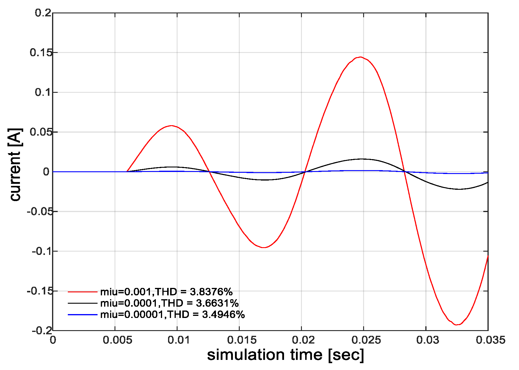
3.2. NLMS Algorithm

The adaptive filter’s length and the signal power might affect the stability, convergence and steady state behaviour of the LMS algorithm. NLMS overcomes these problems by normalising the input power. In NLMS, all of the equations presented previously are applicable, except for the weight update equation. Instead, the following is used [61]:

$$\mathit{W}\left(n+1\right)=\mathit{W}\left(n\right)+\frac{\mu }{\epsilon +\Vert \mathit{X}{\left(n\right)}^2\Vert }\ast \mathit{e}\left(n\right)\ast \mathit{X}\left(n\right)$$

(12)

where $\Vert \mathit{X}{\left(n\right)\Vert }^2=\mathit{X}{\left(n\right)}^H\ast \mathit{X}\left(n\right)$ is the normalisation factor, with H denoting the complex conjugate transposed and $\epsilon$ the regularisation size.

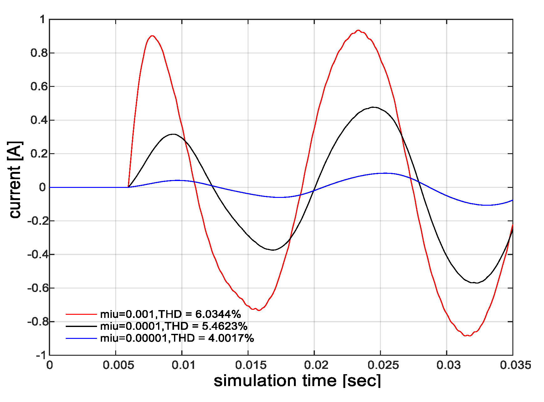
3.3. LLMS Algorithm

To ensure the stability and increase the convergence speed of the LMS algorithm without specifying and consequently restricting the learning rate of the step size, LLMS is used instead [64]. Its filter weight is updated as follows, with all other parts remaining the same:

$$\mathit{W}\left(n+1\right)=\left(1-\mu \ast \eta \right)\mathit{W}\left(n\right)+\mu \ast \mathit{e}\left(n\right)\ast \mathit{X}\left(n\right)$$

(13)

where $\eta$ is the leaky factor, which is a very small positive number ($\eta$ << 1).

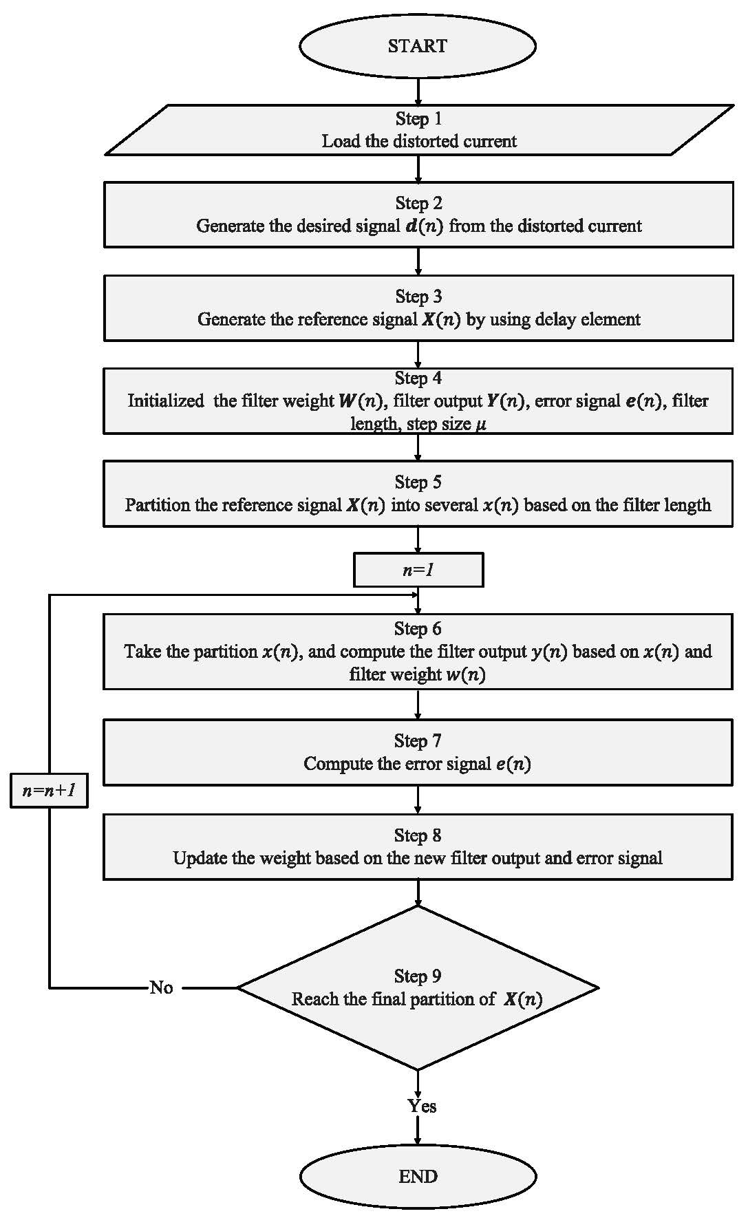
3.4. THD Filtering Process

The general block diagram of the PV system is shown in Figure 4. To improve the quality of the output signal and reduce the accumulated THD, this paper proposes the use of an adaptive filter just before the load or grid, as shown in Figure 5. The working principle of the adaptive filter in this connection topology is similar to normal active and passive filters. The main difference will be in how the adaptive filter can adjust its filtering coefficients while other filters cannot. The adaptive filter processes the distorted current signal before delivering it to the load based on an adaptive prediction model. The distorted output current signal of the PV system is cleaned using the proposed block diagram by applying the three algorithms mentioned in Section 3. The algorithms’ results are compared afterwards. The flowchart of the THD reduction procedure is shown in Figure 6 and described below.

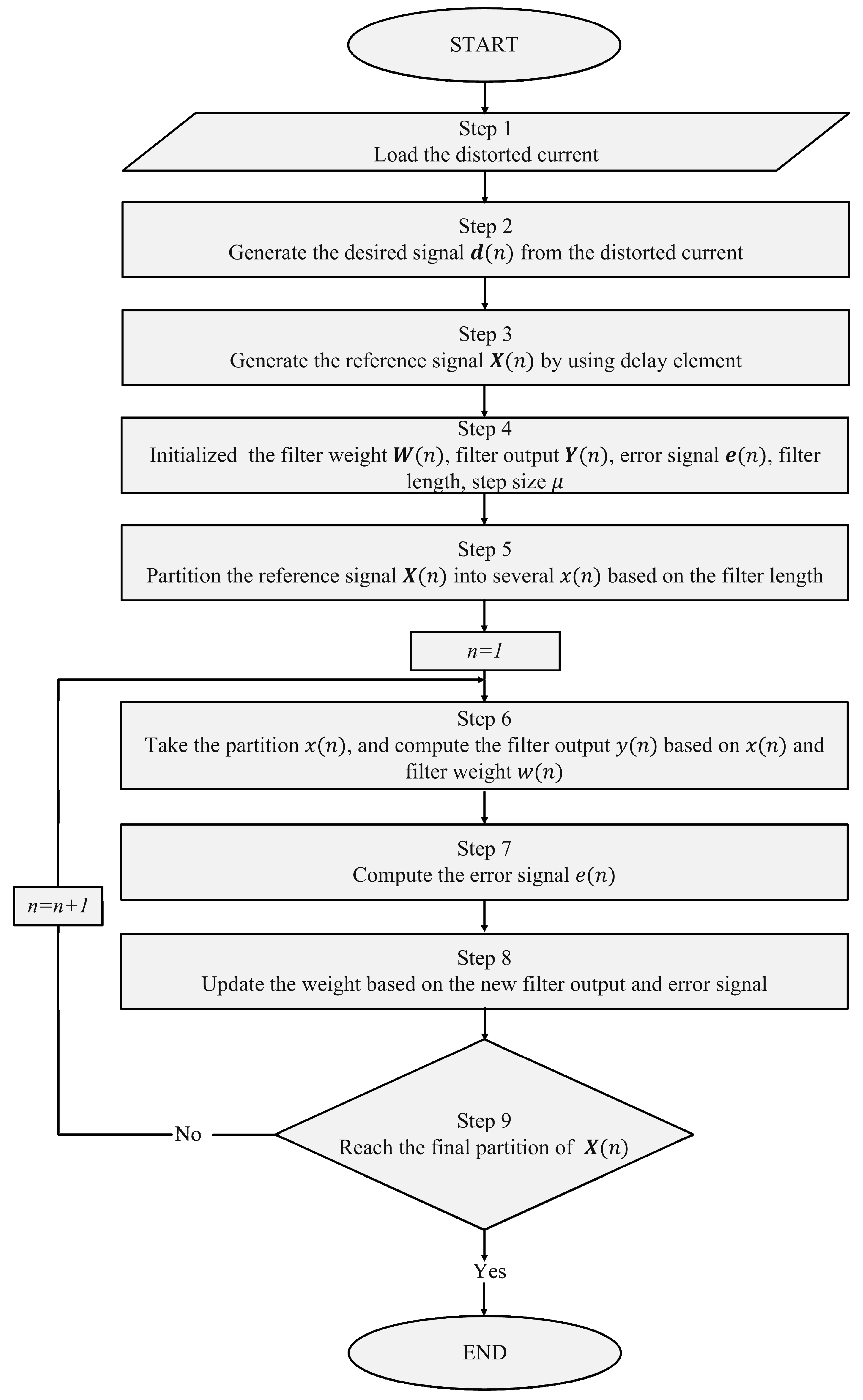
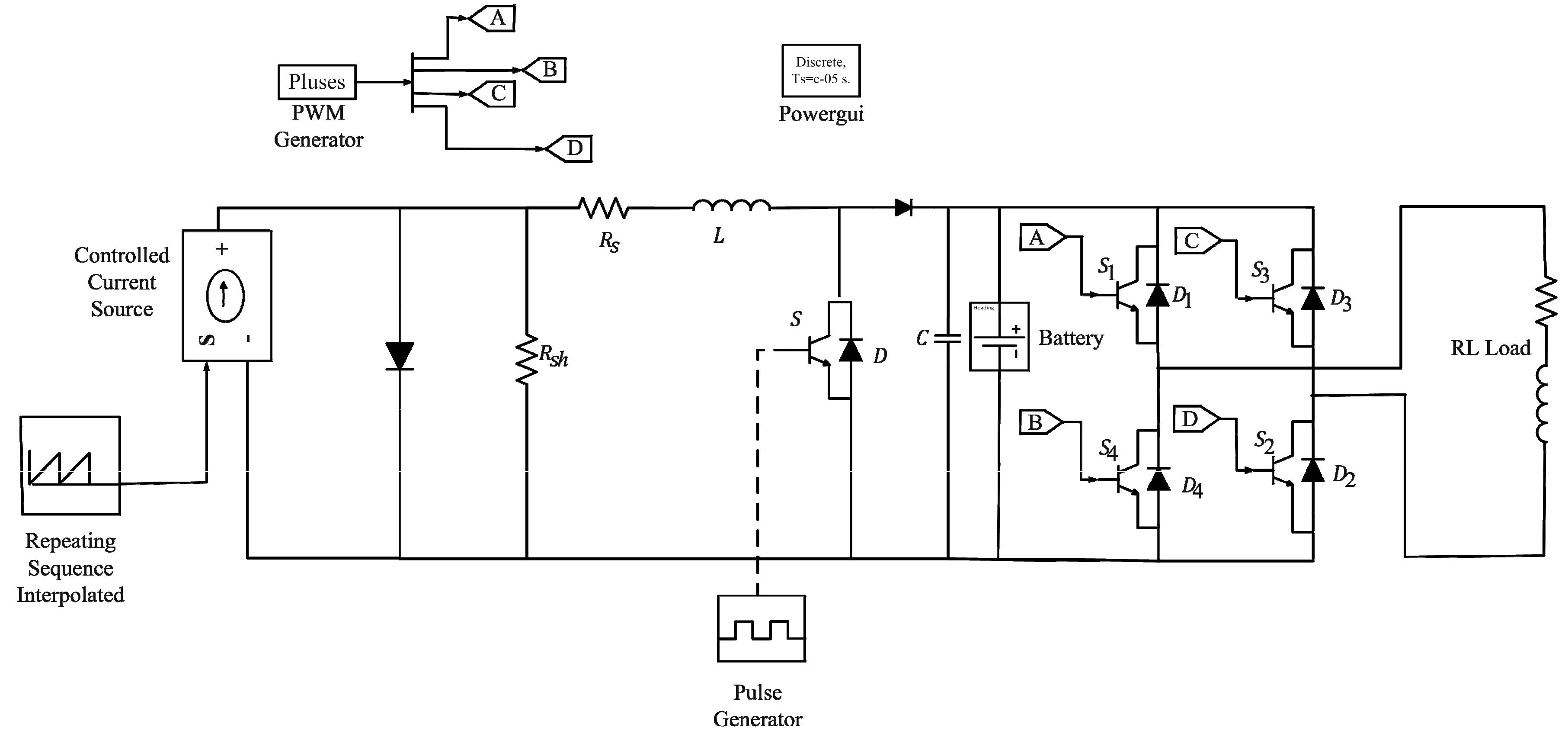
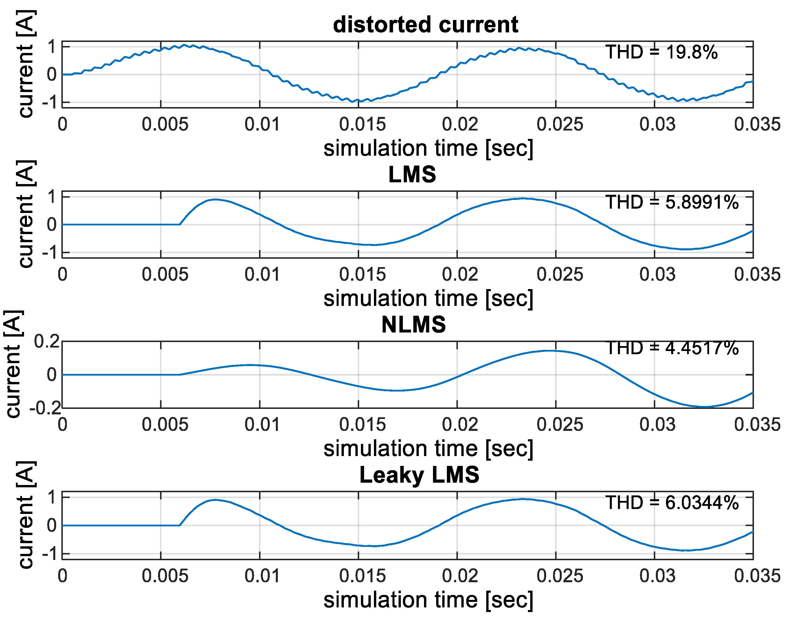
• Step 1: The distorted current signal from the output of the PV system shown in Figure 6 is loaded. The distorted current serves as the primary signal of the adaptive filter.
• Step 2: The desired signal $\mathit{d}\left(n\right)$ is generated from the primary signal by initialising $\mathit{d}\left(n\right)$ as the primary signal.
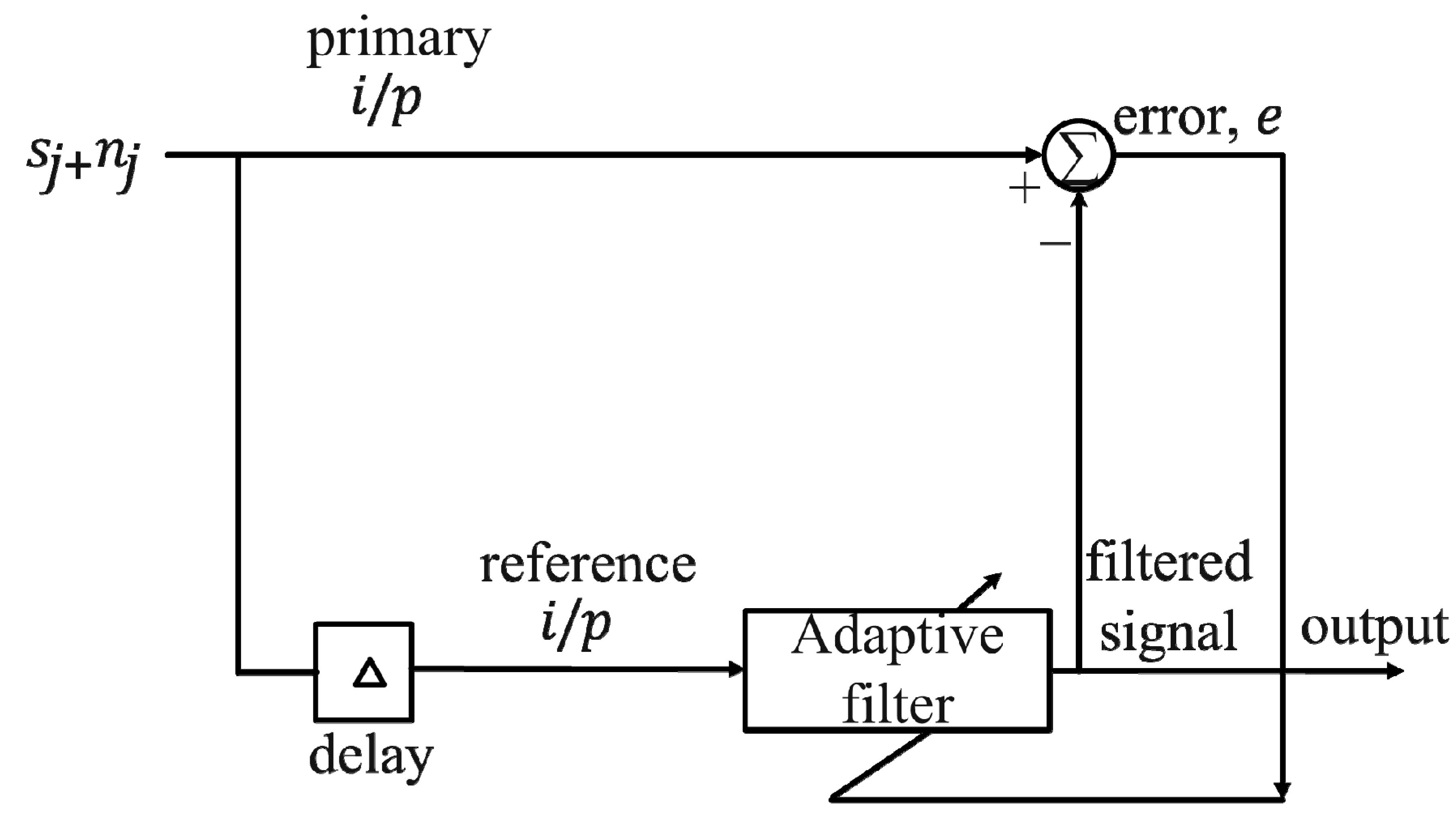
• Step 3: The reference signal is generated from the desired signal by using a unit time delay, i.e., $\mathit{X}\left(n\right)=\mathit{d}\left(n-1\right)$.
• Step 4: The initial values of filter length $M$, filter weight $\mathit{W}\left(n\right)$, filter output $\mathit{Y}\left(n\right)$, error signal $\mathit{e}\left(n\right)$ and step size $\mu$ are set up.
• Step 5: The reference signal $\mathit{X}\left(n\right)$ is divided into several partitions $x\left(n\right)$ based on the size of the signal and adaptive filter. For example, if the reference signal has 1000 elements and the filter length is $M=20$, then the number of the partitions will be 50 ($1000/20=50$).
• Step 6: The filter output $y\left(n\right)$ is computed by multiplying $x\left(n\right)$ with the filter weight, where $n$ is the range of all partitions.
• Step 7: The error signal $e\left(n\right)=d\left(n\right)-y\left(n\right)$ is computed.
• Step 8: The filter weight is updated with the new values of $e\left(n\right)$ and $x\left(n\right)$ based on Equation (11), (12) or (13), depending on whether the LMS, NLMS or LLMS is used, respectively.
• Step 9: Steps 6–8 are repeated until the entire reference signal is covered. The level of THD before and after applying the adaptive filter is determined as follows:

  $$\mathrm{THD}(\%)=100\%\ast \sqrt{\frac{i_2^2+i_3^2+i_4^2+\dots \dots +i_n^2}{i_1^2}}$$

  (14)

  where $i_n$ is the current root mean square and n is the harmonic order.

4. Results and Discussion

A single-phase standalone PV system was built in MATLAB Simulink, as shown in Figure 7. The PV model consists of a photocurrent source, a diode and resistors. The photocurrent source is the solar irradiance, which varies from $0\mathrm{W}/{\mathrm{m}}^2$ during nighttime to $1000\mathrm{W}/{\mathrm{m}}^2$ during the peak hours of daytime. The effects of temperature on PV efficiency are disregarded. The values of series and parallel resistances are 0.01 Ω and 10 KΩ, respectively, which are common in PV systems. The PV model is connected to a DC–DC converter to stabilize the output voltage, then to the DC–AC inverter before supplying power to the RL load, which is the most common load characteristic. PWM generators are used to control the converter and inverter circuits. The peak current setting is 1 A.

The distorted output current signal of the PV system is filtered based on the algorithms and filtering process described in Section 3. The results obtained based on step size $\mu =0.001$ and filter length $M=30$ are shown in Figure 8. All of the filtered signals are visibly smoother than before, and the THD level is reduced in each case. The THD of the current signal is 19.8% before filtering and successfully reduced to approximately 5.9%, 3.8% and 6.0% after filtering using LMS, NLMS and LLMS algorithms, respectively, proving that the NLMS algorithm is superior to the others.

Various filter step sizes and their effects on filtering are explored whilst maintaining filter length $M=30$. The results are shown in Figure 9, Figure 10 and Figure 11 for LMS, NLMS and LLMS algorithms. As shown in Figure 9, the THD based on the LMS algorithm is approximately 5.9% when $\mu =0.001$ (similar to the result in Figure 8), but it is reduced to approximately 5.4% and 4.0% when the step size decreases to $\mu =0.0001$ and $\mu =0.00001$, respectively. Repeating the same investigation using the NLMS algorithm in Figure 10 shows that the THD level decreases from approximately 3.9% to 3.6% and 3.5%. In the LLMS algorithm’s case in Figure 11, THD is reduced from 6% to 5.4% and 4.0%. These results are summarized in

Table 1. THD based on various step sizes with fixed filter length $M=30$.

Step Size	LMS	NLMS	LLMS
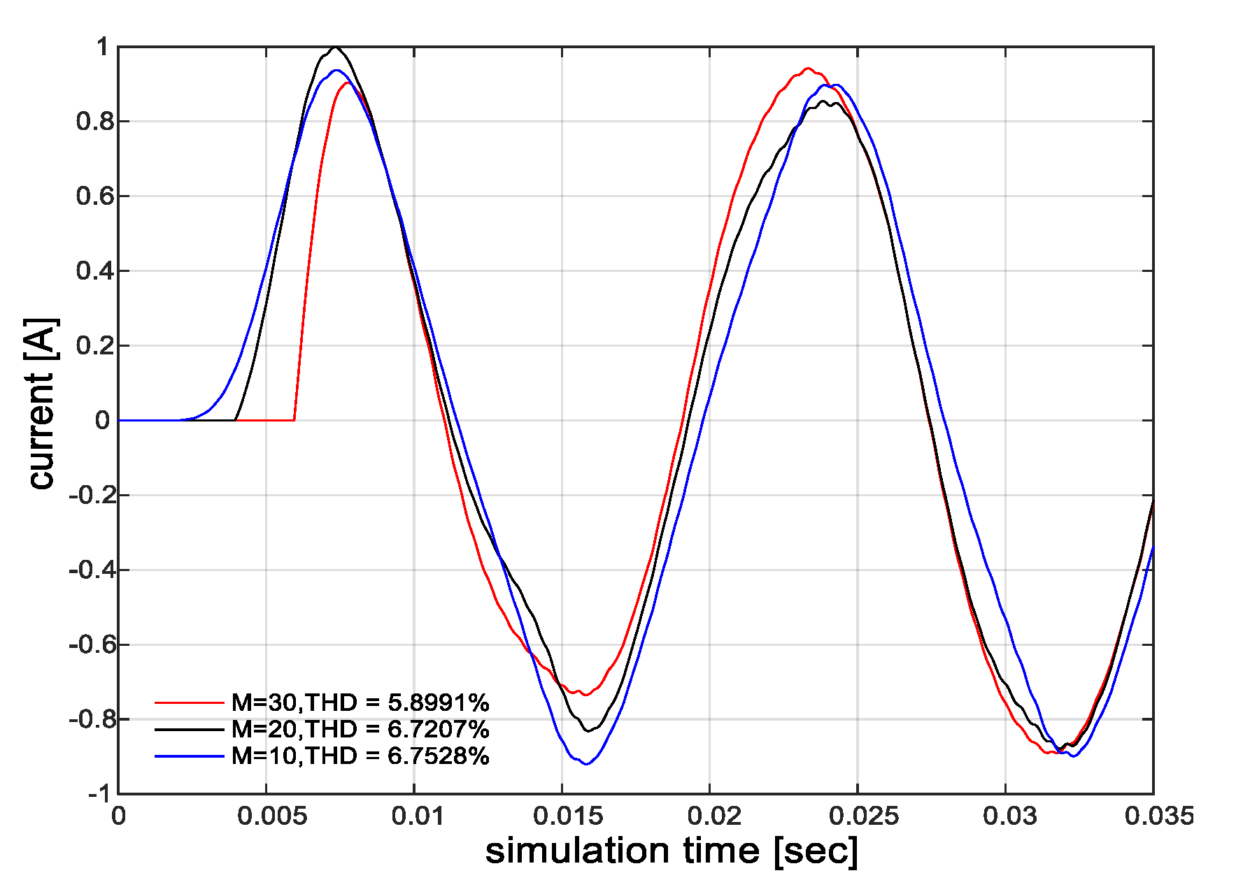
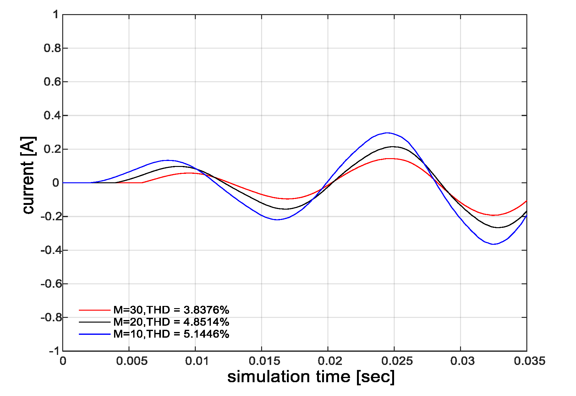
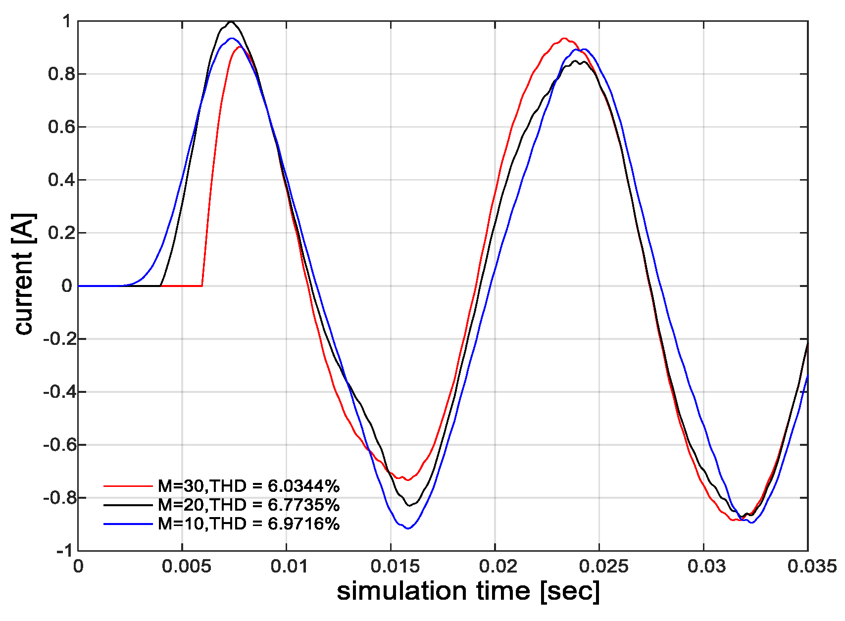
μ = 0.001	5.8991%	3.8376%	6.0344%
μ = 0.0001	5.4270%	3.6631%	5.4623%
μ = 0.00001	3.9999%	3.4946%	4.0017%

. The effects of filter length are also studied with the three algorithms whilst maintaining step size $\mu =0.001$ (Figure 12, Figure 13 and Figure 14). These results indicate that as the filter length decreases from $M=30$ to $M=10$ the THD level increases from 5.9%, 3.9% and 6.0% to 6.8%, 5.1% and 7.0% for LMS, NLMS and LLMS algorithms, respectively, indicating that a long filter is effective in reducing THD. The results are summarised in

Table 2. THD based on various filter lengths with fixed step size $\mu =0.001$.

Filter Length	LMS	NLMS	LLMS
$M=10$	6.7528%	5.1446%	6.9716%
$M=20$	6.7207%	4.8514%	6.7735%
$M=30$	5.8991%	3.8376%	6.0344%

.

The times taken by each algorithm to reach the peak 1A current based on various step sizes and filter length settings are also compared, and the results are given in

Table 3. Time to reach the peak 1 A current based on various settings.

Step Size, $\mathit{\mu }$	Filter Length, $\mathit{M}=30$			Filter Length, $\mathit{M}=20$			Filter Length, $\mathit{M}=10$
	LMS	NLMS	LLMS	LMS	NLMS	LLMS	LMS	NLMS	LLMS
0.001	0.0075s	0.4500s	0.0075s	0.0075s	0.3905s	0.0074s	0.0075s	0.2403s	0.0074s
0.0001	0.1570s	0.8800s	0.1570s	0.1405s	0.8406s	0.1566s	0.1400s	0.7408s	0.1408s
0.00001	0.6398s	5.5402s	0.6398s	0.6245s	5.3409s	0.6308s	0.6243s	3.2406s	0.6243s

.

As the step size decreases from $\mu =0.001$ to $\mu =0.0001$ when $M=30$, the time needed by LMS and LLMS increases about 20 times, whereas that needed by NLMS increases two times. Although the deterioration in the performance of NLMS is minimal, it is still the slowest in reaching the 1 A peak current amongst the three algorithms. Furthermore, LMS and LLMS need the same time to reach 1 A in all the settings. As the step size decreases further, the time required by LMS and LLMS increases further by about four times, whereas that needed by NLMS increases by six times. A similar trend is observed for $M=20$ and $M=10$ settings. Analysis of the comparisons across various filter lengths whilst maintaining the same step size indicates that the time needed to reach 1 A in LMS and LLMS is approximately the same, without any considerable time slowdown, regardless of which step size is used. The average time of all three step sizes is prolonged by only 1.05 times as the filter length increases from 10 to 30 for LMS and LLMS. This effect is more severe in the NLMS algorithm, especially when the filter length changes from 10 to 20. Such an average change over all three step sizes causes the NLMS algorithm to take approximately 1.6 times longer to reach 1 A. However, this impact diminishes to the point of being insignificant as the filter length increases further to 30. Table 3 indicates that, amongst all the algorithms, NLMS is the slowest in achieving the 1 A peak current and is more sensitive to the variation in step size but less sensitive to the variation in filter length instead. An example of the plot of signal propagation against time based on $\mu =0.001$ and $M=30$ for all three algorithms is shown in Figure 15 to illustrate the difference of the algorithms in time performance.

Although NLMS reduces THD the most amongst the three algorithms, it is much slower than the other two algorithms and requires more time to reach the 1 A peak current value. By contrast, LMS and LLMS reach the 1 A peak current faster than NLMS does but are relatively less effective in reducing THD levels. The overall trend of the results shows that small step size and long filter settings are effective in reducing THD levels, but they also require more time to reach the peak current value compared with large step size and short filter settings.

The obtained results clearly show that the filtering technique works perfectly in eliminating the unwanted harmonics that accumulate throughout the various stages of the PV system without affecting the system stabilities, compared with other methods such as active and passive filters. Applying active and passive filters can help in reducing the harmonic distortion but might push the PV system into the resonance region of the S-plane, especially when many inductors or capacitors are used [18]. Besides the drawbacks of the previously mentioned techniques, these techniques are only applicable to a specific part of the PV system, which means that several techniques need to be combined to reduce the accumulated THD, which complicates the system. For these reasons, the proposed method was chosen, and it helps in reducing the THD by more than 70%.

5. Conclusions

PV systems are amongst the most widely used clean energy sources, but the high level of harmonics in PV systems is a serious concern that needs to be addressed. This study proposes a new THD reduction method using adaptive predictive filtering. Instead of using several THD reduction techniques at various stages of the PV system from input to output, a single one-step THD reduction approach is used in the proposed method. The method is tested on a single-phase standalone PV model to verify its effectiveness by using LMS, NLMS and LLMS algorithms. The simulation results verify that the proposed method can reduce THD in the PV system by more than 70% in all the algorithms. Sensitivity analyses also reveal that the effectiveness of THD reduction depends heavily on step size and filter length. Using a filter that is long and has a small step size facilitates THD reduction. The NLMS algorithm reduces THD the most compared with the other algorithms, whereas the LMS algorithm converges the fastest.

References

- Ashok Kumar, L.; Sumathi, S.; Surekha, P. Solar PV and Wind Energ Conversion Systems: An Introduction to Theory, Modeling with MATLAB/SIMULINK, and the Role of Soft Computing Techniques; Springer: Berlin/Heidelberg, Germany, 2015. [Google Scholar]
- Alhafadhi, L. Total Harmonics Distortion Reduction Using Adaptive, Weiner, and Kalman Filters. Master’s Thesis, Westren Michigan University, Kalamazoo, MI, USA, 2016. [Google Scholar]
- Alhafadhi, L.; Asumadu, J.; Alsafi, A. Total Harmonics Distortion reduction using a new method of adaptive filtering. In Proceeding of the 2016 IEEE Western New York Image and Signal Processing Workshop (WNYISPW), Rochester, NY, USA, 18 November 2016; pp. 1–5. [Google Scholar]
- Alhafadhi, L.; Asumadu, J.; Alsafi, A. Total harmonics distortion reduction using adaptive, Weiner, and Kalman filters. In Proceeding of the 2017 IEEE 7th Annual Computing and Communication Workshop and Conference (CCWC), Las Vegas, NV, USA, 9–11 January 2017; pp. 1–8. [Google Scholar]
- Du, Y.; Lu, D.D.-C. Harmonic Distortion Caused by Single-Phase Grid-Connected PV Inverter. In Power System Harmonics: Analysis, Effects and Mitigation Solutions for Power Quality Improvement; IntechOpen: London, UK, 2018; p. 51. [Google Scholar]
- Sunny, R.; Anto, R. Control of harmonics and performance analysis of a grid connected photovoltaic system. Int. J. Adv. Res. Electr. Electron. Instrum. Eng. 2013, 2, 37–45. [Google Scholar]
- Kontogiannis, K.; Vokas, G.; Nanou, S.; Papathanassiou, S. Power quality field measurements on PV inverters. Int. J. Adv. Res. Electr. Electron. Instrum. Eng. 2013, 2, 5301–5314. [Google Scholar]
- Bizon, N. Global Maximum Power Point Tracking (GMPPT) of Photovoltaic array using the Extremum Seeking Control (ESC): A review and a new GMPPT ESC scheme. Renew. Sustain. Energy Rev. 2016, 57, 524–539. [Google Scholar] [CrossRef]
- Papaioannou, I.T.; Bouhouras, A.S.; Marinopoulos, A.G.; Alexiadis, M.C.; Demoulias, C.S.; Labridis, D.P. Harmonic impact of small photovoltaic systems connected to the LV distribution network. In Proceeding of the 2008 5th International Conference on the European Electricity Market, Lisboa, Portugal, 28–30 May 2008; pp. 1–6. [Google Scholar]
- Rahimi, K.; Mohajeryami, S.; Majzoobi, A. Effects of photovoltaic systems on power quality. In Proceeding of the 2016 North American Power Symposium (NAPS), IEEE, Denver, CO, USA, 18–20 September 2016; pp. 1–6. [Google Scholar]
- Sundareswaran, K.; Peddapati, S.; Palani, S. Application of random search method for maximum power point tracking in partially shaded photovoltaic systems. IET Renew. Power Gener. 2014, 8, 670–678. [Google Scholar] [CrossRef]
- Martinek, R.; Bilik, P.; Baros, J.; Brablik, J.; Kahankova, R.; Jaros, R.; Danys, L.; Rzidky, J.; Wen, H. Design of a Measuring System for Electricity Quality Monitoring within the SMART Street Lighting Test Polygon: Pilot Study on Adaptive Current Control Strategy for Three-Phase Shunt Active Power Filters. Sensors 2020, 20, 1718. [Google Scholar] [CrossRef] [Green Version]
- Martinek, R.; Rzidky, J.; Jaros, R.; Bilik, P.; Ladrova, M. Least mean squares and recursive least squares algorithms for total harmonic distortion reduction using shunt active power filter control. Energies 2019, 12, 1545. [Google Scholar] [CrossRef] [Green Version]
- Kjaer, S.B.; Pedersen, J.K.; Blaabjerg, F. A review of single-phase grid-connected inverters for photovoltaic modules. IEEE Trans. Ind. Appl. 2005, 41, 1292–1306. [Google Scholar] [CrossRef]
- Omran, W. Performance Analysis of Grid-Connected Photovoltaic Systems. Ph.D. Thesis, University of Waterloo, Waterloo, ON, Canda, 2010. [Google Scholar]
- Rahmani, S.; Hamadi, A.; Al-Haddad, K. A new combination of shunt hybrid power filter and thyristor controlled reactor for harmonics and reactive power compensation. In Proceeding of the 2009 IEEE Electrical Power & Energy Conference (EPEC), Montreal, QC, Canada, 22–23 October 2009; pp. 1–6. [Google Scholar]
- Rivas, D.; Morán, L.; Dixon, J.W.; Espinoza, J.R. Improving passive filter compensation performance with active techniques. IEEE Trans. Ind. Electron. 2003, 50, 161–170. [Google Scholar] [CrossRef] [Green Version]
- Alhafadhi, L.; Teh, J. Advances in reduction of total harmonic distortion in solar photovoltaic systems: A literature review. Int. J. Energy Res. 2020, 44, 2455–2470. [Google Scholar] [CrossRef]
- Jordehi, A.R. Maximum power point tracking in photovoltaic (PV) systems: A review of different approaches. Renew. Sustain. Energy Rev. 2016, 65, 1127–1138. [Google Scholar] [CrossRef]
- Fu, Q.; Cheng, G.L.; Liu, F.J.; Ma, G.L. Improvement of P&O MPPT Method for Photovoltaic System Based on Adaptive Prediction Algorithm. In Applied Mechanics and Materials; Trans Tech Publications: Baech, Switzerland, 2013; pp. 2131–2137. [Google Scholar]
- Liu, F.; Kang, Y.; Zhang, Y.; Duan, S. Comparison of P&O and hill climbing MPPT methods for grid-connected PV converter. In Proceeding of the 2008 3rd IEEE Conference on Industrial Electronics and Applications, Singapore, 3–5 June 2008; pp. 804–807. [Google Scholar]
- Chiang, M.-L.; Hua, C.-C.; Lin, J.-R. Direct power control for distributed PV power system. In Proceedings of the Power Conversion Conference-Osaka 2002 (Cat. No. 02TH8579), IEEE, Osaka, Japan, 2–5 April 2002; pp. 311–315. [Google Scholar]
- Xiao, W. A Modified Adaptive Hill Climbing Maximum Power Point Tracking (MPPT) Control Method For Photovoltaic Power Systems. Ph.D. Dissertation, University of Britch Columbia, Vancouver, Canada, 2003. [Google Scholar]
- Xiao, W.; Dunford, W.G. A modified adaptive hill climbing MPPT method for photovoltaic power systems. In Proceeding of the 2004 IEEE 35th Annual Power Electronics Specialists Conference (IEEE Cat. No. 04CH37551), Aachen, Germany, 20–25 June 2004; pp. 1957–1963. [Google Scholar]
- Kobayashi, K.; Matsuo, H.; Sekine, Y. A novel optimum operating point tracker of the solar cell power supply system. In Proceeding of the 2004 IEEE 35th Annual Power Electronics Specialists Conference (IEEE Cat. No. 04CH37551), Aachen, Germany, 20–25 June 2004; pp. 2147–2151. [Google Scholar]
- Noguchi, T.; Togashi, S.; Nakamoto, R. Short-Current-Pulse Based Adaptive Maximum-Power-Point Tracking for Photovoltaic Power Generation System. Procceeding of the IEEE Internation Symposium On Industrial Electronics (ISIE2000), Cholula, Puebla, Mexico, 4–8 December 2000; Volume 139, pp. 157–162. [Google Scholar]
- Patterson, D.J. Electrical system design for a solar powered vehicle. In Proceeding of the 21st Annual IEEE Conference on Power Electronics Specialists, San Antonio, TX, USA; 1990; pp. 618–622. [Google Scholar]
- Lim, Y.H.; Hamill, D. Simple maximum power point tracker for photovoltaic arrays. Electron. Lett. 2000, 36, 997–999. [Google Scholar] [CrossRef] [Green Version]
- Lim, Y.H.; Hamill, D.C. Synthesis, simulation and experimental verification of a maximum power point tracker from nonlinear dynamics. In Proceeding of the 2001 IEEE 32nd Annual Power Electronics Specialists Conference (IEEE Cat. No. 01CH37230), Vancouver, BC, Canada, 17–21 June 2001; pp. 199–204. [Google Scholar]
- Bodur, M.; Ermis, M. Maximum power point tracking for low power photovoltaic solar panels. In Proceedings of the MELECON’94. Mediterranean Electrotechnical Conference, IEEE, Antalya, Turkey, 12–14 April 1994; pp. 758–761. [Google Scholar]
- Pan, C.-T.; Chen, J.-Y.; Chu, C.-P.; Huang, Y.-S. A fast maximum power point tracker for photovoltaic power systems, IECON’99. In Proceedings of the 25th Annual Conference of the IEEE Industrial Electronics Society (Cat. No. 99CH37029), San Jose, CA, USA, 29 November–3 December 1999; Volume 7, pp. 390–393. [Google Scholar]
- Amrouche, B.; Belhamel, M.; Guessoum, A. Artificial intelligence based P&O MPPT method for photovoltaic systems. In Proceedings of the Revue des Energies Renouvelables ICRESD-07, Tlemcen, Algeria, 21–24 May 2007; pp. 11–16. [Google Scholar]
- Islam, M.A.; Kabir, M.A. Neural network based maximum power point tracking of photovoltaic arrays. In Proceeding of the TENCON 2011-2011 IEEE Region 10 Conference, IEEE, Bali, Indonesia, 21–24 November 2011; pp. 79–82. [Google Scholar]
- Rizzo, S.A.; Scelba, G. ANN based MPPT method for rapidly variable shading conditions. Appl. Energy 2015, 145, 124–132. [Google Scholar] [CrossRef]
- Alajmi, B.N.; Ahmed, K.H.; Finney, S.J.; Williams, B.W. A maximum power point tracking technique for partially shaded photovoltaic systems in microgrids. IEEE Trans. Ind. Electron. 2013, 60, 1596–1606. [Google Scholar] [CrossRef]
- Chen, Y.-T.; Jhang, Y.-C.; Liang, R.-H. A fuzzy-logic based auto-scaling variable step-size MPPT method for PV systems. Solar Energy 2016, 126, 53–63. [Google Scholar] [CrossRef]
- Mahmoud, A.; Mashaly, H.; Kandil, S.; El Khashab, H.; Nashed, M. Fuzzy logic implementation for photovoltaic maximum power tracking. In Proceeding of the 2000 26th Annual Conference of the IEEE Industrial Electronics Society. IECON 2000. 2000 IEEE International Conference on Industrial Electronics, Control and Instrumentation. 21st Century Technologies, Nagoya, Japan, 22–28 October 2000; pp. 735–740. [Google Scholar]
- Alajmi, B.N.; Ahmed, K.H.; Finney, S.J.; Williams, B.W. Fuzzy-logic-control approach of a modified hill-climbing method for maximum power point in microgrid standalone photovoltaic system. IEEE Trans. power Electron. 2011, 26, 1022–1030. [Google Scholar] [CrossRef]
- Eberhart, R.C.; Shi, Y.; Kennedy, J. Swarm Intelligence; Elsevier: Amsterdam, The Netherlands, 2001. [Google Scholar]
- Jordehi, A.R. Particle swarm optimisation (PSO) for allocation of FACTS devices in electric transmission systems: A review. Renew. Sustain. Energy Rev. 2015, 52, 1260–1267. [Google Scholar] [CrossRef]
- Kennedy, J.; Eberhart, R. Particle swarm optimization. In Proceeding International Conference on Neural Networks, Perth, Australia, 27 November–1 December 1995; pp. 1942–1948. [Google Scholar]
- Sundareswaran, K.; Sankar, P.; Nayak, P.; Simon, S.P.; Palani, S. Enhanced energy output from a PV system under partial shaded conditions through artificial bee colony. IEEE Trans. Sustain. Energy 2015, 6, 198–209. [Google Scholar] [CrossRef]
- Goldberg, D.E.; Holland, J.H. Genetic algorithms and machine learning. Mach. Learn. 1988, 3, 95–99. [Google Scholar] [CrossRef]
- Zambri, M.K.M.; Aras, M.S.M.; Khamis, A. Investigating the impact of photovoltaic connection to the malaysian distribution system. J. Telecommun. Electron. Comput. Eng. (JTEC) 2016, 8, 23–28. [Google Scholar]
- Ali, M.; Kamarudin, S.K.; Masdar, M.; Mohamed, A. An overview of power electronics applications in fuel cell systems: DC and AC converters. Sci. World J. 2014, 2014, 103709. [Google Scholar] [CrossRef] [PubMed]
- Baharudin, N.H.; Mansur, T.M.N.T.; Hamid, F.A.; Ali, R.; Misrun, M.I. Topologies of DC-DC converter in solar PV applications. Indones J. Electr. Eng. Comput. Sci. 2017, 8, 368–374. [Google Scholar] [CrossRef]
- Li, W.; He, X. Review of nonisolated high-step-up DC/DC converters in photovoltaic grid-connected applications. IEEE Trans. Ind. Electron. 2011, 58, 1239–1250. [Google Scholar] [CrossRef]
- Pinto, S.J.; Panda, G. Wavelet technique based islanding detection and improved repetitive current control for reliable operation of grid-connected PV systems. Int. J. Electr. Power Energy Syst. 2015, 67, 39–51. [Google Scholar] [CrossRef]
- Deveci, O.; Kasnakoğlu, C. Performance improvement of a photovoltaic system using a controller redesign based on numerical modeling. Int. J. Hydrog. Energy 2016, 41, 12634–12649. [Google Scholar] [CrossRef]
- Marrekchi, A.; Kammoun, S.; Sallem, S.; Kammoun, M.B.A. A practical technique for connecting PV generator to single-phase grid. Solar Energy 2015, 118, 145–154. [Google Scholar] [CrossRef]
- Gupta, A.; Garg, P. Grid integrated solar photovoltaic system using multilevel inverter. Int. J. Adv. Res. Electr. Electron. Instrum. Eng. 2013, 2, 3952–3960. [Google Scholar]
- Yusof, N.A.; Sapari, N.M.; Mokhlis, H.; Selvaraj, J. A Comparative Study of 5-level and 7-level Multilevel Inverter Connected to the Grid. In Proceeding of the 2012 IEEE International Conference on Power and Energy (PECon), Kota Kinabalu, Malaysia, 2–5 December 2012; pp. 542–547. [Google Scholar]
- Muhammad, R. Power Electronics Devices, Circuits and Applications; Pearson: Nobel Yayınevi, Turkey, 2014. [Google Scholar]
- Rode, S.V.; Ladhake, S.A. An alternative filter for harmonic elimintation. Int. J. Comput. Sic. Netw. Secur. 2010, 10, 154–157. [Google Scholar]
- Grigsby, L.L. Power Systems, 3rd ed.; CRC Press: Boca Raton, FL, USA; Taylor & Francis Group, LLC: Abingdon, UK, 2016. [Google Scholar]
- Blaabjerg, F.; Chen, Z.; Kjaer, S.B. Power electronics as efficient interface in dispersed power generation systems. IEEE Trans. Power Electron. 2004, 19, 1184–1194. [Google Scholar] [CrossRef]
- Vashi, A. Harmonic Reduction in Power System. Master’s Thesis, California State University at Sacramento, Sacramento, CA, USA, 2009. [Google Scholar]
- Blasko, V. A novel method for selective harmonic elimination in power electronic equipment. IEEE Trans. Power Electron. 2007, 22, 223–228. [Google Scholar] [CrossRef]
- Blasko, V.; Arnedo, L.; Kshirsagar, P.; Dwari, S. Control and elimination of sinusoidal harmonics in power electronics equipment: A system approach. In Proceedings of the IEEE Energy Conversion Congress and Exposition, IEEE, Phoenix, AZ, USA, 17–22 September 2011; pp. 2827–2837. [Google Scholar]
- Haykin, S.S. Adaptive Filter Theory; Pearson Education India: Bengaluru, India, 2005. [Google Scholar]
- Sayed, A.H. Fundamentals of Adaptive Filtering; John Wiley & Sons: Hoboken, NJ, USA, 2003. [Google Scholar]
- Avalos, J.G.; Sanchez, J.C.; Velazquez, J. Applications of adaptive filtering. Adapt. Filter. Appl. 2011, 1, 3–20. [Google Scholar]
- Hughes, J.B. Signal Enhancement Using Time-Frequency Based Denoising. Master’s Thesis, Naval Postgrduate School, Monterey, CA, USA, 2003. [Google Scholar]
- Mayyas, K.; Aboulnasr, T. Leaky LMS algorithm: MSE analysis for Gaussian data. IEEE Trans. Signal Process. 1997, 45, 927–934. [Google Scholar] [CrossRef]