A State-Space Model of an Inverter-Based Microgrid for Multivariable Feedback Control Analysis and Design

Abstract

In this work, a synchronous model for grid-connected and islanded microgrids is presented. The grid-connected model is based on the premise that the reference frame is synchronized with the AC bus. The quadrature component of the AC bus voltage can be cancelled, which allows to express output power as a linear equation for nominal values in the AC bus amplitude voltage. The model for the islanded microgrid is developed by integrating all the inverter dynamics using a state-space model for the load currents. This model is presented in a comprehensive way such that it could be scalable to any number of inverter-based generators using inductor–capacitor–inductor (LCL) output filters. The use of these models allows designers to assess microgrid stability and robustness using modern control methods such as eigenvalue analysis and singular value diagrams. Both models were tested and validated in an experimental setup to demonstrate their accuracy in describing microgrid dynamics. In addition, three scenarios are presented: non-controlled model, Linear-Quadratic Integrator (LQI) power control, and Power-Voltage (PQ/Vdq) droop–boost controller. Experimental results demonstrate the effectiveness of the control strategies and the accuracy of the models to describe microgrid dynamics.

1. Introduction

With the increase in power generation using renewable energy sources, nowadays the concept of microgrids is becoming popular. The U.S. Department of Energy (DOE) defines a microgrid as “a group of interconnected loads and distributed energy resources within clearly defined electrical boundaries that acts as a single controllable entity with respect to the grid. A microgrid can connect and disconnect from the grid to enable it to operate in both grid-connected or island-mode” [1]. This concept gives a clear general view of the main characteristics of a microgrid. Moreover, it describes most of the technological challenges regarding microgrid integration. First, a microgrid must be composed of distributed generators that must be safely interconnected. Second, a microgrid should act as a single entity. This means that all generators must be synchronized to deliver active and reactive power according to microgrid requirements and operational mode. Finally, a microgrid may work directly connected to the main grid or work totally off grid. This implies that power quality must be guaranteed even if there is not a main grid with high inertia that indicates the reference voltage, frequency, and phase.

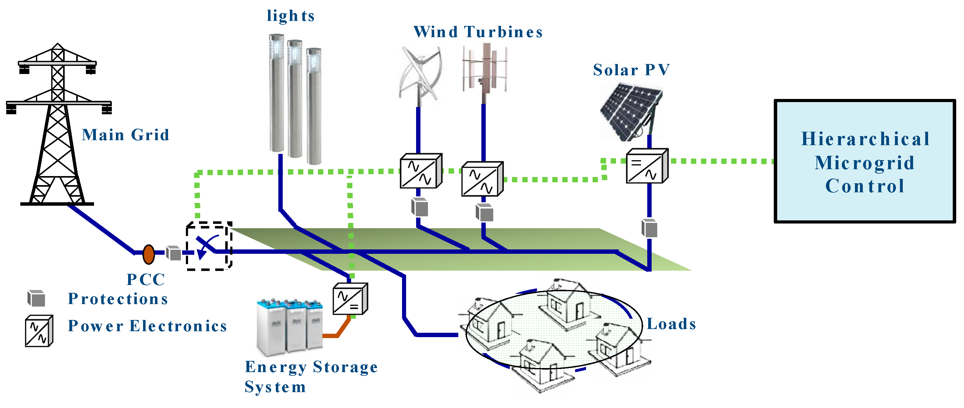
In a microgrid, multiple distributed generators (DG) and loads are connected to a point of common coupling (PCC) as shown in Figure 1. The loads connected to the microgrid may be supplied by the DGs or by a direct connection to the main grid. In addition, multiple energy storage units may be connected to the microgrid to increase the power availability and system reliability [2].

A microgrid requires the use of power electronics devices to perform the energy conversion from one voltage level to another. For example, for an AC microgrid, the energy storage system (ESS) requires the use of a bidirectional AC–DC converter that regulates the charge or discharge process depending on the available energy. Wind turbine generators require the use of AC–AC converters to transform the amplitude and frequency to standardized voltage levels in the microgrid. Solar photovoltaic (PV) generators require the use of a DC–AC converter to inject the maximum available energy to the microgrid. Loads such as residential homes and streetlights are connected to the microgrid’s common bus. The common bus may be connected to the main grid or disconnected to be operating in islanded mode. Each of the interconnections mentioned above are managed by one or more controllers to optimize the energy generation, guarantee adequate power quality, and to improve stability and robustness in the microgrid.

Optimal controllers for microgrids are aimed to achieve the best performance and/or stability margins by applying numerical optimization methods to the open-loop model. Some relevant works related to the optimal control applied to Voltage-Current (V-I) control level may be found in [3,4,5,6,7,8,9,10,11,12]. Most of these works use proportional–integral (PI) or proportional–resonant (PR) controllers with linear quadratic (LQ) control to compute an optimal state-feedback matrix that minimizes certain cost functions. Optimal LQ strategies for primary control are more difficult to implement since this kind of controllers require an open-loop model to apply numerical optimization methods.

In [13], the authors presented a small signal stability analysis for a single-phase droop controlled inverter connected to a stiff AC source. In this analysis, a resistive-inductive load is connected between the inverter and the stiff AC source. The expressions to compute the active power P and reactive power Q expressions are presented as follows:

$$\mathrm{P}=-\frac{1}{{\mathrm{R}}^2{+\mathrm{X}}^2}\left({\mathrm{RE}}^2-\mathrm{REV}\cos \mathsf{\delta }+\mathrm{XEV}\sin \mathsf{\delta }\right)$$

(1)

$$\mathrm{Q}=-\frac{1}{{\mathrm{R}}^2{+\mathrm{X}}^2}\left({\mathrm{XE}}^2-\mathrm{XEV}\cos \mathsf{\delta }-\mathrm{REV}\sin \mathsf{\delta }\right)$$

(2)

where R and X are the real and imaginary components of the line impedance. E and V are the voltage amplitude of the inverter and stiff AC source, respectively. Finally, the phase difference between both generators is defined by $\mathsf{\delta }$. For small disturbances, the above equations can be linearized as follows:

$$\mathsf{\Delta }\mathrm{P}=\frac{\partial \mathrm{P}}{\partial \mathrm{E}}\mathsf{\Delta }\mathrm{E}+\frac{\partial \mathrm{P}}{\partial \mathsf{\delta }}\mathsf{\Delta }\mathsf{\delta }$$

(3)

$$\mathsf{\Delta }\mathrm{Q}=\frac{\partial \mathrm{Q}}{\partial \mathrm{E}}\mathsf{\Delta }\mathrm{E}+\frac{\partial \mathrm{Q}}{\partial \mathsf{\delta }}\mathsf{\Delta }\mathsf{\delta }.$$

(4)

The linearized expressions for P, Q, $\mathsf{\omega }$, and E are given by

$${\mathsf{\Delta }\mathrm{P}=\mathrm{k}}_{\mathrm{pe}}{\mathsf{\Delta }\mathrm{E}+\mathrm{k}}_{\mathrm{pd}}\mathsf{\Delta }\mathsf{\delta }$$

(5)

$${\mathsf{\Delta }\mathrm{Q}=\mathrm{k}}_{\mathrm{qe}}{\mathsf{\Delta }\mathrm{E}+\mathrm{k}}_{\mathrm{qd}}\mathsf{\Delta }\mathsf{\delta }$$

(6)

$$\mathsf{\Delta }\mathsf{\omega }=-\mathrm{m}\mathsf{\Delta }\mathrm{P}$$

(7)

$$\mathsf{\Delta }\mathrm{E}=-\mathrm{n}\mathsf{\Delta }\mathrm{Q}$$

(8)

where ${\mathrm{k}}_{\mathrm{pe}},{\mathrm{k}}_{\mathrm{pd}},{\mathrm{k}}_{\mathrm{qe}},$ and ${\mathrm{k}}_{\mathrm{qd}}$ are the constants resulting from evaluating the linearization function on the operating point $\left({\mathsf{\delta }}_{\mathrm{e}}{,\mathrm{E}}_{\mathrm{e}},{\mathrm{V}}_{\mathrm{e}}\right)$ [13]. Equations (7) and (8) represent the droop control equations, where $\mathsf{\Delta }\mathsf{\omega }\left(\mathrm{s}\right)=\mathrm{s}\mathsf{\delta }\left(\mathrm{s}\right)$ is the frequency deviation around the operating point ${\mathsf{\omega }}_{\mathrm{e}}$. Using a low-pass filter with the cut-off frequency ${\mathsf{\omega }}_{\mathrm{f}}$ and merging Equation (5) into (8), the following system is defined:

$$\mathsf{\Delta }\mathsf{\delta }\left(\mathrm{s}\right)=-\frac{{\mathrm{m}\mathsf{\omega }}_{\mathrm{f}}}{\mathrm{s}\left({\mathrm{s}+\mathsf{\omega }}_{\mathrm{f}}\right)}\left({\mathrm{k}}_{\mathrm{pe}}\mathsf{\Delta }\mathrm{E}\left(\mathrm{s}\right){+\mathrm{k}}_{\mathrm{pd}}\mathsf{\Delta }\mathsf{\delta }\left(\mathrm{s}\right)\right)$$

(9)

$$\mathsf{\Delta }\mathrm{E}\left(\mathrm{s}\right)=-\frac{{\mathrm{n}\mathsf{\omega }}_{\mathrm{f}}}{{\mathrm{s}+\mathsf{\omega }}_{\mathrm{f}}}\left({\mathrm{k}}_{\mathrm{qe}}\mathsf{\Delta }\mathrm{E}\left(\mathrm{s}\right){+\mathrm{k}}_{\mathrm{qd}}\mathsf{\Delta }\mathsf{\delta }\left(\mathrm{s}\right)\right).$$

(10)

The analysis performed in [13] is used to determine the stability of a droop-controlled inverter connected to a stiff AC source. This is done by analyzing the resulting eigenvalues of the system generated by Equations (9) and (10). It can also be noticed that, for suitable values of m and n, the inverter frequency and voltage amplitude will converge to zero deviation from the operating point.

Following this work, Coelho et al. presented a similar small-signal stability analysis for the two parallel connected inverters sharing power between them [14]. In this work, a state-space representation of the entire linearized microgrid was developed in the dq frame. The entire system is described in (11):

$$\mathsf{\Delta }\stackrel{·}{\mathrm{x}}=\mathrm{A}·\mathsf{\Delta }\mathrm{x}$$

(11)

with $\mathsf{\Delta }\mathrm{x}={\left[\begin{array}{ccc}\begin{array}{cc}{\mathsf{\Delta }\mathsf{\omega }}_1& {\mathsf{\Delta }\mathrm{E}}_{\mathrm{d}1}\end{array}& \begin{array}{cc}{\mathsf{\Delta }\mathrm{E}}_{\mathrm{q}1}& {\mathsf{\Delta }\mathsf{\omega }}_2\end{array}& \begin{array}{cc}{\mathsf{\Delta }\mathrm{E}}_{\mathrm{d}2}& {\mathsf{\Delta }\mathrm{E}}_{\mathrm{q}2}\end{array}\end{array}\right]}^{\mathrm{T}}$. States ${\mathsf{\Delta }\mathrm{E}}_{\mathrm{di}}$ and ${\mathsf{\Delta }\mathrm{E}}_{\mathrm{qi}}$ are the in-phase and quadrature nominal voltage in the dq frame for the i-th inverter and ${\mathsf{\Delta }\mathsf{\omega }}_{\mathrm{i}}$ is the frequency of each inverter. The state matrix ${\mathrm{A}=\mathrm{M}}_{\mathrm{s}}{+\mathrm{C}}_{\mathrm{s}}\left({\mathrm{I}}_{\mathrm{s}}{+\mathrm{E}}_{\mathrm{s}}{\mathrm{Y}}_{\mathrm{s}}\right){\mathrm{K}}_{\mathrm{s}}$ is composed of matrices that are dependent of the droop coefficients, the nominal voltages, and the nominal currents vector. Refer to [14] for a detailed definition of these matrices. Knowing the value of matrix $\mathrm{A}$, the eigenvalues may be calculated to determine the stability and transient response of the entire system. The work by Coelho et al. provided an effective method for analyzing stability in microgrids using the droop method as a primary control strategy. However, this analysis does not consider the effects of the V-I control loop and does not allow to separate the droop controller and the system.

In [15], a complete microgrid was modeled using small-signal analysis. The V-I and power sharing control levels where integrated to analyze their influence on microgrid stability. The complete system was modeled in three different parts: inverter model, network model, and load model. In the inverter model, the V-I and primary droop control were considered together with the inductor–capacitor–inductor (LCL) output filter dynamics. In the network model, a network with m nodes and n resistive-inductive lines was considered. In the load model, a resistive-inductive load was modeled. Each of these models was written in such a way that the complete microgrid model may integrate them depending on the number of generators, network interconnections, and loads.

The complete model was analyzed using the root locus method. It was discovered that there were three different relevant clusters in the microgrid’s eigenvalues placement. This approach shows relevant information regarding microgrid stability using small signal analysis. However, the complete microgrid model relies entirely on the control topology and control constants. Generally, a dynamic system is modeled in such a way that the designer may easily couple it with a control strategy. However, in this approach, the control parameters are embedded into the microgrid model and changing them directly affects the analysis. Moreover, no formal stability analysis can be performed from an open-loop perspective because the microgrid model can only be developed considering the closed loop system.

Another important work regarding microgrid stability with droop controllers is presented in [16]. The author divides microgrid stability in three main categories: small signal stability, transient stability, and voltage stability. The small signal stability is mainly affected by the V-I and primary feedback controllers, where the control parameters affect system transient response and pole allocation. The use of feedback controllers with decentralized control methods such as droop control creates most of the small signal stability issues in islanded microgrids [16]. This stability can be improved by using robust and optimal control techniques, supplementary control loops, coordinated control, and stabilizers such as flywheels. Transient stability is mainly affected in islanded mode, were frequency and voltage amplitude may be affected without a connection to a stiff grid. Transient stability is analyzed by using Lyapunov function techniques and nonlinear system analysis [17]. In addition, transient stability can be addressed by using energy storage and load shedding methods which allow to sustain the entire system when a sudden power loss is detected. Finally, voltage stability may be caused by irregular behavior in reactive load sharing or the connection of induction motors. Voltage stability can be addressed by injecting reactive power into the microgrid and compensate the sudden voltage droop.

Another approach for stability analysis in droop controllers is performed in [18], where a dynamic phasor modeling (DPM) of the primary droop control of a microgrid was developed. The DPM allows to introduce additional terms on the imaginary axis to the mathematical model. This consideration makes the DPM of the inverter circuit more accurate than the conventional small signal analysis shown in [14]. A new active and reactive power model was developed, and its accuracy was compared to a complete order model and a small signal model. Results show adequate modeling in transient response and eigenvalue location. In addition, a virtual-frame droop control was tested with this model with more accurate results than in previous work. However, this model does not consider the V-I control loop and makes it difficult to analyze the coupling between the real and imaginary components of power, current, and impedances. This modeling could result more effective when analyzing transient responses in a complete microgrid.

In this document, a model for inverter-based grid-connected and islanded microgrids in a synchronous reference frame is presented. Both models were tested and validated in an experimental setup to demonstrate their accuracy in describing microgrid dynamics. Most of the approaches found in the literature developed the microgrid model based on the controller dynamics, which does not allow to perform an open-loop analysis such as singular value diagrams or obtaining stability margins. The aim of the proposed models is to allow designers to perform robustness and stability analysis techniques that require an open-loop model to be performed. In addition, the proposed models are able to be used to develop controllers that are based on numerical optimization methods such as linear quadratic controllers, Kalman filters, ${\mathrm{H}}_{\infty }$-based controllers, model-predictive controllers, and others. The presented models are small-signal realizations that consider parameters such as frequency around the operating equilibrium point. Although the proposed models are developed for a microgrid based on inverter generators connected to a single point of common coupling (PCC), the methodology used to develop them may be used to expand the case study to more complex microgrids.

Three application scenarios are presented: non-controlled model, Linear-Quadratic Integrator (LQI) power control, and Power-Voltage (PQ/Vdq) droop–boost controller. Both controllers allow to perform stability and performance analysis methods which, unlike approaches found in the literature, can provide a wider perspective of the microgrid in islanded and grid-connected modes. Furthermore, the controlled open-loop model can be used to analyze the microgrid frequency response under disturbances in the process and noise in the sensors. The linear nature of the proposed controllers allows to compute modern controllers that rely on a precise model to obtain a controller that optimizes certain control objectives.

The following sections are divided as follows: Section 2 presents the mathematical development of the proposed models; and Section 3 presents the validation of the proposed model under three different scenarios. Finally, the discussion of results is presented in Section 4.

2. Microgrid Model

The proposed model for this research is obtained in two stages. First, the model of each inverter connected to the main grid is used to describe dynamics in grid-connected mode. This model is also used to develop the proposed control strategy. Then, the models of all inverters are integrated in a single state-space model to describe the microgrid dynamics in islanded mode.

2.1. Model of a Single Inverter Connected to the Main Grid

The circuit used to develop the proposed model in grid-connected mode is shown in Figure 2. The output of a three-phase inverter $\mathrm{E}$ is driven by a Pulsed-Width Modulated (PWM) signal, which is filtered using an inductor–capacitor–inductor (LCL) output filter. The inverter is connected to a stiff voltage source $\mathrm{V}$ that represents the main grid. Input inductor current, capacitor voltage, and output current are denoted by ${\mathrm{I}}_{\mathrm{l}}$, ${\mathrm{V}}_{\mathrm{c}}$, and ${\mathrm{I}}_{\mathrm{o}}$, respectively.

The state-space model of this circuit for each phase in the ABC frame is given by

$$\left[\begin{array}{c}{\stackrel{·}{\mathrm{V}}}_{\mathrm{c}}\\ {\stackrel{·}{\mathrm{I}}}_{\mathrm{l}}\\ {\stackrel{·}{\mathrm{I}}}_{\mathrm{o}}\end{array}\right]\left[\begin{array}{ccc}0& \raisebox{1ex}{$1$}\!\left/ \!\raisebox{-1ex}{$\mathrm{C}$}\right.& -\raisebox{1ex}{$1$}\!\left/ \!\raisebox{-1ex}{$\mathrm{C}$}\right.\\ -\raisebox{1ex}{$1$}\!\left/ \!\raisebox{-1ex}{${\mathrm{L}}_{\mathrm{i}}$}\right.& 0& 0\\ \raisebox{1ex}{$1$}\!\left/ \!\raisebox{-1ex}{${\mathrm{L}}_{\mathrm{o}}$}\right.& 0& 0\end{array}\right]\left[\begin{array}{c}{\mathrm{V}}_{\mathrm{c}}\\ {\mathrm{I}}_{\mathrm{l}}\\ {\mathrm{I}}_{\mathrm{o}}\end{array}\right]+\left[\begin{array}{c}0\\ \raisebox{1ex}{$1$}\!\left/ \!\raisebox{-1ex}{${\mathrm{L}}_{\mathrm{i}}$}\right.\\ 0\end{array}\right]\mathrm{E}+\left[\begin{array}{c}0\\ 0\\ -\raisebox{1ex}{$1$}\!\left/ \!\raisebox{-1ex}{${\mathrm{L}}_{\mathrm{o}}$}\right.\end{array}\right]{\mathrm{V}}_{\mathrm{g}}.$$

(12)

It is important to note that, in order to simplify the mathematical procedure, this model does not consider non-linear phenomenon such as the switching behavior in the insulated-gate bipolar transistors (IGBT), the voltage saturation in the DC bus, nor the unbalances caused by the deviation in its components. In addition, no phenomenon related to AC–AC conversion using power transformers is considered. The state-space model (13) is obtained using the dq transformation. The state-space model transformation to the dq frame is based on the Clarke transformation and the complete mathematical development may be found in [19]. The dq transformation is performed by assuming a constant angular frequency ${\mathsf{\omega }}_{\mathrm{c}}$, which corresponds to the nominal angular frequency of the main grid:

$$\stackrel{·}{\mathrm{x}}={\mathrm{A}}_{\mathrm{dq}}\mathrm{x}+{\mathrm{B}}_{1\mathrm{dq}}{\mathrm{E}}_{\mathrm{dq}}+{\mathrm{B}}_{2\mathrm{dq}}+{\mathrm{V}}_{\mathrm{gdq}}$$

(13)

where ${\mathrm{E}}_{\mathrm{dq}}={\left[\begin{array}{cc}{\mathrm{E}}_{\mathrm{d}}& {\mathrm{E}}_{\mathrm{q}}\end{array}\right]}^{\mathrm{T}}$, ${\mathrm{V}}_{\mathrm{gdq}}={\left[\begin{array}{cc}{\mathrm{V}}_{\mathrm{gd}}& {\mathrm{V}}_{\mathrm{gq}}\end{array}\right]}^{\mathrm{T}}$, and:

$$\mathrm{x}=\left[\begin{array}{c}\begin{array}{c}{\mathrm{V}}_{\mathrm{cd}}\\ {\mathrm{V}}_{\mathrm{cq}}\end{array}\\ \begin{array}{c}{\mathrm{I}}_{\mathrm{ld}}\\ {\mathrm{I}}_{\mathrm{lq}}\end{array}\\ \begin{array}{c}{\mathrm{I}}_{\mathrm{od}}\\ {\mathrm{I}}_{\mathrm{oq}}\end{array}\end{array}\right];{\mathrm{A}}_{\mathrm{dq}}=\left[\begin{array}{cccccc}0& {\mathsf{\omega }}_{\mathrm{c}}& 1/\mathrm{C}& 0& -1/C& 0\\ {-\mathsf{\omega }}_{\mathrm{c}}& 0& 0& 1/\mathrm{C}& 0& -1/C\\ -1/{\mathrm{L}}_{\mathrm{i}}& 0& 0& {\mathsf{\omega }}_{\mathrm{c}}& 0& 0\\ 0& -1/{\mathrm{L}}_{\mathrm{i}}& {-\mathsf{\omega }}_{\mathrm{c}}& 0& 0& 0\\ 1/{\mathrm{L}}_{\mathrm{o}}& 0& 0& 0& 0& {\mathsf{\omega }}_{\mathrm{c}}\\ 0& 1/{\mathrm{L}}_{\mathrm{o}}& 0& 0& {-\mathsf{\omega }}_{\mathrm{c}}& 0\end{array}\right];{\mathrm{B}}_{1\mathrm{dq}}=\left[\begin{array}{cc}0& 0\\ 0& 0\\ {1/\mathrm{L}}_{\mathrm{i}}& 0\\ 0& {1/\mathrm{L}}_{\mathrm{i}}\\ 0& 0\\ 0& 0\end{array}\right];{\mathrm{B}}_{2\mathrm{dq}}=\left[\begin{array}{cc}0& 0\\ 0& 0\\ 0& 0\\ 0& 0\\ {-1/\mathrm{L}}_{\mathrm{o}}& 0\\ 0& {-1/\mathrm{L}}_{\mathrm{o}}\end{array}\right].$$

(14)

The active and reactive power injected to ${\mathrm{V}}_{\mathrm{gdq}}$ are defined by

$$\mathrm{P}=\frac{3}{2}\left({\mathrm{V}}_{\mathrm{gd}}{\mathrm{I}}_{\mathrm{od}}{+\mathrm{V}}_{\mathrm{gq}}{\mathrm{I}}_{\mathrm{oq}}\right)$$

(15)

$$\mathrm{Q}=\frac{3}{2}\left({\mathrm{V}}_{\mathrm{gq}}{\mathrm{I}}_{\mathrm{d}}{-\mathrm{V}}_{\mathrm{gd}}{\mathrm{I}}_{\mathrm{oq}}\right)$$

(16)

The dq frame is synchronized with the main grid by using a Phase-Locked Loop (PLL). Thus, ${\mathrm{V}}_{\mathrm{gd}}$ represents the nominal voltage peak amplitude of the main grid, ${\overline{\mathrm{V}}}_{\mathrm{gd}}$ and ${\overline{\mathrm{V}}}_{\mathrm{gq}}=0$ [19]. This is because the PLL increases the angular frequency ω until the q component of the three-phase signal becomes zero. Thus, the output of the state-space model is used to represent the active and reactive power received by ${\mathrm{V}}_{\mathrm{gdq}}$ as follows:

$$\mathrm{Y}=\left[\begin{array}{c}\mathrm{P}\\ \mathrm{Q}\end{array}\right]=\frac{3}{2}\left[\begin{array}{cc}{\overline{\mathrm{V}}}_{\mathrm{gd}}& 0\\ 0& -{\overline{\mathrm{V}}}_{\mathrm{gd}}\end{array}\right]\left[\begin{array}{c}{\mathrm{I}}_{\mathrm{od}}\\ {\mathrm{I}}_{\mathrm{oq}}\end{array}\right].$$

(17)

It is important to remark that the system in (13) must be discretized in order to implement it in a physical experiment using data acquisition devices and PWM control signals. To discretize it, the state must be augmented using a delay transfer function to account for the delay induced by the PWM output signal [20,21]. The resulting system is given by

$$\stackrel{{\mathrm{X}}_{\mathrm{T}}\left[\mathrm{k}+1\right]}{\overbrace{\left[\begin{array}{c}\mathrm{X}\left[\mathrm{k}+1\right]\\ {\mathrm{E}}_{-1}\left[\mathrm{k}+1\right]\end{array}\right]}}=\stackrel{{\mathrm{A}}_{\mathrm{T}}}{\overbrace{\left[\begin{array}{cc}{\overline{\mathrm{A}}}_{\mathrm{dq}}& {\overline{\mathrm{B}}}_{1\mathrm{dq}}\\ 0_{2\times 6}& 0_{2\times 2}\end{array}\right]}}\stackrel{{\mathrm{X}}_{\mathrm{T}}\left[\mathrm{k}\right]}{\overbrace{\left[\begin{array}{c}\mathrm{X}\left[\mathrm{k}\right]\\ {\mathrm{E}}_{-1}\left[\mathrm{k}\right]\end{array}\right]}}\stackrel{{\mathrm{B}}_{1\mathrm{T}}}{\overbrace{\left[\begin{array}{c}{0}_{6\times 2}\\ {\mathrm{I}}_{2\times 2}\end{array}\right]}}{\mathrm{E}}_{\mathrm{dq}}\left[\mathrm{k}\right]+\stackrel{{\mathrm{B}}_{2\mathrm{T}}}{\overbrace{\left[\begin{array}{c}{\mathrm{B}}_{2\mathrm{dq}}\\ 0_{2\times 2}\end{array}\right]}}{\mathrm{V}}_{\mathrm{gdq}}\left[\mathrm{k}\right]$$

(18)

where ${\overline{\mathrm{A}}}_{\mathrm{dq}}$ and ${\overline{\mathrm{B}}}_{1\mathrm{dq}}$ are the discrete-time state and input matrices. The auxiliary variable ${\mathrm{E}}_{-1}$ represents the delayed input and the discrete-time state vector in the dq frame is $\mathrm{X}\left[\mathrm{k}\right]={\left[\begin{array}{cccccc}{\mathrm{V}}_{\mathrm{cd}}& {\mathrm{V}}_{\mathrm{cq}}& {\mathrm{I}}_{\mathrm{ld}}& {\mathrm{I}}_{\mathrm{lq}}& {\mathrm{I}}_{\mathrm{od}}& {\mathrm{I}}_{\mathrm{oq}}\end{array}\right]}^{\mathrm{T}}$.

2.2. Model of the Microgrid in Islanded Mode

The islanded microgrid model was used to assess the stability and robustness considering the interaction of multiple inverters connected in islanded mode to a single PCC. For the grid-connected mode, the state-space model (13) must be used for each generator individually. The circuit considered for the islanded microgrid model is shown in Figure 3. This circuit only considers interactions between inverter-based generators and the main grid from a single PCC. However, the methods proposed in this section may be used to integrate the proposed model into more complex microgrids. The integration of the proposed model with a microgrid with synchronous generators is out of the scope of this work.

Although, many types of loads may exist in microgrids, so the load is selected to be a resistive-inductive ($\mathrm{RL}$) circuit because it allows to analyze the behavior of the active and reactive power. To obtain the complete microgrid model, the model for one phase of each inverter using (12) must be computed. Then, ${\mathrm{V}}_{\mathrm{g}}$ must be defined in terms of the output currents and load components as follows:

$${\mathrm{V}}_{\mathrm{g}}=\mathrm{L}{\stackrel{·}{\mathrm{I}}}_{\mathrm{ot}}+\mathrm{R}{\mathrm{I}}_{\mathrm{ot}}$$

(19)

where ${\mathrm{I}}_{\mathrm{ot}}={{\displaystyle \sum }}_{\mathrm{j}=1}^{\mathrm{n}}{\mathrm{I}}_{\mathrm{oj}}$ with $\mathrm{n}$ representing the number of generators. Equation (19) can be reformulated to describe the resistive-capacitive behavior in order to analyze loads such as LED lighting or AC–DC converters. Nonlinear loads with harmonic currents can be modeled as a disturbance in the complete model with a known bandwidth and frequency behavior. A complete microgrid model is obtained by substituting ${\mathrm{V}}_{\mathrm{g}}$ from (19) into the model of each inverter (12) and combining all the models. For example, for two generators with a common RL load, the microgrid model in islanded mode for one phase is given by (20):

$$\left[\begin{array}{c}{\dot{\mathrm{V}}}_{\mathrm{c}1}\\ {\dot{\mathrm{I}}}_{\mathrm{l}1}\\ {\dot{\mathrm{I}}}_{\mathrm{o}1}\\ {\dot{\mathrm{V}}}_{\mathrm{c}2}\\ {\dot{\mathrm{I}}}_{\mathrm{l}2}\\ {\dot{\mathrm{I}}}_{\mathrm{o}2}\end{array}\right]=\left[\begin{array}{cccccc}0& {1/\mathrm{C}}_1& {-1/\mathrm{C}}_1& 0& 0& 0\\ {-1/\mathrm{L}}_{\mathrm{i}1}& 0& 0& 0& 0& 0\\ {\mathrm{L}}_{\mathrm{t}2}{/\mathrm{L}}_{\mathrm{dt}}& 0& \left({\mathrm{RL}-\mathrm{RL}}_{\mathrm{t}2}\right){/\mathrm{L}}_{\mathrm{dt}}& {-\mathrm{L}/\mathrm{L}}_{\mathrm{dt}}& 0& \left({\mathrm{RL}-\mathrm{RL}}_{\mathrm{t}2}\right){/\mathrm{L}}_{\mathrm{dt}}\\ 0& 0& 0& 0& {1/\mathrm{C}}_2& {-1/\mathrm{C}}_2\\ 0& 0& 0& {-1/\mathrm{L}}_{\mathrm{i}2}& 0& 0\\ {-\mathrm{L}/\mathrm{L}}_{\mathrm{dt}}& 0& \left({\mathrm{RL}-\mathrm{RL}}_{\mathrm{t}1}\right){/\mathrm{L}}_{\mathrm{dt}}& {\mathrm{L}}_{\mathrm{t}1}{/\mathrm{L}}_{\mathrm{t}}& 0& \left({\mathrm{RL}-\mathrm{RL}}_{\mathrm{t}1}\right){/\mathrm{L}}_{\mathrm{dt}}\end{array}\right]\left[\begin{array}{c}{\mathrm{V}}_{\mathrm{c}1}\\ {\mathrm{I}}_{\mathrm{l}1}\\ {\mathrm{I}}_{\mathrm{o}1}\\ \begin{array}{c}{\mathrm{V}}_{\mathrm{c}2}\\ {\mathrm{I}}_{\mathrm{l}2}\\ {\mathrm{I}}_{\mathrm{o}2}\end{array}\end{array}\right]+\left[\begin{array}{cc}0& 0\\ {1/\mathrm{L}}_{\mathrm{i}1}& 0\\ 0& 0\\ 0& 0\\ 0& {1/\mathrm{L}}_{\mathrm{i}2}\\ 0& 0\end{array}\right]\left[\begin{array}{c}{\mathrm{E}}_1\\ {\mathrm{E}}_2\end{array}\right]$$

(20)

where ${\mathrm{L}}_{\mathrm{dt}}=\mathrm{L}\left({\mathrm{L}}_{\mathrm{o}1}{+\mathrm{L}}_{\mathrm{o}2}\right){+\mathrm{L}}_{\mathrm{o}1}{\mathrm{L}}_{\mathrm{o}2}$, ${\mathrm{L}}_{\mathrm{t}1}{=\mathrm{L}+\mathrm{L}}_{\mathrm{o}1}$, and ${\mathrm{L}}_{\mathrm{t}2}{=\mathrm{L}+\mathrm{L}}_{\mathrm{o}2}$. For $\mathrm{n}$ inverters, replacing ${\mathrm{V}}_{\mathrm{g}}$ from (19) into each generator model (12) yields to a linear system with the differential equations for the output currents as shown in (21). Combining the solution of (21) with the model of each inverter (12), the complete microgrid model (22) for $\mathrm{n}$ inverters is obtained. The model in (22) is for each phase. However, it must be transformed to the dq frame using as in [19]:

$$\left[\begin{array}{c}{\dot{\mathrm{I}}}_{\mathrm{o}1}\\ {\dot{\mathrm{I}}}_{\mathrm{o}2}\\ ⋮\\ {\dot{\mathrm{I}}}_{\mathrm{on}-1}\\ {\dot{\mathrm{I}}}_{\mathrm{on}}\end{array}\right]=\left[\begin{array}{ccccc}\left({\mathrm{L}}_{\mathrm{o}1}+\mathrm{L}\right)& \mathrm{L}& \cdots & \mathrm{L}& \mathrm{L}\\ \mathrm{L}& \left({\mathrm{L}}_{\mathrm{o}2}+\mathrm{L}\right)& \cdots & \mathrm{L}& \mathrm{L}\\ ⋮& ⋮& \ddots & ⋮& ⋮\\ \mathrm{L}& \mathrm{L}& \dots & \left({\mathrm{L}}_{\mathrm{on}-1}+\mathrm{L}\right)& \mathrm{L}\\ \mathrm{L}& \mathrm{L}& \cdots & \mathrm{L}& \left({\mathrm{L}}_{\mathrm{on}}+\mathrm{L}\right)\end{array}\right]\left[\begin{array}{c}{\mathrm{V}}_{\mathrm{c}1}{-\mathrm{RI}}_{\mathrm{t}}\\ {\mathrm{V}}_{\mathrm{c}2}{-\mathrm{RI}}_{\mathrm{t}}\\ ⋮\\ {\mathrm{V}}_{\mathrm{cn}-1}{-\mathrm{RI}}_{\mathrm{t}}\\ {\mathrm{V}}_{\mathrm{cn}}{-\mathrm{RI}}_{\mathrm{t}}\end{array}\right]=\left[\begin{array}{ccc}{\mathsf{\varphi }}_{11}& \cdots & {\mathsf{\varphi }}_{1\mathrm{n}}\\ ⋮& \ddots & ⋮\\ {\mathsf{\varphi }}_{\mathrm{n}1}& \cdots & {\mathsf{\varphi }}_{\mathrm{nn}}\end{array}\right]\left[\begin{array}{c}{\mathrm{V}}_{\mathrm{c}1}\\ {\mathrm{I}}_{\mathrm{l}1}\\ {\mathrm{I}}_{\mathrm{o}1}\\ ⋮\\ \begin{array}{c}{\mathrm{V}}_{\mathrm{cn}}\\ {\mathrm{I}}_{\ln }\\ {\mathrm{I}}_{\mathrm{on}}\end{array}\end{array}\right]$$

(21)

$$\left[\begin{array}{c}{\dot{\mathrm{V}}}_{\mathrm{c}1}\\ {\dot{\mathrm{I}}}_{\mathrm{l}1}\\ {\dot{\mathrm{I}}}_{\mathrm{o}1}\\ ⋮\\ \begin{array}{c}{\dot{\mathrm{V}}}_{\mathrm{cn}}\\ {\dot{\mathrm{I}}}_{\ln }\\ {\dot{\mathrm{I}}}_{\mathrm{on}}\end{array}\end{array}\right]=\stackrel{{\mathrm{A}}_{\mathsf{\mu }\mathrm{G}}}{\overbrace{\left[\begin{array}{ccccc}{\tilde{\mathrm{A}}}_1& 0_{2\times 3}& \cdots & \cdots & 0_{2\times 3}\\ {\mathsf{\varphi }}_{11}& {\mathsf{\varphi }}_{12}& \cdots & {\mathsf{\varphi }}_{1\mathrm{n}-1}& {\mathsf{\varphi }}_{1\mathrm{n}}\\ 0_{2\times 3}& \cdots & {\tilde{\mathrm{A}}}_2& \cdots & 0_{2\times 3}\\ {\mathsf{\varphi }}_{21}& {\mathsf{\varphi }}_{22}& \cdots & {\mathsf{\varphi }}_{2\mathrm{n}-1}& {\mathsf{\varphi }}_{2\mathrm{n}}\\ ⋮& ⋮& ⋮& ⋮& ⋮\\ 0_{2\times 3}& \dots & \dots & 0_{2\times 3}& {\tilde{\mathrm{A}}}_{\mathrm{n}}\\ {\mathsf{\varphi }}_{\mathrm{n}1}& {\mathsf{\varphi }}_{\mathrm{n}2}& \dots & {\mathsf{\varphi }}_{\mathrm{nn}-1}& {\mathsf{\varphi }}_{\mathrm{nn}}\end{array}\right]}}\stackrel{{\mathrm{X}}_{\mathsf{\mu }\mathrm{G}}}{\overbrace{\left[\begin{array}{c}{\mathrm{V}}_{\mathrm{c}1}\\ {\mathrm{I}}_{\mathrm{l}1}\\ {\mathrm{I}}_{\mathrm{o}1}\\ ⋮\\ \begin{array}{c}{\mathrm{V}}_{\mathrm{cn}}\\ {\mathrm{I}}_{\ln }\\ {\mathrm{I}}_{\mathrm{on}}\end{array}\end{array}\right]}}+\stackrel{{\mathrm{B}}_{\mathsf{\mu }\mathrm{G}}}{\overbrace{\left[\begin{array}{ccc}{\mathrm{B}}_1& \dots & 0_{3\times 1}\\ ⋮& \ddots & ⋮\\ 0_{3\times 1}& \dots & {\mathrm{B}}_{\mathrm{n}}\end{array}\right]}}\left[\begin{array}{c}{\mathrm{E}}_1\\ ⋮\\ {\mathrm{E}}_{\mathrm{n}}\end{array}\right]$$

(22)

where:

$${\tilde{\mathrm{A}}}_{\mathrm{j}}=\left[\begin{array}{ccc}0& {1/\mathrm{C}}_{\mathrm{j}}& {-1/\mathrm{C}}_{\mathrm{j}}\\ {-1/\mathrm{L}}_{\mathrm{j}}& 0& 0\end{array}\right],{\mathrm{B}}_{\mathrm{j}}={\left[\begin{array}{ccc}0& 1/{\mathrm{L}}_{\mathrm{ij}}& 0\end{array}\right]}^{\mathrm{T}}$$

(23)

with $1\le \mathrm{j}\le \mathrm{n}$. Elements ${\mathsf{\varphi }}_{\mathrm{jk}}$ represent the coefficients of each state variable properly arranged from the solution of (21).

3. Validation of the Proposed Models and Application Scenarios

The proposed models were validated in three scenarios:

• Open-loop model validation;
• Grid-connected LQI power controller;
• Islanded PQ/Vdq LQI-based droop controller.

The open-loop model validation is used to assess the similarity between the mathematical model and the physical model. The grid connected LQI power controller is used to demonstrate the applicability of the model for a single inverter. Finally, the islanded PQ/Vdq LQI-based droop controller is used to assess the stability and performance of an entire microgrid in islanded mode.

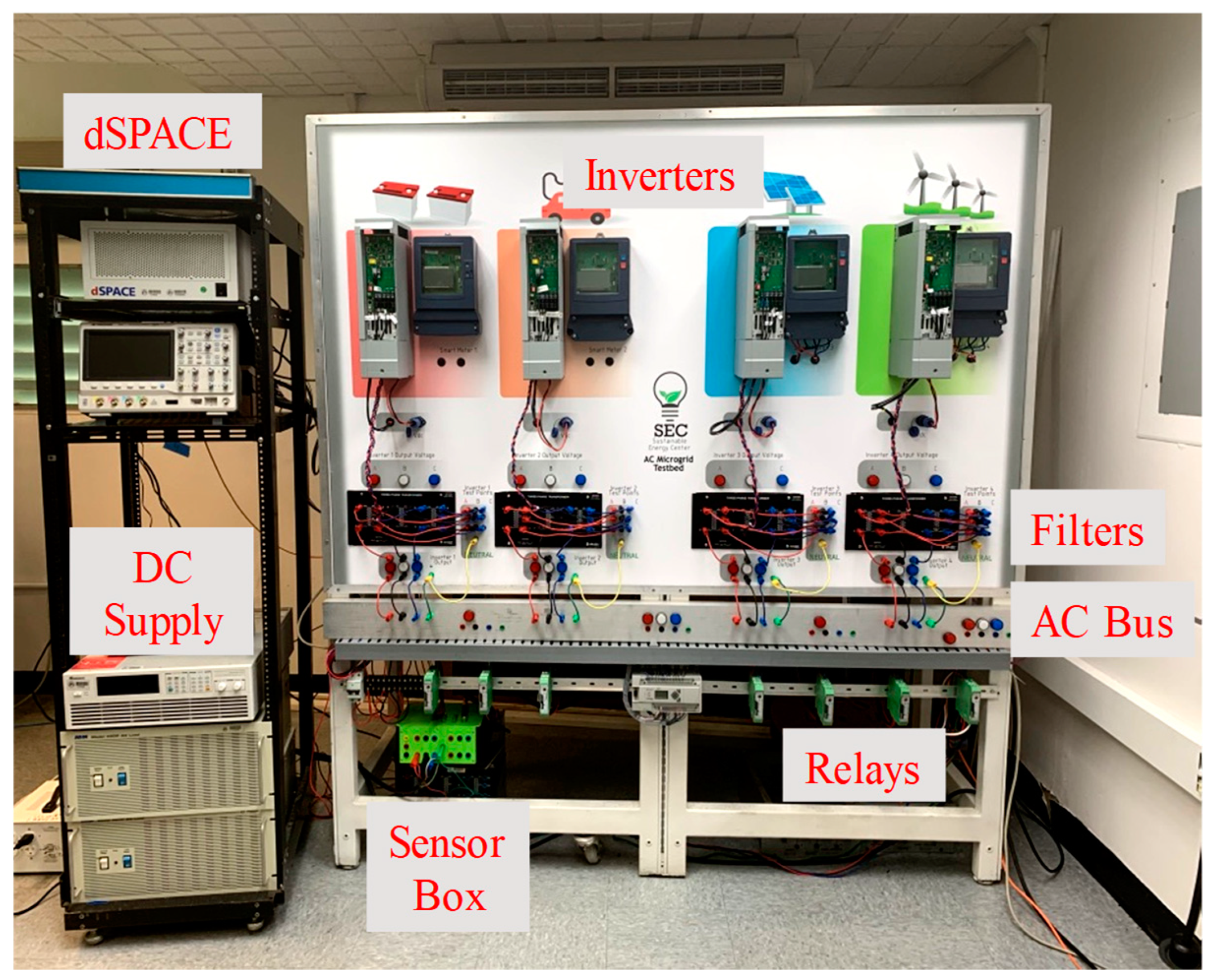
For safety reasons, the open-loop model of the grid-connected and islanded microgrid were not validated in a real experiment. Instead, these models were validated using an OPAL-RT OP5700 Real-time simulator. The closed-loop models were validated using the setup shown in Figure 4. This setup uses four Danfoss 2.2 kVA inverters with LCL filters and four sensor boxes with voltage and current sensors from LEM International. These four inverters may be dynamically connected to the AC bus. The AC bus may also be dynamically connected or disconnected from the main grid using solid-state relays handled with a programmable logic controller (PLC). To implement the control algorithms, a dSPACE 1006 simulator was used to read the signals from the sensor boxes and send the 10 kHz PWM pulses via optical fiber.

For each scenario, the time responses of each inverter were compared with the mathematical model. In addition, the mathematical model and circuit responses were compared using the normalized root mean squared error (NRMSE) defined by [22]:

$$\mathrm{NRMSE}=100\times \left(1-\frac{\Vert {\mathrm{y}}_{\mathrm{ref}}-\mathrm{y}\Vert }{\Vert {\mathrm{y}}_{\mathrm{ref}}-\mathrm{mean}\left({\mathrm{y}}_{\mathrm{ref}}\right)\Vert }\right).$$

(24)

where $\Vert .\Vert$ indicates the Euclidian norm of a vector. Vectors $\mathrm{y}$ and ${\mathrm{y}}_{\mathrm{ref}}$ represent the time response of a measurement and its mathematical reference, respectively. The NRMSE varies between $-\infty$ (bad fit) and 100% (perfect fit). The NRMSE is suitable for this validation because it considers the complete measurement during a specific interval of time. The NRMSE must be obtained for each state-variable and power measurement. It is expected to find certain discrepancies between both systems due to parasitic phenomenon and other neglectable nonlinear dynamics of the components that are not being considered in this work. However, parameters such as frequency response and transient response are expected to be similar in both systems [23]. To assess robustness and stability for the proposed model in each scenario, the Robust Control Toolbox from Matlab was used. The following robustness and stability analysis were performed:

• Eigenvalue analysis: this analysis consists of plotting the eigenvalues of a multiple-input–multiple-output (MIMO) transfer function $\mathrm{G}\left(\mathrm{z}\right)$ in the complex z plane to check whether they remain inside the unit circle. If some of the eigenvalues are located outside the unit circle, it means that the system or its variations are unstable by nature. Eigenvalue location may also provide information about transient response.
• Stability margin analysis: the disk margin method is used for estimating structured robustness under multiplicative uncertainties for MIMO systems using negative feedback [24]. The disk-based margins are calculated considering all loop interactions. Results from this analysis provide a more conservative information about structured gain and phase margins.
• Singular value diagrams (SVD): the singular value plot is commonly used to analyze the frequency response of MIMO systems [25]. This plot shows the frequency response of the maximum and minimum singular values of a MIMO transfer function $\mathrm{G}\left(\mathrm{z}\right)$. This way, some performance bounds may be established for the controlled closed-loop system.

3.1. Scenario 1: Open-Loop Models Validation

To demonstrate the effectiveness of the proposed models, a microgrid scenario with three inverter-based generators and an RL load was proposed. The parameter specifications for the microgrid are summarized in

Table 1. Parameter specifications for the developed microgrid.

Parameter	Symbol	Value
Grid Voltage	$\mathrm{V}$	${120\mathrm{V}}_{\mathrm{RMS}}$
DC Bus Voltage	${\mathrm{V}}_{\mathrm{dc}}$	$350\mathrm{V}$
Grid Frequency	${\mathrm{f}(\mathsf{\omega }}_{\mathrm{c}})$	$60\mathrm{Hz}(376.99\mathrm{rad}/\mathrm{s})$
Output Inductance	${\mathrm{L}}_{\mathrm{o}1}$, ${\mathrm{L}}_{\mathrm{o}2}$, ${\mathrm{L}}_{\mathrm{o}3}$	$1.8\mathrm{mH},1.8\mathrm{mH},3.6\mathrm{mH}$
Input Inductance	${\mathrm{L}}_{\mathrm{i}1}$, ${\mathrm{L}}_{\mathrm{i}2}$, ${\mathrm{L}}_{\mathrm{i}3}$	$1.8\mathrm{mH},5.4\mathrm{mH},3.6\mathrm{mH}$
Filter Capacitance	${\mathrm{C}}_1{,\mathrm{C}}_2{,\mathrm{C}}_3$	$8.8\mathsf{\mu }\mathrm{F}$
PWM Frequency	${\mathrm{f}}_{\mathrm{PWM}}$	$10\mathrm{kHz}$
Sampling Period	${\mathrm{T}}_{\mathrm{s}}$	$100\mathsf{\mu }\mathrm{s}$
Load 1	${\mathrm{R}}_1,{\mathrm{L}}_1$	$171.43\mathsf{\Omega },0.46\mathrm{H}$

. To obtain the model of the microgrid in grid-connected mode, the component values were evaluated in (13) for each inverter. Sampling frequency was defined to be ${\mathrm{f}}_{\mathrm{s}}=10\mathrm{kHz}$ according to the Shannon sampling theorem [26]. The three models were discretized and augmented with delay blocks using (18). This resulted in three independent models.

The complete microgrid model in islanded mode was obtained by merging the grid-connected models and using (21) and (22). The resulting model for one phase of the islanded microgrid with three generators and a common RL load is shown in (26). This model was transformed to the dq frame as in [19]. Component values from Table 1 were evaluated and the model was discretized. Finally, the discretized model was augmented to account for the PWM delay (18). This resulted in a state-space system (26) with six inputs, six outputs, and a state vector with 24 variables given by

$${\overline{X}}_{\mu G}={\left[\begin{array}{cccccccccccc}{V}_{c1dq}& I_{L1dq}& I_{o1dq}& E_{-11dq}& V_{c2dq}& I_{L2dq}& I_{o2dq}& E_{-12dq}& V_{c3dq}& I_{L3dq}& I_{o3dq}& E_{-13dq}\end{array}\right]}^T$$

(25)

where the subscript dq represents the direct and quadrature component and ${\mathrm{E}}_{-1\mathrm{jdq}}$ represents the delayed input of inverter j:

$$\left[\begin{array}{c}{\dot{\mathrm{V}}}_{\mathrm{c}1}\\ {\dot{\mathrm{I}}}_{\mathrm{l}1}\\ {\dot{\mathrm{I}}}_{\mathrm{o}1}\\ \begin{array}{c}{\dot{\mathrm{V}}}_{\mathrm{c}2}\\ {\dot{\mathrm{I}}}_{\mathrm{l}2}\\ {\dot{\mathrm{I}}}_{\mathrm{o}2}\\ {\dot{\mathrm{V}}}_{\mathrm{c}3}\\ {\dot{\mathrm{I}}}_{\mathrm{l}3}\\ {\dot{\mathrm{I}}}_{\mathrm{o}3}\end{array}\end{array}\right]=\left[\begin{array}{ccccccccc}0& \frac{1}{{\mathrm{C}}_1}& -\frac{1}{{\mathrm{C}}_1}& 0& 0& 0& 0& 0& 0\\ -\frac{1}{{\mathrm{L}}_{\mathrm{i}1}}& 0& 0& 0& 0& 0& 0& 0& 0\\ \frac{{\mathrm{L}}_{\mathrm{d}1}}{{\mathrm{L}}_{\mathrm{d}\mathrm{t}}}& 0& -\frac{{\mathrm{RL}}_{\mathrm{o}2}{\mathrm{L}}_{\mathrm{o}3}}{{\mathrm{L}}_{\mathrm{d}\mathrm{t}}}& -\frac{{\mathrm{LL}}_{\mathrm{o}3}}{{\mathrm{L}}_{\mathrm{d}\mathrm{t}}}& 0& -\frac{{\mathrm{RL}}_{\mathrm{o}2}{\mathrm{L}}_{\mathrm{o}3}}{{\mathrm{L}}_{\mathrm{d}\mathrm{t}}}& -\frac{{\mathrm{LL}}_{\mathrm{o}2}}{{\mathrm{L}}_{\mathrm{d}\mathrm{t}}}& 0& -\frac{{\mathrm{RL}}_{\mathrm{o}2}{\mathrm{L}}_{\mathrm{o}3}}{{\mathrm{L}}_{\mathrm{d}\mathrm{t}}}\\ 0& 0& 0& 0& \frac{1}{{\mathrm{C}}_2}& -\frac{1}{{\mathrm{C}}_2}& 0& 0& 0\\ 0& 0& 0& -\frac{1}{{\mathrm{L}}_{\mathrm{i}2}}& 0& 0& 0& 0& 0\\ -\frac{{\mathrm{LL}}_{\mathrm{o}3}}{{\mathrm{L}}_{\mathrm{d}\mathrm{t}}}& 0& -\frac{{\mathrm{RL}}_{\mathrm{o}1}{\mathrm{L}}_{\mathrm{o}3}}{{\mathrm{L}}_{\mathrm{d}\mathrm{t}}}& \frac{{\mathrm{L}}_{\mathrm{d}2}}{{\mathrm{L}}_{\mathrm{d}\mathrm{t}}}& 0& -\frac{{\mathrm{RL}}_{\mathrm{o}1}{\mathrm{L}}_{\mathrm{o}3}}{{\mathrm{L}}_{\mathrm{d}\mathrm{t}}}& -\frac{{\mathrm{LL}}_{\mathrm{o}1}}{{\mathrm{L}}_{\mathrm{d}\mathrm{t}}}& 0& -\frac{{\mathrm{RL}}_{\mathrm{o}1}{\mathrm{L}}_{\mathrm{o}3}}{{\mathrm{L}}_{\mathrm{d}\mathrm{t}}}\\ 0& 0& 0& 0& 0& 0& 0& \frac{1}{{\mathrm{C}}_3}& -\frac{1}{{\mathrm{C}}_3}\\ 0& 0& 0& 0& 0& 0& -\frac{1}{{\mathrm{L}}_{\mathrm{i}3}}& 0& 0\\ -\frac{{\mathrm{LL}}_{\mathrm{o}2}}{{\mathrm{L}}_{\mathrm{d}\mathrm{t}}}& 0& -\frac{{\mathrm{RL}}_{\mathrm{o}1}{\mathrm{L}}_{\mathrm{o}2}}{{\mathrm{L}}_{\mathrm{d}\mathrm{t}}}& -\frac{{\mathrm{LL}}_{\mathrm{o}1}}{{\mathrm{L}}_{\mathrm{d}\mathrm{t}}}& 0& -\frac{{\mathrm{RL}}_{\mathrm{o}1}{\mathrm{L}}_{\mathrm{o}2}}{{\mathrm{L}}_{\mathrm{d}\mathrm{t}}}& \frac{{\mathrm{L}}_{\mathrm{d}3}}{{\mathrm{L}}_{\mathrm{d}\mathrm{t}}}& 0& -\frac{{\mathrm{RL}}_{\mathrm{o}1}{\mathrm{L}}_{\mathrm{o}2}}{{\mathrm{L}}_{\mathrm{d}\mathrm{t}}}\end{array}\right]\left[\begin{array}{c}{\mathrm{V}}_{\mathrm{c}1}\\ {\mathrm{I}}_{\mathrm{l}1}\\ {\mathrm{I}}_{\mathrm{o}1}\\ \begin{array}{c}{\mathrm{V}}_{\mathrm{c}2}\\ {\mathrm{I}}_{\mathrm{l}2}\\ {\mathrm{I}}_{\mathrm{o}2}\\ {\mathrm{V}}_{\mathrm{c}3}\\ {\mathrm{I}}_{\mathrm{l}3}\\ {\mathrm{I}}_{\mathrm{o}3}\end{array}\end{array}\right]+\left[\begin{array}{ccc}0& 0& 0\\ \frac{1}{{\mathrm{L}}_{\mathrm{i}1}}& 0& 0\\ 0& 0& 0\\ 0& 0& 0\\ 0& \frac{1}{{\mathrm{L}}_{\mathrm{i}2}}& 0\\ 0& 0& 0\\ 0& 0& 0\\ 0& 0& \frac{1}{{\mathrm{L}}_{\mathrm{i}3}}\\ 0& 0& 0\end{array}\right]\left[\begin{array}{c}{\mathrm{E}}_1\\ {\mathrm{E}}_2\\ {\mathrm{E}}_3\end{array}\right]$$

(26)

where ${\mathrm{L}}_{\mathrm{dt}}={\mathrm{L}(\mathrm{L}}_{\mathrm{o}1}{\mathrm{L}}_{\mathrm{o}2}+{\mathrm{L}}_{\mathrm{o}1}{\mathrm{L}}_{\mathrm{o}3}+{\mathrm{L}}_{\mathrm{o}2}{\mathrm{L}}_{\mathrm{o}3}+{\mathrm{L}}_{\mathrm{o}1}{\mathrm{L}}_{\mathrm{o}2}{\mathrm{L}}_{\mathrm{o}3})$, ${\mathrm{L}}_{\mathrm{d}1}={\mathrm{LL}}_{\mathrm{o}2}+{\mathrm{L}}_{\mathrm{o}2}{\mathrm{L}}_{\mathrm{o}3}+{\mathrm{LL}}_{\mathrm{o}3}$, ${\mathrm{L}}_{\mathrm{d}2}={\mathrm{LL}}_{\mathrm{o}1}{+\mathrm{L}}_{\mathrm{o}1}{\mathrm{L}}_{\mathrm{o}3}+{\mathrm{LL}}_{\mathrm{o}3}$, and ${\mathrm{L}}_{\mathrm{d}3}={\mathrm{LL}}_{\mathrm{o}1}+{\mathrm{L}}_{\mathrm{o}1}{\mathrm{L}}_{\mathrm{o}2}+{\mathrm{LL}}_{\mathrm{o}2}$.

Once an open-loop state-space model of the three-phase inverter-based generator was obtained, it was desired to analyze the performance, stability, and robustness characteristics such as phase margin, gain margin, eigenvalue structure, etc. Robustness and stability analyses were performed for the grid-connected and islanded models. To perform the robustness and stability analyses in grid-connected mode, the model of each inverter was analyzed separately. The discrete transfer function for the i-th inverter is given by

$${\mathrm{G}}_{\mathrm{i}}\left(\mathrm{z}\right)={\overline{\mathrm{C}}}_{\mathrm{dqi}}{(\mathrm{zI}-{\overline{\mathrm{A}}}_{\mathrm{dqi}})}^{-1}{\overline{\mathrm{B}}}_{1\mathrm{dqi}}.$$

(27)

where ${\overline{\mathrm{A}}}_{\mathrm{dqi}}$, ${\overline{\mathrm{B}}}_{1\mathrm{dqi}}$, and ${\overline{\mathrm{C}}}_{\mathrm{dqi}}$ are the discrete-time form of the i-th inverter state, input, and output matrices, respectively. The input is the control effort ${\mathrm{E}}_{\mathrm{dq}}$ and the output is the active and reactive power of the i-th inverter Y. Similarly, to perform a robustness and stability analysis in islanded mode, the following discrete-time transfer function of the microgrid is used:

$${\mathrm{G}}_{\mathsf{\mu }\mathrm{G}}\left(\mathrm{z}\right)={\overline{\mathrm{C}}}_{\mathsf{\mu }\mathrm{G}}{(\mathrm{zI}-{\overline{\mathrm{A}}}_{\mathsf{\mu }\mathrm{G}})}^{-1}{\overline{\mathrm{B}}}_{\mathsf{\mu }\mathrm{G}}$$

(28)

where ${\overline{\mathrm{A}}}_{\mathsf{\mu }\mathrm{G}}$ and ${\overline{\mathrm{B}}}_{\mathsf{\mu }\mathrm{G}}$ are the discrete-time state and input matrices from the transformed to the dq frame. The microgrid output matrix is given by ${\overline{\mathrm{C}}}_{\mathsf{\mu }\mathrm{G}}=\mathrm{diag}({\overline{\mathrm{C}}}_{\mathrm{dq}1},{\overline{\mathrm{C}}}_{\mathrm{dq}2},\dots ,{\overline{\mathrm{C}}}_{\mathrm{dqn}})$. The input is the control efforts and the output is the power vector of all the inverters of the microgrid.

To assess the robustness and stability under component variations, the Robust Control Toolbox from Matlab was used to generate instances of ${\mathrm{G}}_{\mathsf{\mu }\mathrm{G}}\left(\mathrm{z}\right)$ and ${\mathrm{G}}_{\mathrm{i}}\left(\mathrm{z}\right)$ with randomized variations in the components [23]. For these analyses, the components in the LCL filters were defined as uncertain elements with a uniform variation of 30% around nominal parameter values shown in Table 1. Although circuit components are not expected to be more than 20% deviated from their nominal values before being considered defective, the variation was selected to be around 30% in order to test for a worst-case manufacturing scenario or worst-case component deterioration. The distribution of uncertain elements was selected to be uniform in order to have the same probability of obtaining a certain deviation from the nominal value. This was to analyze the interactions between the extreme deviations including positive and negative values around the nominal point. Stability analyses found in the literature for V-I or primary control are based on varying one parameter at a time and observing the variations in the eigenvalues location [9,14,27,28,29,30]. Analyzing random variations in components gives a more conservative notion of stability and robustness because this method considers all the variations at the same time. Considering that a uniform deviation is used, 20 instances of each G_μG(z) and G_i(z) were created based on parameter variations. Considering positive and negative deviations, this number of deviations will provide a mean deviation of 3% between each set of components, which is adequate for analyzing the sensitivity to parameter variations.

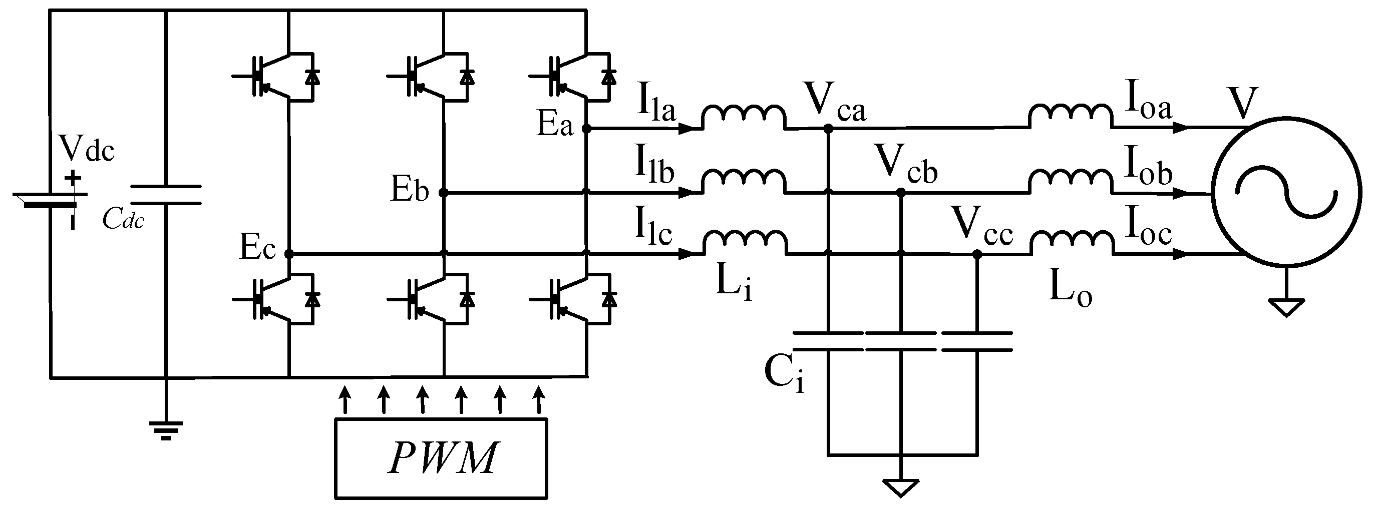
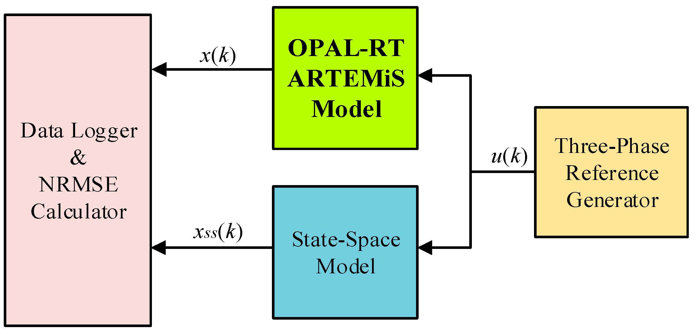
As the open-loop models do not contain any controller to regulate the current spikes nor phase deviations, this could cause inverters to trip or even having a safety issue if the models are validated in a physical experiment. Thus, their validation can only be performed using real-time simulation tools. To validate the accuracy of the mathematical model of an inverter connected to the main grid, the simulation of the circuit shown in Figure 2 was computed in parallel with its mathematical model ${\mathrm{G}}_{\mathrm{i}}\left(\mathrm{z}\right)$. 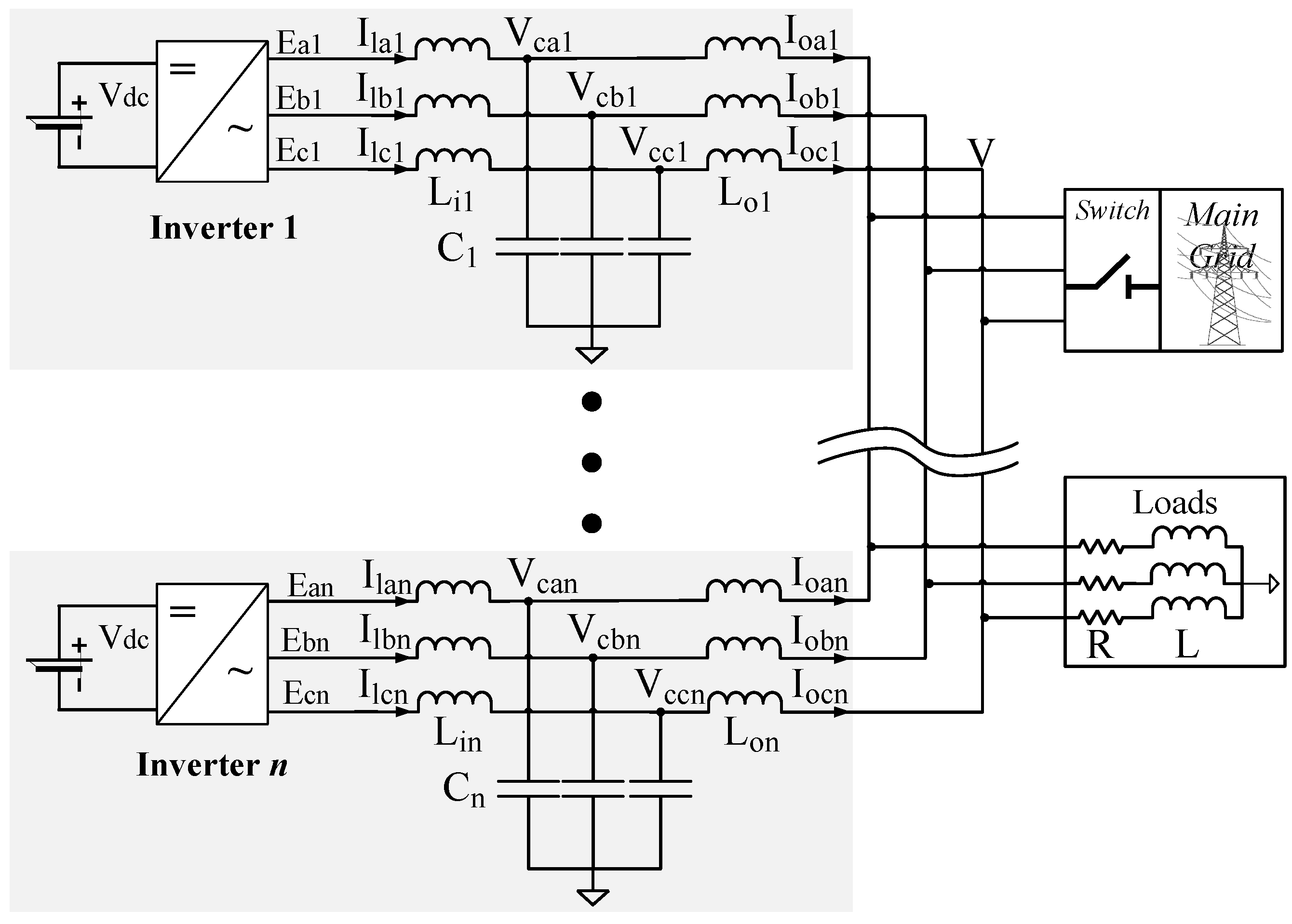Similarly, to validate the accuracy of the mathematical model of an islanded microgrid, the simulation of the microgrid scheme shown in Figure 3 was computed in parallel with its mathematical model ${\mathrm{G}}_{\mathsf{\mu }\mathrm{G}}\left(\mathrm{z}\right)$. For both validations (grid-connected and islanded mode), the same input signal was used on the mathematical model and the simulated circuit as shown in Figure 5. The three-phase reference generator produces step changes in amplitude in order to compare transient responses. Each inverter was simulated using an OPAL OP5700 real-time simulator with the ARTEMiS library for power electronics devices from Opal-RT Technologies™ [31]. The mathematical solver of this library runs accurate simulations of power electronics devices, such as the IGBT transistors used in three-phase inverters.

3.1.1. Grid-Connected Inverter Model

To validate the mathematical model (13), the LCL component values for Inverter 1 were used. Once the Inverter 1 model was validated, it was assumed that (13) was adequate in describing the dynamics of any grid-connected inverter such as Inverters 2 or 3.

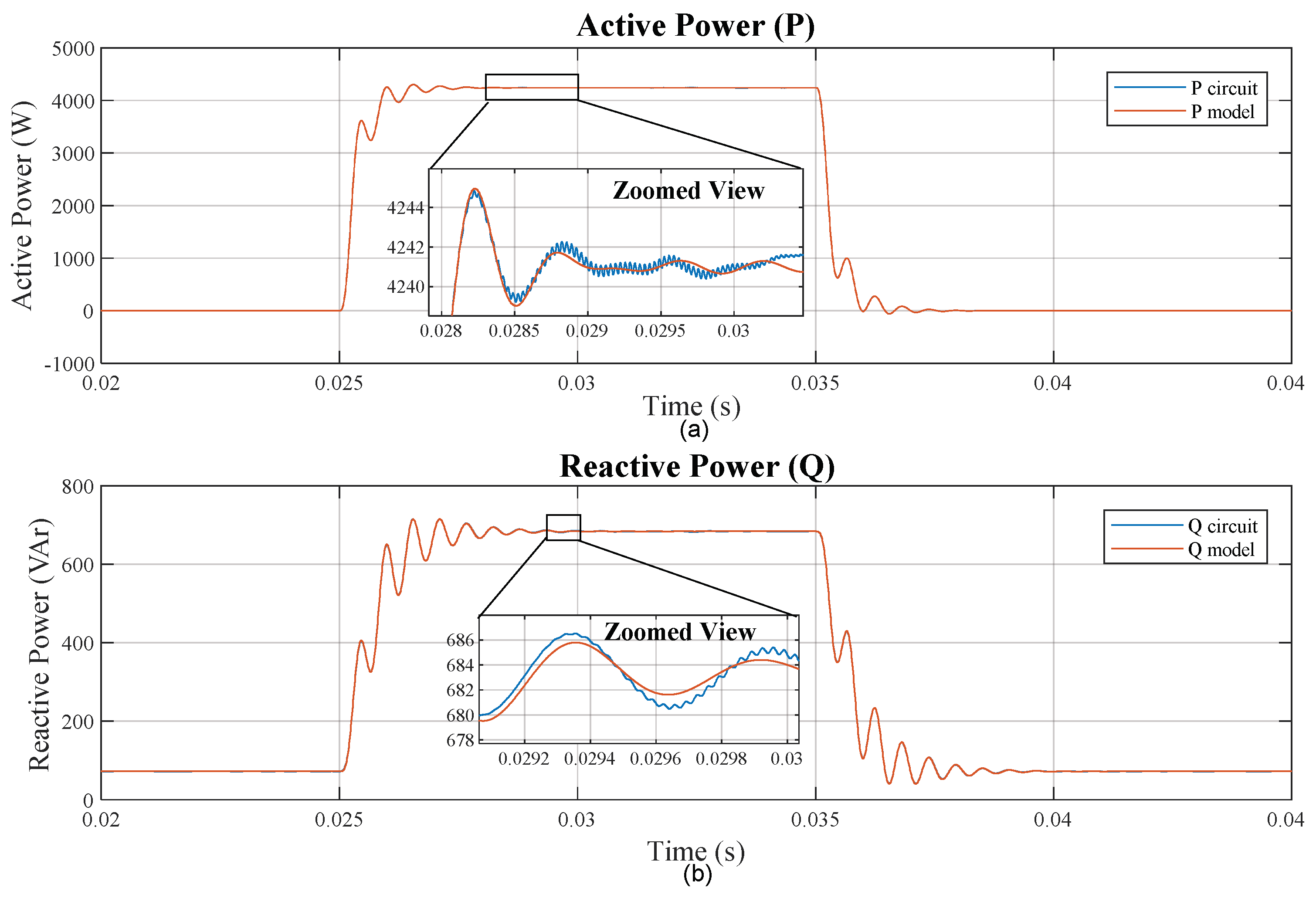
For this experiment, the inverter output voltage $\mathrm{E}$ and main grid voltage ${\mathrm{V}}_{\mathrm{g}}$ started with the same nominal amplitude and phase. At $\mathrm{t}=0.025 \mathrm{s}$, the inverter output amplitude was duplicated to a peak value of $240\sqrt{2}$ and returned to the original value at $\mathrm{t}=0.035 \mathrm{s}$. Figure 6 shows the active and reactive power values for the mathematical model and circuit. Zoomed views in Figure 6 show that active and reactive power for the mathematical model and circuit have similar dynamics. However, there are small high-frequency oscillations in the power of the circuit. These oscillations are generated by IGBT transistor switching at a frequency of $10\mathrm{kHz}$.

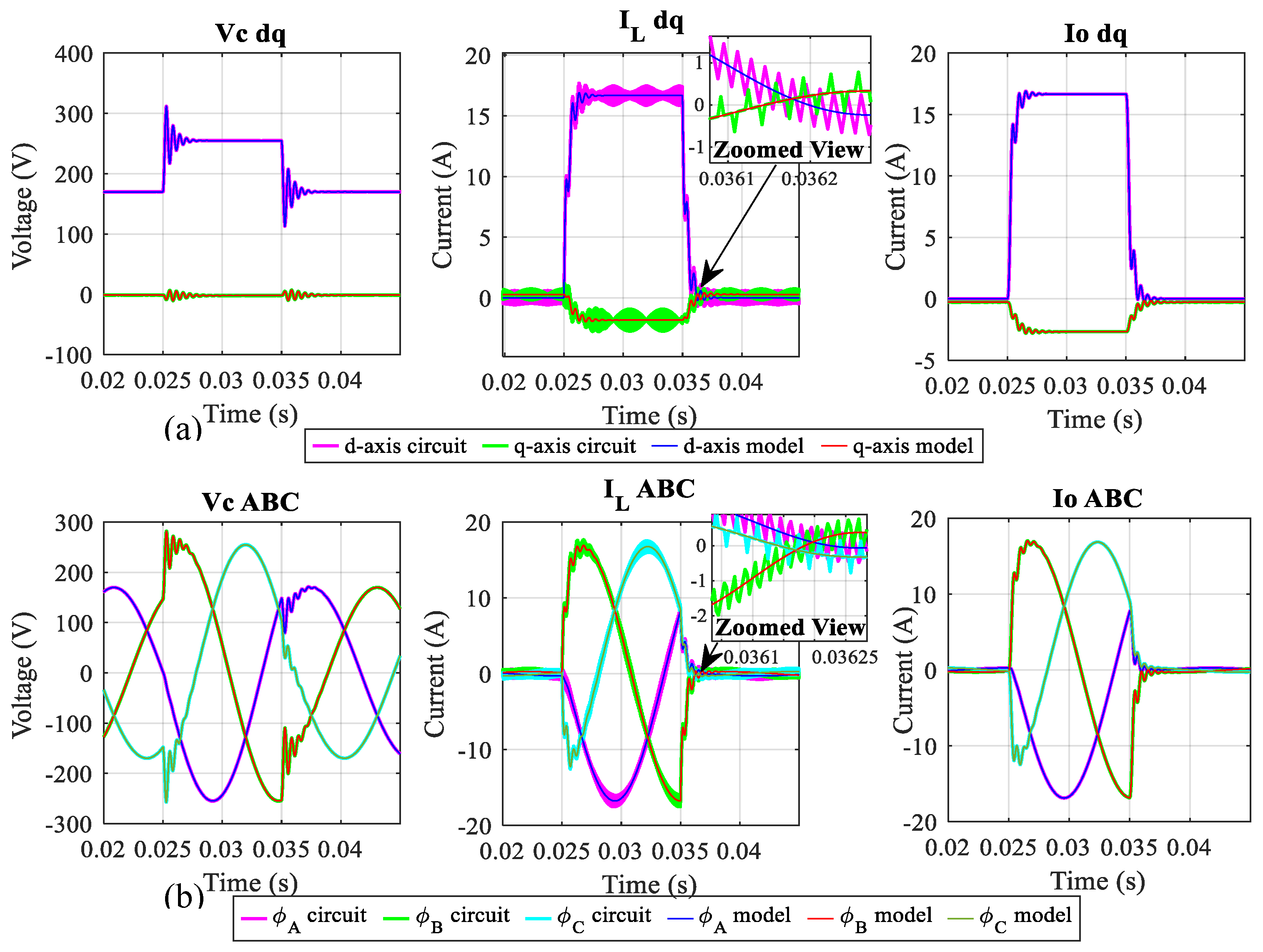
Figure 7 shows the state vector waveforms in the dq frame and ABC frame. Zoomed views also show the current switching oscillations in the input inductor. However, state vector dynamics show similar behavior in steady state and during transient response.

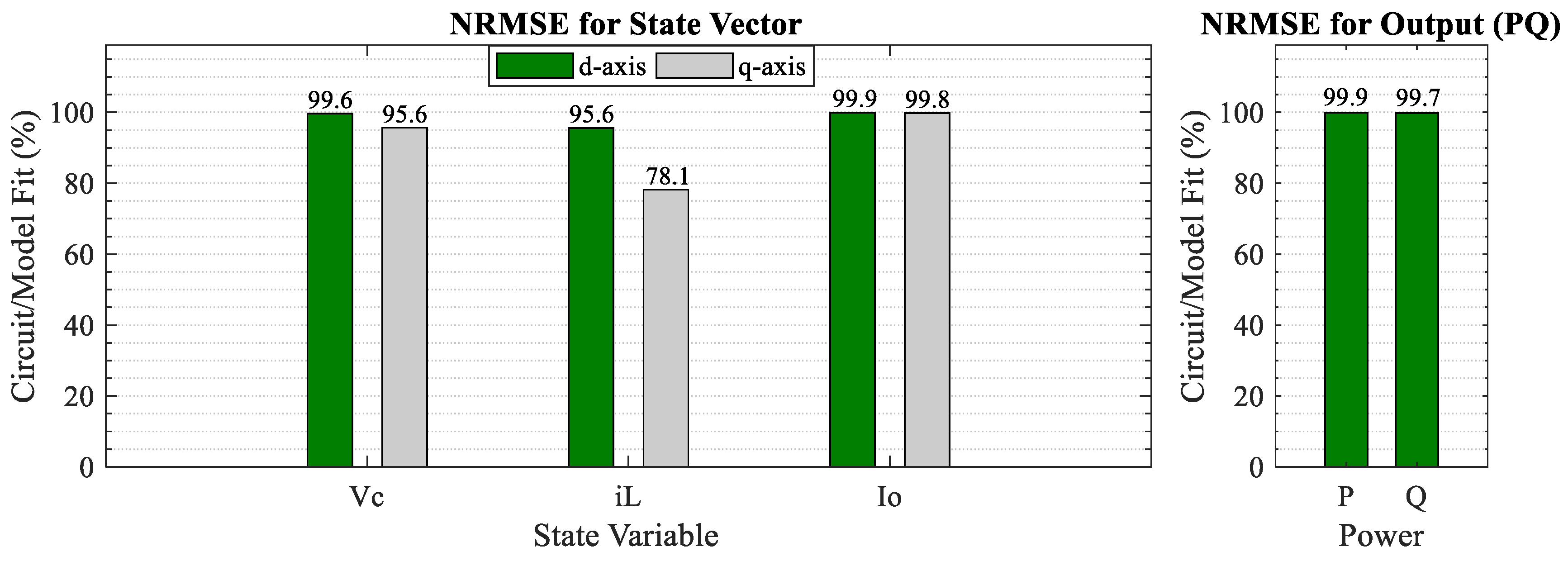
The NRMSE value was also analyzed for the shared power and the state vector in the dq frame. Figure 8 shows that the fitting values are above 95% in all the state variables except the input inductor current, which is about 78% on the q component of the input inductor current. This is produced by the 10 KHz switching noise of the PWM signal, which was not considered in the proposed model. These results validate the accuracy of the proposed model for the grid-connected inverter.

Open-loop eigenvalues of nominals ${\mathrm{G}}_1\left(\mathrm{z}\right)$, ${\mathrm{G}}_2\left(\mathrm{z}\right)$, and ${\mathrm{G}}_3\left(\mathrm{z}\right)$ and their variations are shown in Figure 9. As seen in the zoomed view, the eigenvalues remain inside the unit circle, which implies that all the inverters were stable in grid-connected mode without a controller. However, after analyzing the stability margins, none of the open-loop models were closed-loop stable using unit feedback.

Singular value diagrams of the nominal ${\mathrm{G}}_1\left(\mathrm{z}\right)$, ${\mathrm{G}}_2\left(\mathrm{z}\right)$, and ${\mathrm{G}}_3\left(\mathrm{z}\right)$ and their variations are shown in Figure 10. According to these diagrams, frequency responses of Inverters 2 and 3 are similar, with variations on their resonant and crossover frequencies. Moreover, Inverter 1 has the fastest dynamics followed by Inverters 2 and 3, respectively.

3.1.2. Islanded Microgrid Model

For the islanded mode, the scenario was simulated using an OPAL OP5700 real-time simulator with the ARTEMiS library for power electronics devices [31]. The ARTEMiS library was used to perform accurate simulations that considered the switching behavior of power electronic devices. To validate the mathematical model, the LCL component values from Table 1 were used. For this experiment, the output voltage of the three inverters and the main grid started with the same nominal amplitude and phase. At $\mathrm{t}=0.025 \mathrm{s}$, the inverters’ output amplitude was duplicated to a peak value of $240\sqrt{2}$ and returned to the original value at $\mathrm{t}=0.035 \mathrm{s}$. 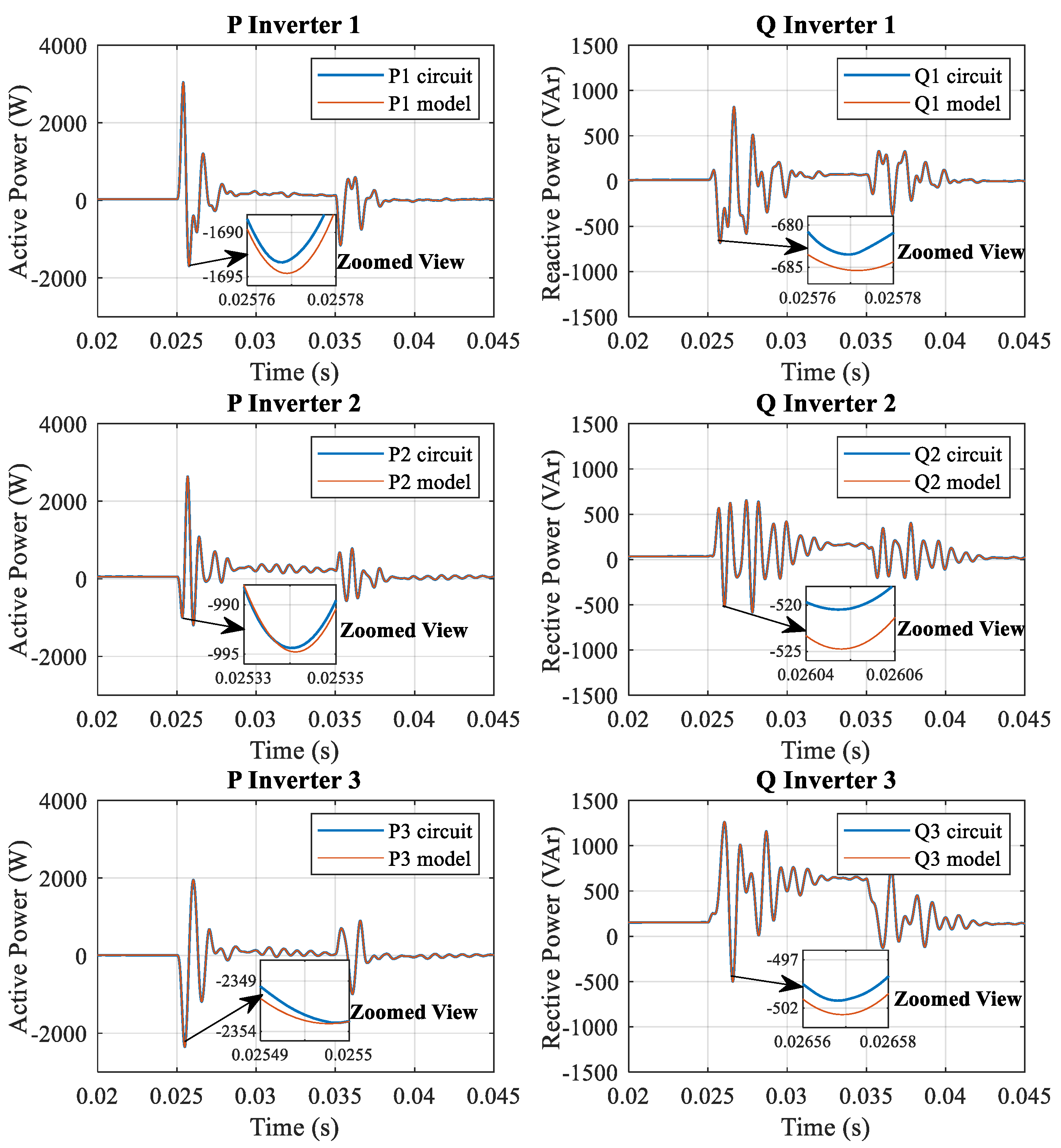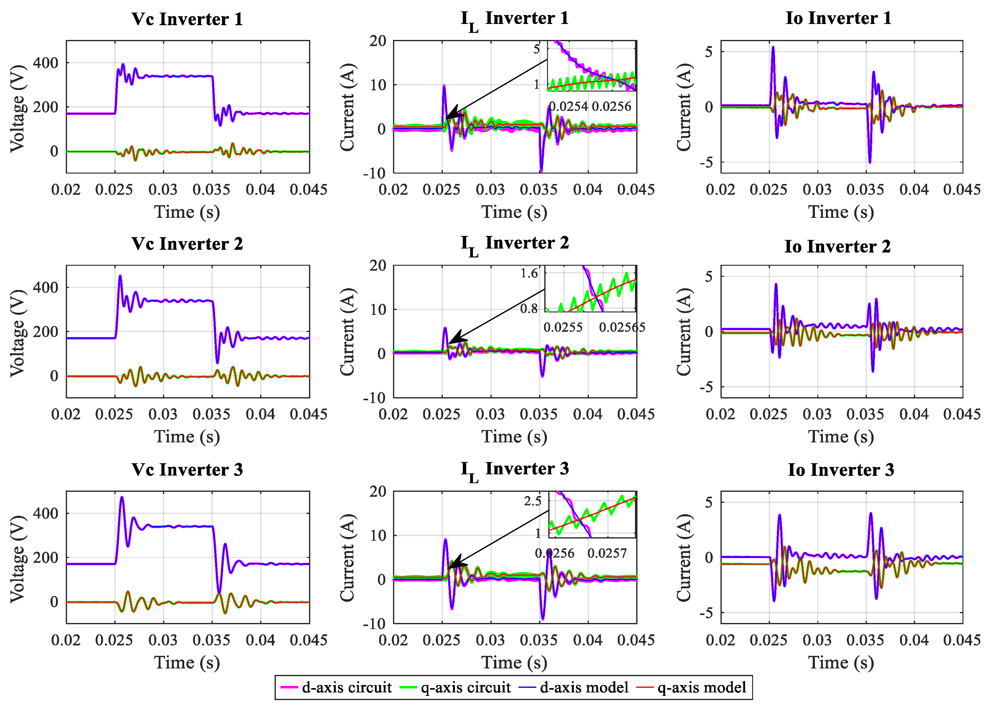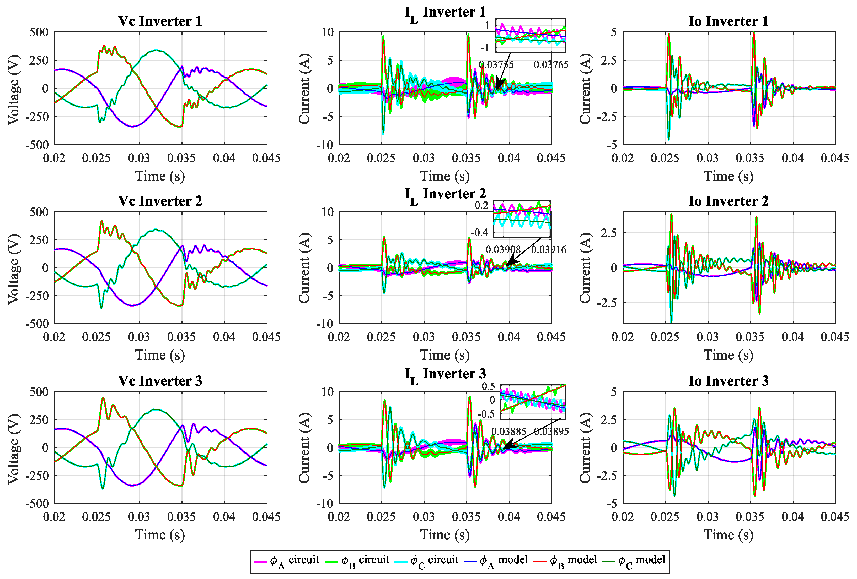Figure 11 shows the active and reactive power waveforms for the mathematical model and circuit. State vector waveforms in the dq frame are shown in Figure 12 and in the ABC frame in Figure 13. The active and reactive power for the mathematical model and circuit have similar dynamics. As detailed in zoomed views, input inductor currents showed switching oscillations. These oscillations were caused by the IGBT transistors switching at a frequency of $10\mathrm{kHz}$. However, state vector dynamics show similar behavior in steady state and during transient response.

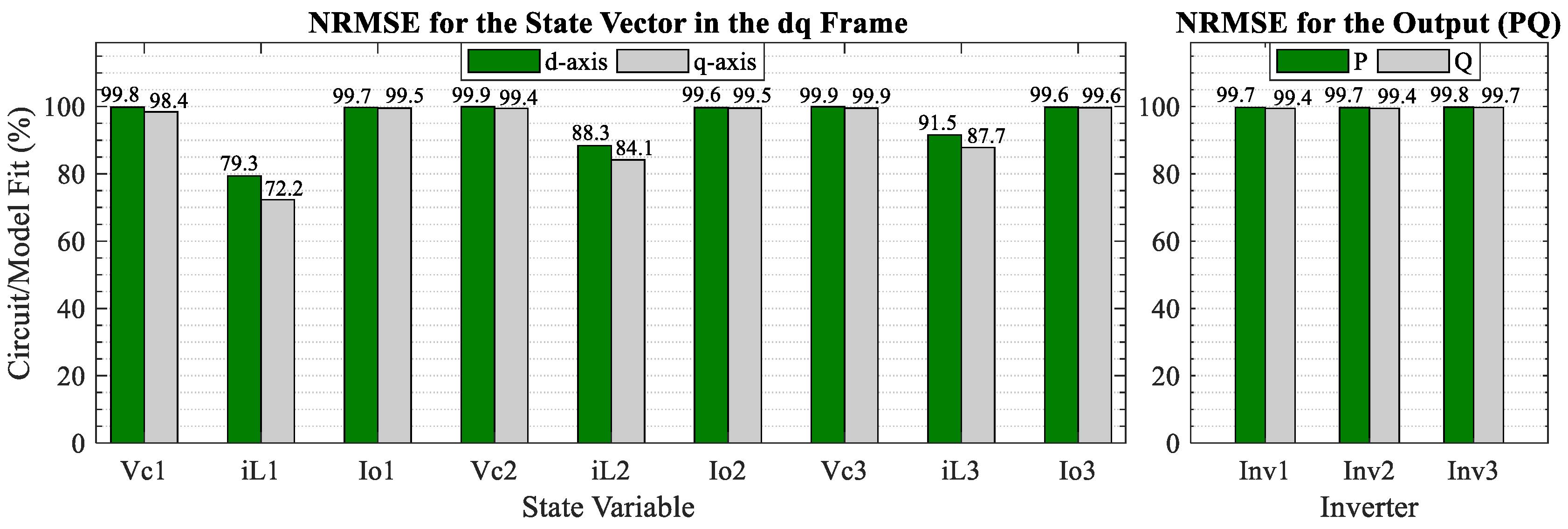
The NRMSE value was also analyzed for the shared power and the state vector in the dq frame. Figure 14 shows that fitting values are above 98% in all the state variables except for the input inductor currents, which decrease due to the presence of the 10 kHz PWM switching. These results validate the accuracy of the proposed model for the islanded microgrid.

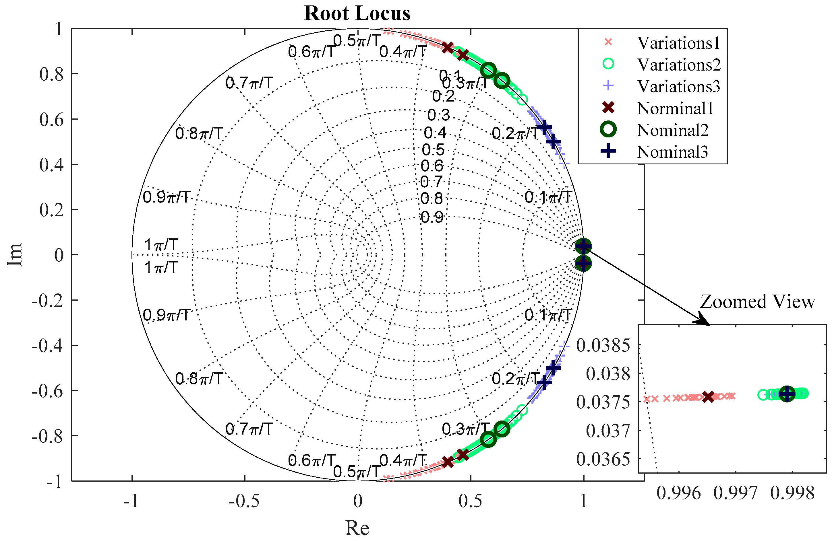
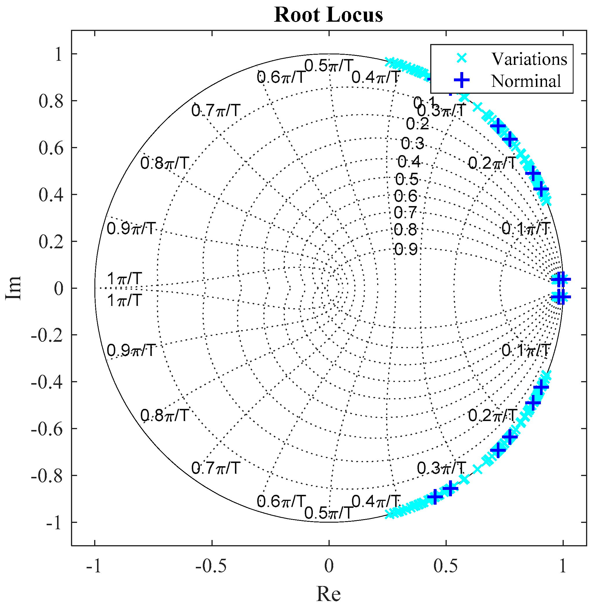
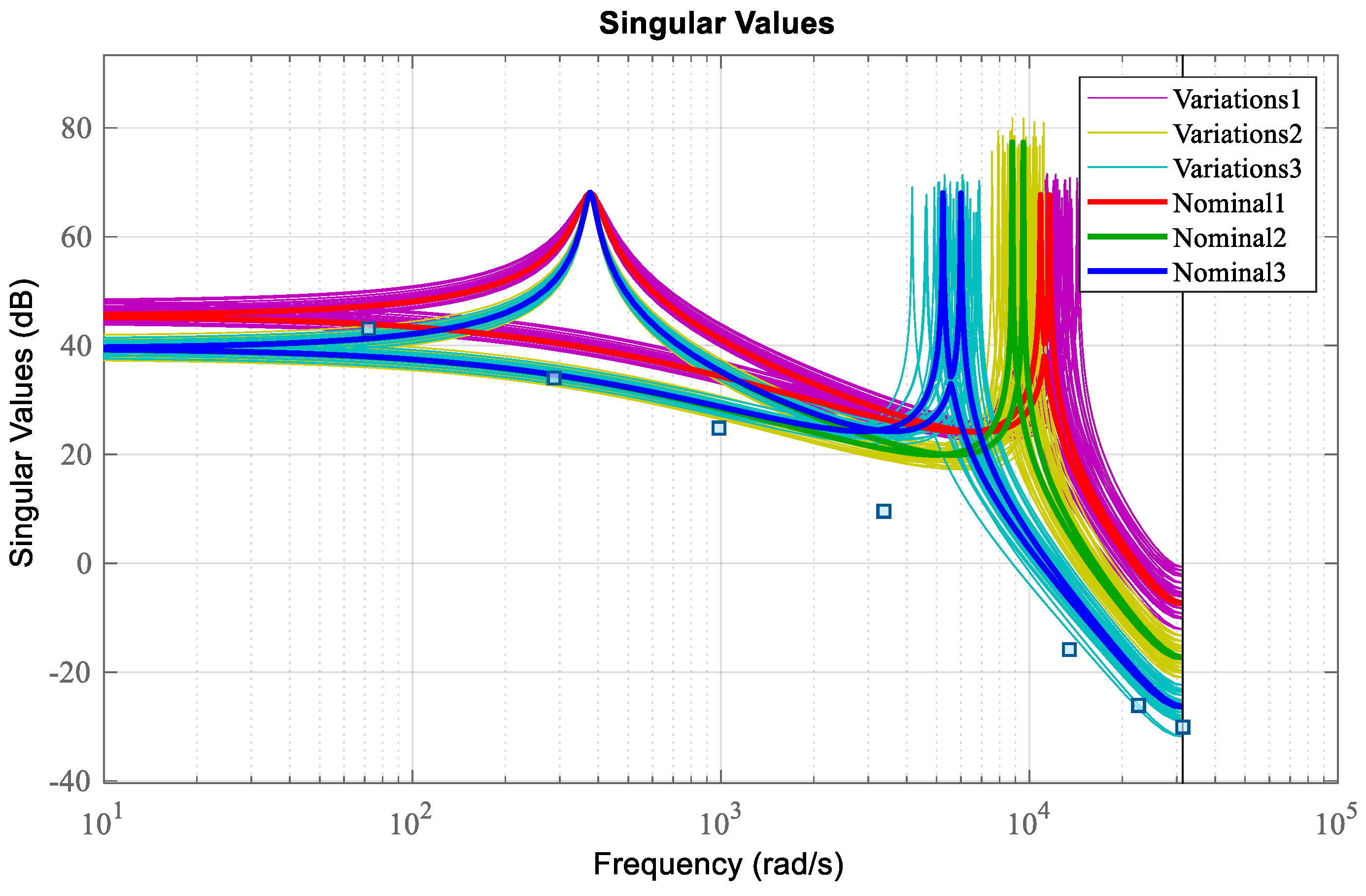
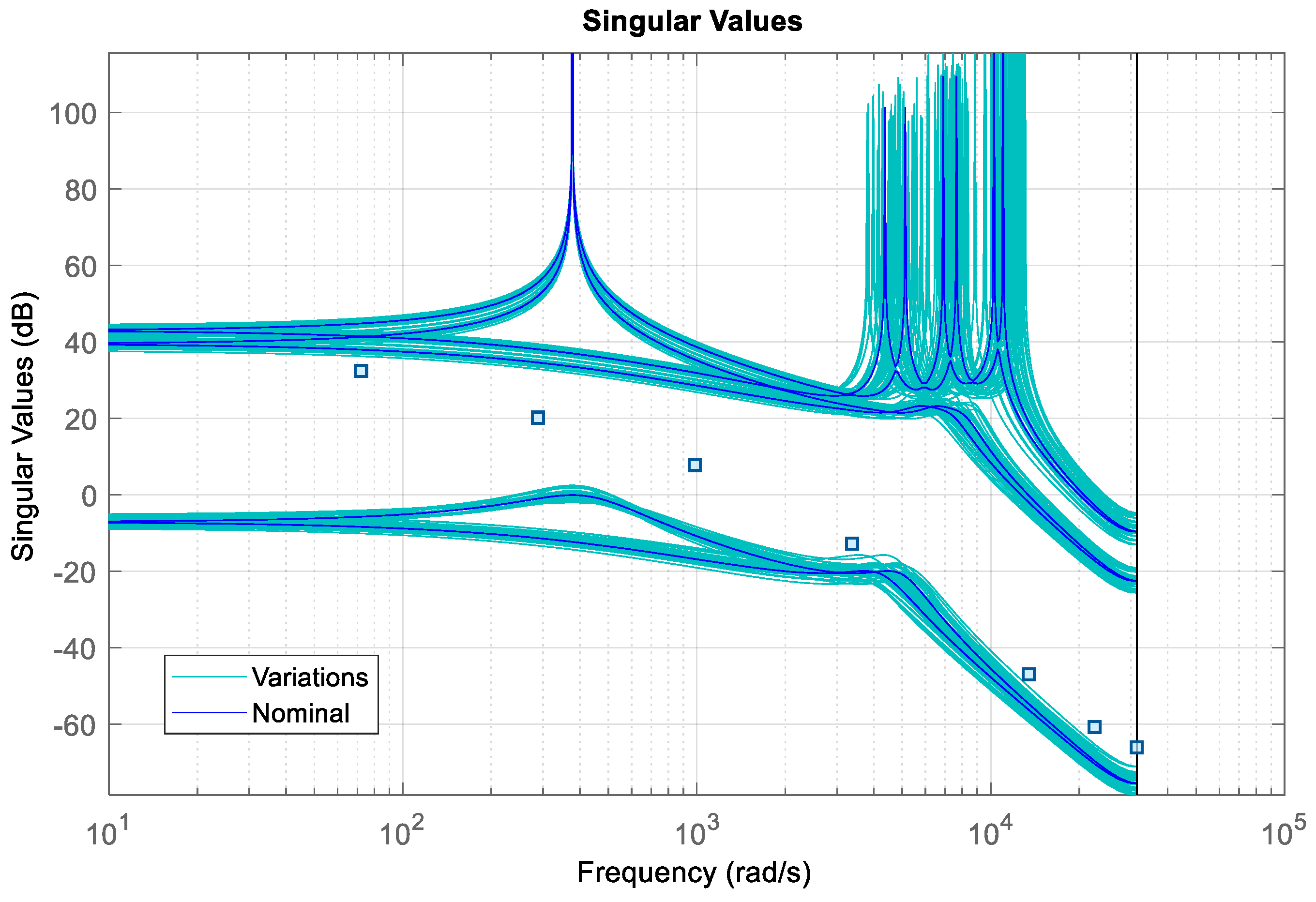
Open-loop eigenvalues of ${\mathrm{G}}_{\mathsf{\mu }\mathrm{G}}\left(\mathrm{z}\right)$ and its variations are shown in Figure 15. All the eigenvalues remain inside the unit circle, which implies that the open-loop microgrid is stable in grid-connected mode without a controller. However, after analyzing stability margins, none of the open-loop models were closed-loop stable using a unit feedback. Finally, the singular value diagrams of the nominal ${\mathrm{G}}_{\mathsf{\mu }\mathrm{G}}\left(\mathrm{z}\right)$ and its variations are shown in Figure 16. These diagrams show similar behavior compared to Figure 10. However, there is an additional response below $0\mathrm{dB}$ that is related to the RL load.

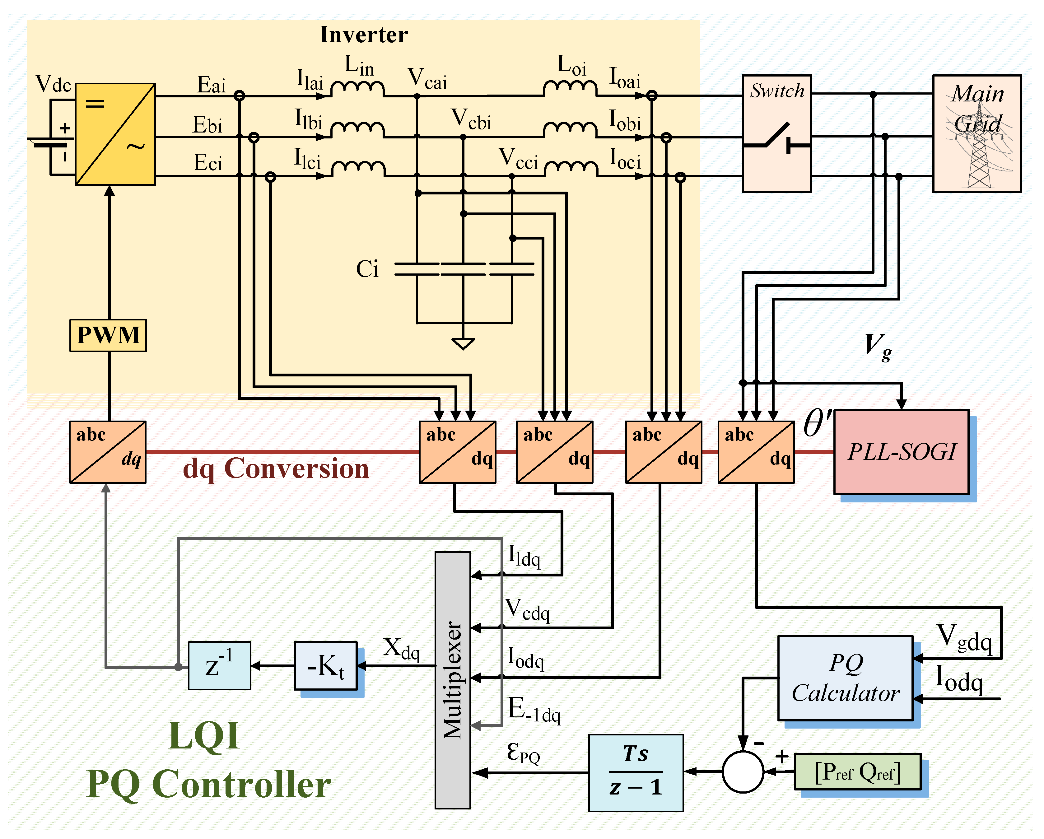
3.2. Scenario 2: Grid-Connected LQI Power Controller

The power controller for the grid-connected inverter was developed using (18) with the component values of Inverter 1 from Table 1. The control scheme is shown in Figure 17. To synchronize each inverter with the AC bus, a second order generalized integrator (SOGI-PLL) is implemented as shown in Figure 23.

3.2.1. LQI Controller

The LQI controller is designed to minimize the tracking error by computing the integral of the error vector $\mathsf{\epsilon }={{\displaystyle \sum }}_{\mathrm{i}}\left({\mathrm{Cx}}_{\mathrm{i}}{-\mathrm{r}}_{\mathrm{i}}\right)$. The augmented model that includes the tracking error is given by

$$\stackrel{{\overline{\mathrm{X}}}_{\mathrm{T}}[\mathrm{k}+1]}{\overbrace{\left[\begin{array}{c}{\mathrm{X}}_{\mathrm{T}}\left[\mathrm{k}+1\right]\\ \mathsf{\epsilon }\left[\mathrm{k}+1\right]\end{array}\right]}}=\stackrel{{\overline{\mathrm{A}}}_{\mathrm{T}}}{\overbrace{\left[\begin{array}{cc}{\mathrm{A}}_{\mathrm{T}}& 0_{6\times 2}\\ {\mathrm{T}}_{\mathrm{s}}\mathrm{C}& {\mathrm{I}}_{2\times 2}\end{array}\right]}}\stackrel{{\overline{\mathrm{X}}}_{\mathrm{T}}\left[\mathrm{k}\right]}{\overbrace{\left[\begin{array}{c}{\mathrm{X}}_{\mathrm{T}}\left[\mathrm{k}\right]\\ \mathsf{\epsilon }\left[\mathrm{k}\right]\end{array}\right]}}+\stackrel{{\overline{\mathrm{B}}}_{1\mathrm{T}}}{\overbrace{\left[\begin{array}{c}{\mathrm{B}}_{1\mathrm{T}}\\ 0_{2\times 2}\end{array}\right]}}{\mathrm{E}}_{\mathrm{dq}}\left[\mathrm{k}\right]+\stackrel{{\overline{\mathrm{B}}}_{\mathrm{int}}}{\overbrace{\left[\begin{array}{c}{0}_{8\times 2}\\ {\mathrm{I}}_{2\times 2}\end{array}\right]}}\mathrm{r}\left[\mathrm{k}\right]+\stackrel{{\overline{\mathrm{B}}}_{2\mathrm{T}}}{\overbrace{\left[\begin{array}{c}{\mathrm{B}}_{2\mathrm{T}}\\ 0_{2\times 2}\end{array}\right]}}{\mathrm{V}}_{\mathrm{gdq}}\left[\mathrm{k}\right]$$

(29)

Defining the control law as ${\mathrm{E}}_{\mathrm{dq}}=-{\mathrm{K}}_{\mathrm{t}}{\overline{\mathrm{X}}}_{\mathrm{T}}$, the closed-loop model is given by

$${\overline{\mathrm{X}}}_{\mathrm{T}}[\mathrm{k}+1]={({\overline{\mathrm{A}}}_{\mathrm{T}}-{\overline{\mathrm{B}}}_{1\mathrm{T}}{\mathrm{K}}_{\mathrm{t}})}^{-1}{\overline{\mathrm{X}}}_{\mathrm{T}}\left[\mathrm{k}\right]+{\overline{\mathrm{B}}}_{\mathrm{int}}\mathrm{r}\left[\mathrm{k}\right]+{\overline{\mathrm{B}}}_{2\mathrm{T}}{\mathrm{V}}_{\mathrm{gdq}}\left[\mathrm{k}\right]$$

(30)

To compute the LQI controller, the following cost function is defined:

$$\mathrm{J}\left[{\mathrm{k}}_0\right]=\sum _{\mathrm{k}={\mathrm{k}}_0}^{\mathrm{T}}\{{(\mathrm{C}{\overline{\mathrm{X}}}_{\mathrm{T}}\left[\mathrm{k}\right]-\mathrm{r}\left[\mathrm{k}\right])}^{\mathrm{T}}{\mathrm{Q}}_{\mathrm{p}}(\mathrm{C}{\overline{\mathrm{X}}}_{\mathrm{T}}\left[\mathrm{k}\right]-\mathrm{r}\left[\mathrm{k}\right])+{\mathrm{E}}_{\mathrm{dq}}^{\mathrm{T}}\left[\mathrm{k}\right]{\mathrm{R}}_{\mathrm{p}}{\mathrm{E}}_{\mathrm{dq}}\left[\mathrm{k}\right]\}$$

(31)

where Q_p and R_p are some positive-definite and semi-positive-definite weighting matrices, respectively. The output matrix results by the augmentation of (17):

$$\mathrm{C}=\frac{3}{2}\left[\begin{array}{cccccccccc}0& 0& 0& 0& {\overline{\mathrm{V}}}_{\mathrm{gd}}& 0& 0& 0& 0& 0\\ 0& 0& 0& 0& 0& -{\overline{\mathrm{V}}}_{\mathrm{gd}}& 0& 0& 0& 0\end{array}\right]$$

(32)

The LQI feedback matrix K_t is given by

$${\mathrm{K}}_{\mathrm{t}}={({\overline{\mathrm{B}}}_{1\mathrm{T}}^{\mathrm{T}}{\mathrm{S}}_{\mathrm{p}}{\overline{\mathrm{B}}}_{1\mathrm{T}}+{\mathrm{R}}_{\mathrm{p}})}^{-1}{\overline{\mathrm{B}}}_{1\mathrm{T}}^{\mathrm{T}}\mathrm{S}{\overline{\mathrm{A}}}_{\mathrm{T}}$$

(33)

where S_p is the solution to the algebraic Ricatti equation [32]:

$${\mathrm{S}}_{\mathrm{p}}={\overline{\mathrm{A}}}_{\mathrm{T}}^{\mathrm{T}}{\mathrm{S}}_{\mathrm{p}}({\overline{\mathrm{A}}}_{\mathrm{T}}-{\overline{\mathrm{B}}}_{1\mathrm{T}}{\mathrm{K}}_{\mathrm{t}})+{\mathrm{C}}^{\mathrm{T}}{\mathrm{Q}}_{\mathrm{p}}\mathrm{C}$$

(34)

3.2.2. Performance Analysis

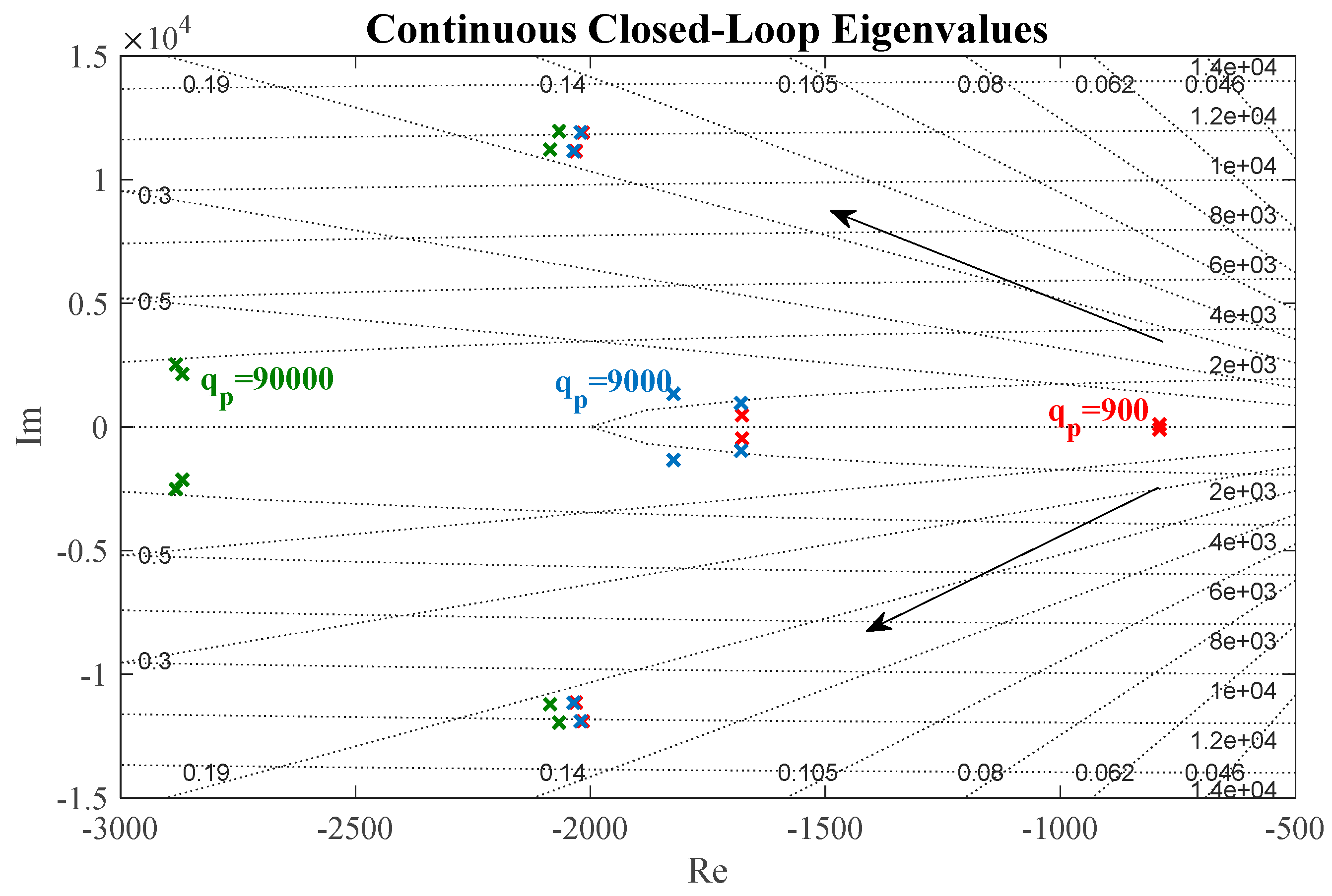
To identify the adequate values of Q_p and R_p, a stability analysis was performed using open-loop singular value diagrams, closed-loop eigenvalue plots, and closed-loop step responses. It was desired that the closed-loop system reached a steady state in less than 0.005s with a damping ratio less than 0.7. The closed-loop eigenvalues are given by

$$\mathsf{\lambda }\{{(\mathrm{I}+\mathsf{\Lambda }(\mathrm{z}\left)\right)}^{-1}\}=\mathsf{\lambda }\{{\overline{\mathrm{A}}}_{\mathrm{T}}-{\overline{\mathrm{B}}}_{\mathrm{T}}{\mathrm{K}}_{\mathrm{t}}\}$$

(35)

For illustration purposes, the discrete closed-loop eigenvalues were transformed into continuous time using ${\mathrm{z}=\mathrm{e}}^{\mathrm{sT}}.$ Closed-loop eigenvalues were calculated for different values of ${\mathrm{q}}_{\mathrm{p}}$ in ${\mathrm{Q}}_{\mathrm{p}}=\mathrm{diag}\left(\left[\begin{array}{cccccccccc}1& 1& 1& 1& 100& 100& 1& 1& {\mathrm{q}}_{\mathrm{p}}& {\mathrm{q}}_{\mathrm{p}}\end{array}\right]\right)$ and ${\mathrm{R}}_{\mathrm{p}}{=\mathrm{r}}_{\mathrm{p}}{\mathrm{I}}_{2\times 2}$. From the eigenvalue plot shown in Figure 18, it can be noticed that the eigenvalues with ${\mathrm{q}}_{\mathrm{p}}=9000$ are more suitable to fulfill design requirements.

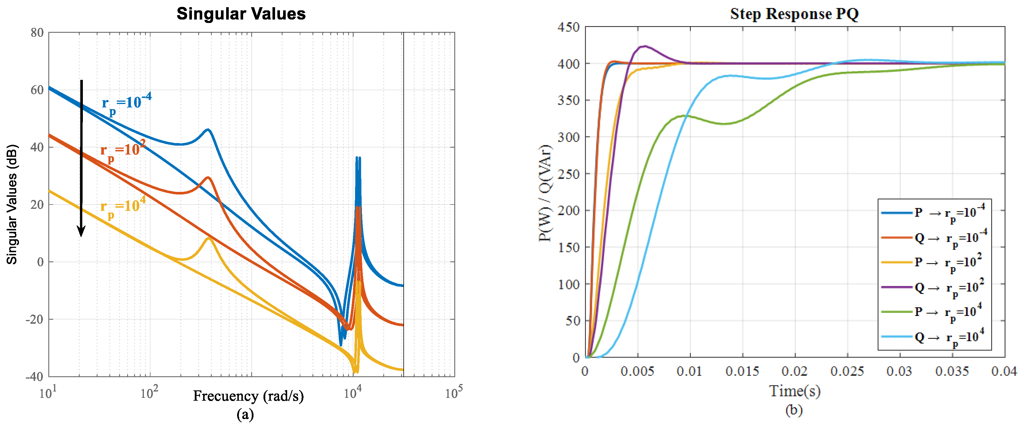
The open-loop transfer function is given by

$$\mathsf{\Lambda }\left(\mathrm{z}\right)={\mathrm{K}}_{\mathrm{t}}{(\mathrm{zI}-{\overline{\mathrm{A}}}_{\mathrm{T}})}^{-1}{\overline{\mathrm{B}}}_{1\mathrm{T}}$$

(36)

After selecting ${\mathrm{Q}}_{\mathrm{p}}$, the singular value plot and the step-response plot were analyzed by varying ${\mathrm{r}}_{\mathrm{p}}$. For this analysis, it was desired to attenuate the high-frequency noise in the power measurement. The high-frequency noise is considered a disturbance in the process since it is produced by the transistors. To attenuate the process noise, it is desired for the open-loop SVD bandwidth to be as high as possible without affecting the step-response requirements [25]. Figure 19 shows that a suitable response is achieved for ${\mathrm{r}}_{\mathrm{p}}$ = 0.0001. The resulting state-feedback matrix is given by

$${\mathrm{K}}_{\mathrm{t}}=\left[\begin{array}{cccccccccc}-0.547& -0.043& 9.855& 0.372& 4.348& -0.140& 0.666& 0.018& -58.172& -6.685\\ 0.043& -0.547& -0.372& 9.855& 0.140& 4.348& -0.018& 0.666& -6.685& 58.172\end{array}\right]$$

(37)

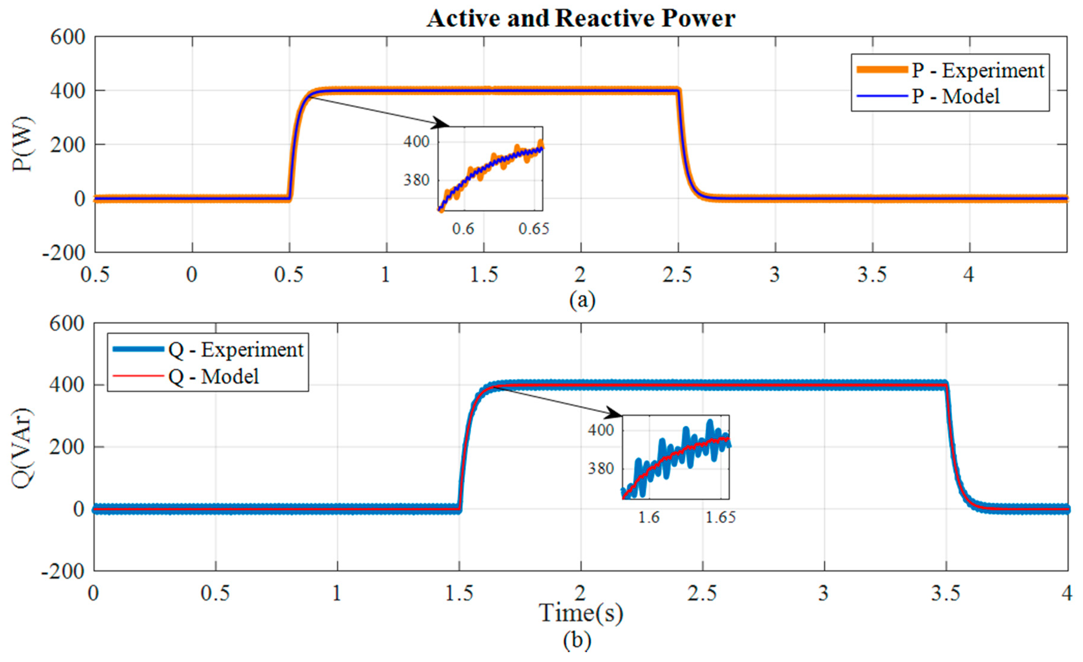
3.2.3. Experimental Results

To assess the performance of the proposed model and to validate the closed-loop model, the experimental setup from Figure 4 was used. The experimental response was compared against the mathematical response of the closed-loop model under a step reference of 400 W and 400 VAr. As the closed-loop inputs from (30) include the grid voltage, the acquired voltage measurement from the power authority was transformed to the dq frame and was used as the input of the closed-loop mathematical model.

Experimental and mathematical values for the active and reactive power are shown in Figure 20. As the power measurement contains high-frequency noise generated by the PWM switching, a first-order low-pass filter with a bandwidth of ${\mathsf{\omega }}_{\mathrm{c}}=10\mathrm{rad}/\mathrm{s}$ was used. Notice that, unlike classical droop controllers, this filter is only used for visualization purposes and is not included in the control loop.

Results from Figure 20 demonstrate that the performance of the proposed controller is adequate. Moreover, the NRMSE for the active power is 98.89% and 97.23% for the reactive power. This demonstrates that the mathematical closed-loop model and that the experimental results are alike.

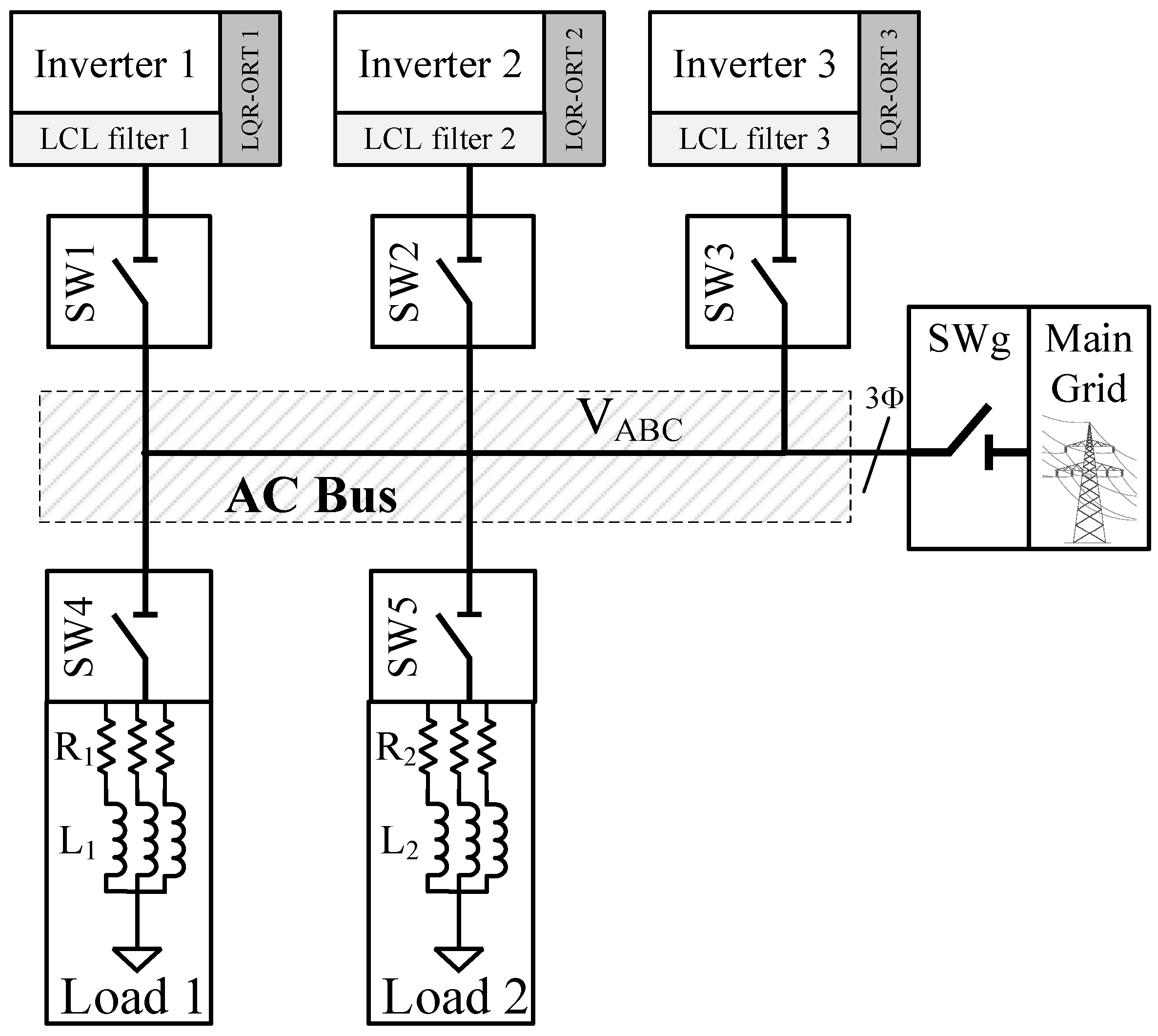
3.3. Scenario 3: Islanded PQ/Vdq LQI-Based Droop–Boost Controller

To demonstrate the effectiveness and the applicability of the islanded model, a microgrid scenario with three inverter-based generators and two loads was proposed, as shown in Figure 21. Connection switches were located at the output of each inverter, at the input to each load, and at the point of connection with the main grid. Without loss of generality, all three inverters had the same LCL filter components to simplify the design procedure. However, the design procedure shown in this section is also suitable for microgrids with different LCL filter components. The parameter specification for the microgrid scenario is shown in

Table 2. Parameter specifications for the microgrid scenario.

Parameter	Symbol	Value
Grid Voltage	${\mathrm{V}}_{\mathrm{g}}$	$120{\mathrm{V}}_{\mathrm{RMS}}$
DC Bus Voltage	${\mathrm{V}}_{\mathrm{dc}}$	$350\mathrm{V}$
Grid Frequency	${\mathrm{f}(\mathsf{\omega }}_{\mathrm{c}})$	$60\mathrm{Hz}(376.99\mathrm{rad}/\mathrm{s})$
Output Inductance	${\mathrm{L}}_{\mathrm{o}}$	$1.8\mathrm{mH}$
Input Inductance	${\mathrm{L}}_{\mathrm{i}}$	$1.8\mathrm{mH}$
Filter Capacitance	$\mathrm{C}$	$8.8\mathsf{\mu }\mathrm{F}$
PWM Frequency	${\mathrm{f}}_{\mathrm{PWM}}$	$10\mathrm{kHz}$
Sampling Period	${\mathrm{T}}_{\mathrm{s}}$	$100\mathsf{\mu }\mathrm{s}$
Load 1, Load 2	${\mathrm{R}}_1{,\mathrm{L}}_1$	$171.43\mathsf{\Omega },0.46\mathrm{H}$

.

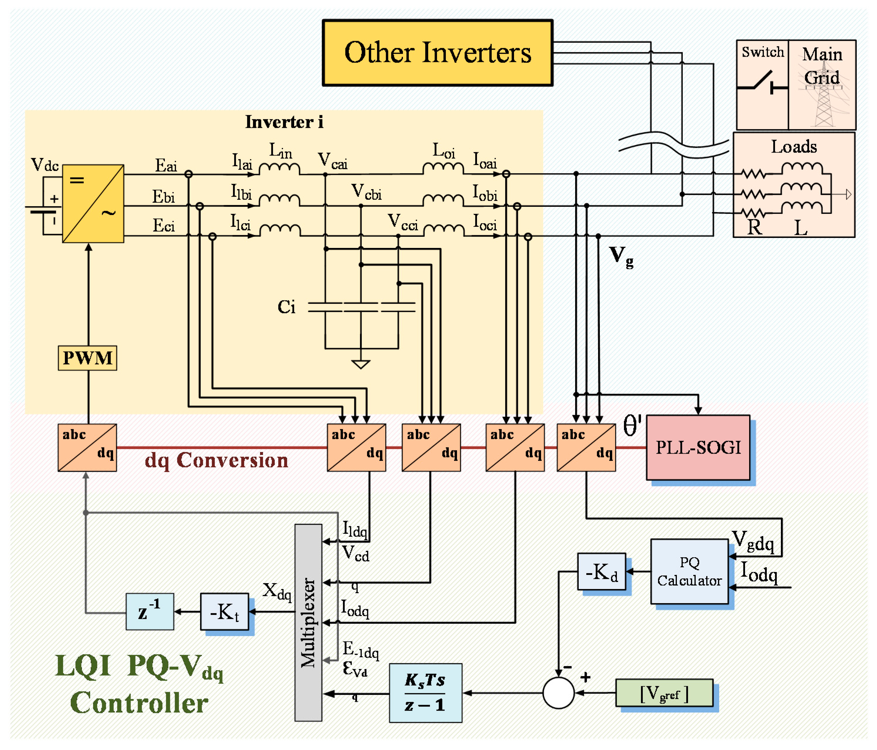
3.3.1. Controller Design

The controller presented in this section is designed for each inverter independently. The control scheme for one inverter is shown in Figure 22. Each controller contains an internal LQI controller to regulate the output voltage V_cdq. The voltage reference of the LQI controller ${\mathrm{V}}_{\mathrm{cref}}$ is generated by the PQ/Vdq droop–boost controller according to the active and reactive power demanded by the load. The AC bus reference is set to nominal values such that ${\mathrm{V}}_{\mathrm{gref}}=\left[\begin{array}{cc}{\overline{\mathrm{V}}}_{\mathrm{gd}}& 0\end{array}\right]$.

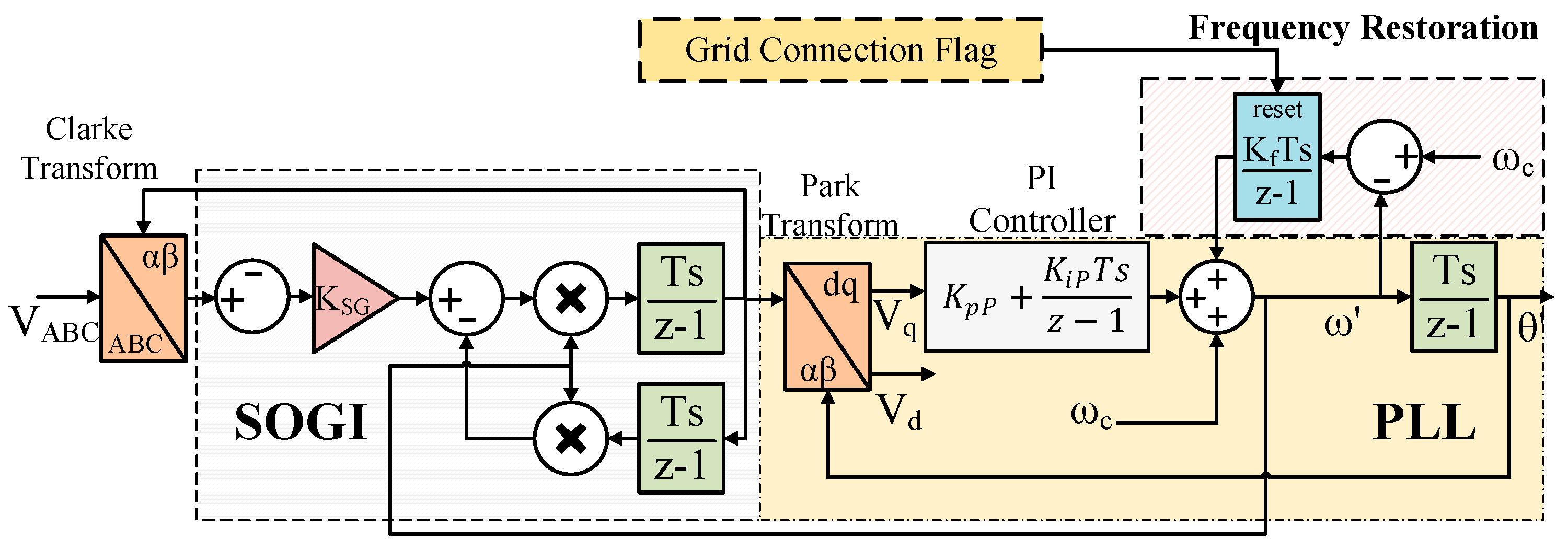
To synchronize each inverter with the AC bus, a second order generalized integrator (SOGI-PLL) is implemented as shown in Figure 23 [33]. The output of the SOGI-PLL is used to perform the dq transformation of the input and output signals of the LQI controller. When the grid connection is lost, the operating frequency of the microgrid drops and the frequency restoration loop is activated. The frequency restoration loop integrates the frequency error and compensates the PLL operating frequency ${\mathsf{\omega }}^{\prime }$. This way, the microgrid frequency returns to nominal values in islanded mode. The expression of the output frequency of the SOGI-PLL with the proposed frequency restoration loop is given by

$${\mathsf{\omega }}^{\prime }{=\mathrm{V}}_{\mathrm{q}}\left({\mathrm{K}}_{\mathrm{pP}}+\frac{{\mathrm{K}}_{\mathrm{iP}}{\mathrm{T}}_{\mathrm{s}}}{\mathrm{z}-1}\right){+\mathsf{\omega }}_{\mathrm{c}}+\frac{{\mathrm{F}}_{\mathrm{g}}{\mathrm{K}}_{\mathrm{f}}{\mathrm{T}}_{\mathrm{s}}}{\mathrm{z}-1}\left({\mathsf{\omega }}^{\prime }{-\mathsf{\omega }}_{\mathrm{c}}\right)$$

(38)

where ${\mathrm{F}}_{\mathrm{g}}$ is zero when the grid connection is lost and one when the grid is engaged. When synchronized, it may be assumed that ${\mathrm{V}}_{\mathrm{gq}}=0$. Thus, in steady state ${\mathsf{\omega }}^{\prime }\approx {\mathsf{\omega }}_{\mathrm{c}}$.

3.3.2. LQI Controller

Similar to Section 3.2.2, the LQI controller was designed using the augmented model (29). However, the output matrix is now defined to track the voltage error instead of output power as follows:

$$\mathrm{C}=\left[\begin{array}{ccccccccc}1& 0& 0& 0& 0& 0& 0& 0& 0\\ 0& 1& 0& 0& 0& 0& 0& 0& 0\end{array}\right]$$

(39)

The selection of Q_p and R_p was made following the same procedure shown in Section 3.2.2 with a desired settling time of 0.1 s and a damping ratio of 0.7. These matrices are given by ${\mathrm{Q}}_{\mathrm{p}}{=10}^{-5}\mathrm{diag}\left(\left[\begin{array}{cccccccccc}1& 1& 1& 1& 1& 1& 1& 1& {10}^8& {10}^8\end{array}\right]\right)$ and ${\mathrm{R}}_{\mathrm{p}}{=\mathrm{I}}_{2\times 2}$. The resulting state-feedback matrix for the three inverters is given by

$${\mathrm{K}}_{\mathrm{t}}{=10}^{-4}\left[\begin{array}{cccccccccc}7.348& -1.514& 245.1& -3.75& -245.2& 3.182& 18.1& -0.065& -31.59& -0.008\\ 1.514& 7.348& 3.175& 245.1& -3.182& -245.2& 0.065& 18.1& 0.008& -31.59\end{array}\right]$$

(40)

3.3.3. PQ/Vdq Droop–Boost Controller

The feedback control law for the PQ/Vdq droop–boost controller is given by

$$\mathrm{r}={\mathrm{v}}_{\mathrm{ref}}-{\mathrm{K}}_{\mathrm{d}}{\overline{\mathrm{X}}}_{\mathrm{T}}$$

(41)

where:

$${\mathrm{K}}_{\mathrm{d}}=\stackrel{\mathrm{D}}{\overbrace{\left[\begin{array}{cc}\mathrm{m}& 0\\ 0& -\mathrm{n}\end{array}\right]}}\stackrel{{\mathrm{C}}_{\mathrm{pq}}}{\overbrace{\left[\begin{array}{cccccccccc}0& 0& 0& 0& \frac{3}{2}{\overline{\mathrm{V}}}_{\mathrm{gd}}& 0& 0& 0& 0& 0\\ 0& 0& 0& 0& 0& -\frac{3}{2}{\overline{\mathrm{V}}}_{\mathrm{gd}}& 0& 0& 0& 0\end{array}\right]}}.$$

(42)

Notice that C_pq is the same output matrix used in (32). This is to represent the output power as the product ${\mathrm{C}}_{\mathrm{pq}}{\overline{\mathrm{X}}}_{\mathrm{T}}$. Moreover, the matrix D is known as the droop–boost matrix, which droops V_cd with the active power and boosts V_q with reactive power. V_ref is the voltage reference of the islanded microgrid.

To analyze the performance considering voltage and power dynamics, it was desired to integrate both K_t and K_d into a single state-feedback matrix K_INV. Thus, the new feedback control law must integrate the LQI and the PQ/Vdq droop–boost control laws. The new feedback control law is defined by

$$\mathrm{U}=\left[\begin{array}{c}{\mathrm{E}}_{\mathrm{dq}}\\ \mathrm{r}\end{array}\right]=\left[\begin{array}{c}-{\mathrm{K}}_{\mathrm{t}}{\overline{\mathrm{X}}}_{\mathrm{T}}\\ {\mathrm{V}}_{\mathrm{ref}}-{\mathrm{K}}_{\mathrm{d}}{\overline{\mathrm{X}}}_{\mathrm{T}}\end{array}\right]=-\stackrel{{\mathrm{K}}_{\mathrm{INV}}}{\overbrace{\left[\begin{array}{c}{\mathrm{K}}_{\mathrm{t}}\\ {\mathrm{K}}_{\mathrm{d}}\end{array}\right]}}{\overline{\mathrm{X}}}_{\mathrm{T}}+\stackrel{{\overline{\mathrm{B}}}_{\mathrm{r}}}{\overbrace{\left[\begin{array}{c}{0}_{2\times 2}\\ {\mathrm{I}}_{2\times 2}\end{array}\right]}}{\mathrm{V}}_{\mathrm{ref}}.$$

(43)

Evaluating (41) into (29) yields to the closed-loop model of the inverter connected to the main grid:

$${\overline{\mathrm{X}}}_{\mathrm{T}}[\mathrm{k}+1]={({\overline{\mathrm{A}}}_{\mathrm{T}}-{\overline{\mathrm{B}}}_{\mathrm{U}}{\mathrm{K}}_{\mathrm{INV}})}^{-1}{\overline{\mathrm{X}}}_{\mathrm{T}}\left[\mathrm{k}\right]+{\overline{\mathrm{B}}}_{\mathrm{U}}{\overline{\mathrm{B}}}_{\mathrm{r}}{\mathrm{V}}_{\mathrm{ref}}\left[\mathrm{k}\right]+{\overline{\mathrm{B}}}_{2\mathrm{T}}{\mathrm{V}}_{\mathrm{gdq}}\left[\mathrm{k}\right]$$

(44)

where ${\overline{\mathrm{B}}}_{\mathrm{U}}=[{\overline{\mathrm{B}}}_{1\mathrm{T}}{\overline{\mathrm{B}}}_{\mathrm{int}}]$. To analyze the closed-loop microgrid, the islanded microgrid model is defined by using component values from Table 2 in (26). Then, the model is transformed to the dq frame using the transformation shown in [19]. Finally, the microgrid model is discretized and augmented with delay blocks for each input channel using (18). The resulting discrete microgrid model is given by

$${\overline{\mathrm{X}}}_{\mathsf{\mu }\mathrm{G}}[\mathrm{k}+1]={\overline{\mathrm{A}}}_{\mathsf{\mu }\mathrm{Gd}}{\overline{\mathrm{X}}}_{\mathsf{\mu }\mathrm{G}}\left[\mathrm{k}\right]+{\overline{\mathrm{B}}}_{\mathsf{\mu }\mathrm{Gd}}{\mathrm{E}}_{\mathsf{\mu }\mathrm{G}}\left[\mathrm{k}\right]$$

(45)

where ${\overline{\mathrm{A}}}_{\mathsf{\mu }\mathrm{Gd}}$ and ${\overline{\mathrm{B}}}_{\mathsf{\mu }\mathrm{Gd}}$ are the discrete-time form of ${\mathrm{A}}_{\mathsf{\mu }\mathrm{G}}$ and ${\mathrm{B}}_{\mathsf{\mu }\mathrm{G}}$ augmented with delay as follows:

$${\overline{\mathrm{A}}}_{\mathsf{\mu }\mathrm{Gd}}=\left[\begin{array}{cccccc}{\overline{\mathrm{A}}}_{\mathsf{\mu }\mathrm{G}11}& {\overline{\mathrm{B}}}_{\mathsf{\mu }\mathrm{G}1}& {\overline{\mathrm{A}}}_{\mathsf{\mu }\mathrm{G}12}& 0_{6\times 2}& {\overline{\mathrm{A}}}_{\mathsf{\mu }\mathrm{G}13}& 0_{6\times 2}\\ 0_{2\times 6}& 0_{2\times 2}& 0_{2\times 6}& 0_{2\times 2}& 0_{2\times 6}& 0_{2\times 2}\\ {\overline{\mathrm{A}}}_{\mathsf{\mu }\mathrm{G}21}& 0_{6\times 2}& {\overline{\mathrm{A}}}_{\mathsf{\mu }\mathrm{G}22}& {\overline{\mathrm{B}}}_{\mathsf{\mu }\mathrm{G}2}& {\overline{\mathrm{A}}}_{\mathsf{\mu }\mathrm{G}23}& 0_{6\times 2}\\ 0_{2\times 6}& 0_{2\times 2}& 0_{2\times 6}& 0_{2\times 2}& 0_{2\times 6}& 0_{2\times 2}\\ {\overline{\mathrm{A}}}_{\mathsf{\mu }\mathrm{G}31}& 0_{6\times 2}& {\overline{\mathrm{A}}}_{\mathsf{\mu }\mathrm{G}32}& 0_{6\times 2}& {\overline{\mathrm{A}}}_{\mathsf{\mu }\mathrm{G}33}& {\overline{\mathrm{B}}}_{\mathsf{\mu }\mathrm{G}3}\\ 0_{2\times 6}& 0_{2\times 2}& 0_{2\times 6}& 0_{2\times 2}& 0_{2\times 6}& 0_{2\times 2}\end{array}\right];{\overline{\mathrm{B}}}_{\mathsf{\mu }\mathrm{Gd}}=\left[\begin{array}{ccc}{\mathrm{B}}_{\mathrm{I}}& 0_{8\times 2}& 0_{8\times 2}\\ 0_{8\times 2}& {\mathrm{B}}_{\mathrm{I}}& 0_{8\times 2}\\ 0_{8\times 2}& 0_{8\times 2}& {\mathrm{B}}_{\mathrm{I}}\end{array}\right];{\mathrm{B}}_{\mathrm{I}}=\left[\begin{array}{c}{0}_{6\times 2}\\ {\mathrm{I}}_{2\times 2}\end{array}\right]$$

(46)

Matrices ${\overline{\mathrm{B}}}_{\mathsf{\mu }\mathrm{Gi}}$ represent the discrete form of ${\mathrm{B}}_{\mathsf{\mu }\mathrm{G}}$ for the i-th inverter. Matrices ${\overline{\mathrm{A}}}_{\mathsf{\mu }\mathrm{Gij}}$ are the $8\times 8$ matrices that form the discrete form of ${\mathrm{A}}_{\mathsf{\mu }\mathrm{G}}$ as follows:

$${\overline{\mathrm{A}}}_{\mathsf{\mu }\mathrm{G}}=\left[\begin{array}{ccc}{\overline{\mathrm{A}}}_{\mathsf{\mu }\mathrm{G}11}& {\overline{\mathrm{A}}}_{\mathsf{\mu }\mathrm{G}12}& {\overline{\mathrm{A}}}_{\mathsf{\mu }\mathrm{G}13}\\ {\overline{\mathrm{A}}}_{\mathsf{\mu }\mathrm{G}21}& {\overline{\mathrm{A}}}_{\mathsf{\mu }\mathrm{G}22}& {\overline{\mathrm{A}}}_{\mathsf{\mu }\mathrm{G}23}\\ {\overline{\mathrm{A}}}_{\mathsf{\mu }\mathrm{G}31}& {\overline{\mathrm{A}}}_{\mathsf{\mu }\mathrm{G}32}& {\overline{\mathrm{A}}}_{\mathsf{\mu }\mathrm{G}33}\end{array}\right]$$

(47)

The microgrid state-vector is defined by ${\overline{\mathrm{X}}}_{\mathsf{\mu }\mathrm{G}}=\left[\begin{array}{cccccc}{\mathrm{X}}_1& {\mathrm{E}}_{-11}& {\mathrm{X}}_2& {\mathrm{E}}_{-12}& {\mathrm{X}}_{\mathrm{T}3}& {\mathrm{E}}_{-13}\end{array}\right]$ from (18). The input of the microgrid is defined by ${\mathrm{E}}_{\mathsf{\mu }\mathrm{G}}\left[\mathrm{k}\right]=\left[\begin{array}{ccc}{\mathrm{E}}_{\mathrm{dq}1}& {\mathrm{E}}_{\mathrm{dq}2}& {\mathrm{E}}_{\mathrm{dq}3}\end{array}\right]$.

Following the same procedure, the discrete microgrid model is augmented with the integral of the tracking error for the LQI controller as in (29) as follows:

$${\overline{\mathrm{X}}}_{\mathsf{\mu }\mathrm{GT}}\left[\mathrm{k}+1\right]={\overline{\mathrm{A}}}_{\mathsf{\mu }\mathrm{GT}}{\overline{\mathrm{X}}}_{\mathsf{\mu }\mathrm{GT}}\left[\mathrm{k}\right]+{\overline{\mathrm{B}}}_{\mathsf{\mu }\mathrm{GT}}{\mathrm{E}}_{\mathsf{\mu }\mathrm{G}}\left[\mathrm{k}\right]+{\overline{\mathrm{B}}}_{\mathrm{int}\mathsf{\mu }\mathrm{G}}{\mathrm{r}}_{\mathsf{\mu }\mathrm{G}}\left[\mathrm{k}\right]$$

(48)

where ${\mathrm{r}}_{\mathsf{\mu }\mathrm{G}}$ is the voltage reference of the LQI controller. Matrices ${\overline{\mathrm{A}}}_{\mathsf{\mu }\mathrm{G}\mathrm{d}}$, ${\overline{\mathrm{B}}}_{\mathsf{\mu }\mathrm{Gd}}$, and ${\overline{\mathrm{B}}}_{\mathrm{int}\mathsf{\mu }\mathrm{G}}$ are given by

$$\begin{array}{c}{\overline{\mathrm{A}}}_{\mathsf{\mu }\mathrm{G}\mathrm{d}}={\left[\begin{array}{cccccc}{\overline{\mathrm{A}}}_{\mathsf{\mu }\mathrm{G}\mathrm{d}11}& 0_{8\times 2}& {\overline{\mathrm{A}}}_{\mathsf{\mu }\mathrm{G}\mathrm{d}12}& 0_{6\times 2}& {\overline{\mathrm{A}}}_{\mathsf{\mu }\mathrm{G}\mathrm{d}13}& 0_{6\times 2}\\ -\mathrm{C}{\mathrm{T}}_{\mathrm{s}}& {\mathrm{I}}_{2\times 2}& 0_{2\times 6}& 0_{2\times 2}& 0_{2\times 6}& 0_{2\times 2}\\ {\overline{\mathrm{A}}}_{\mathsf{\mu }\mathrm{G}\mathrm{d}21}& 0_{6\times 2}& {\overline{\mathrm{A}}}_{\mathsf{\mu }\mathrm{G}\mathrm{d}22}& {\overline{\mathrm{B}}}_{\mathsf{\mu }\mathrm{G}2}& {\overline{\mathrm{A}}}_{\mathsf{\mu }\mathrm{G}\mathrm{d}23}& 0_{6\times 2}\\ 0_{2\times 6}& 0_{2\times 2}& -\mathrm{C}{\mathrm{T}}_{\mathrm{s}}& {\mathrm{I}}_{2\times 2}& 0_{2\times 6}& 0_{2\times 2}\\ {\overline{\mathrm{A}}}_{\mathsf{\mu }\mathrm{G}\mathrm{d}31}& 0_{6\times 2}& {\overline{\mathrm{A}}}_{\mathsf{\mu }\mathrm{G}\mathrm{d}32}& 0_{6\times 2}& {\overline{\mathrm{A}}}_{\mathsf{\mu }\mathrm{G}\mathrm{d}33}& {\overline{\mathrm{B}}}_{\mathsf{\mu }\mathrm{G}3}\\ 0_{2\times 6}& 0_{2\times 2}& 0_{2\times 6}& 0_{2\times 2}& -{\mathrm{C}\mathrm{T}}_{\mathrm{s}}& {\mathrm{I}}_{2\times 2}\end{array}\right]}_{30\times 30};{\overline{\mathrm{B}}}_{\mathsf{\mu }\mathrm{GT}}={\left[\begin{array}{ccc}{\mathrm{B}}_{\mathrm{I}}& 0_{8\times 2}& 0_{8\times 2}\\ -& 0_{2\times 6}& -\\ 0_{8\times 2}& {\mathrm{B}}_{\mathrm{I}}& 0_{8\times 2}\\ -& 0_{2\times 6}& -\\ 0_{8\times 2}& 0_{8\times 2}& {\mathrm{B}}_{\mathrm{I}}\\ -& 0_{2\times 6}& -\end{array}\right]}_{30\times 6}\\ {\overline{\mathrm{B}}}_{\mathrm{int}\mathsf{\mu }\mathrm{G}}={\left[\begin{array}{ccc}{\overline{\mathrm{B}}}_{\mathrm{int}}& 0_{10\times 2}& 0_{10\times 2}\\ 0_{10\times 2}& {\overline{\mathrm{B}}}_{\mathrm{int}}& 0_{10\times 2}\\ 0_{10\times 2}& 0_{10\times 2}& {\overline{\mathrm{B}}}_{\mathrm{int}}\end{array}\right]}_{30\times 6};{\mathrm{r}}_{\mathsf{\mu }\mathrm{G}}=\left[\begin{array}{ccc}{\mathrm{r}}_{1\mathrm{dq}}& {\mathrm{r}}_{2\mathrm{dq}}& {\mathrm{r}}_{3\mathrm{dq}}\end{array}\right].\end{array}$$

(49)

Equation (48) can be rewritten as

$${\overline{\mathrm{X}}}_{\mathsf{\mu }\mathrm{GT}}\left[\mathrm{k}+1\right]={\overline{\mathrm{A}}}_{\mathsf{\mu }\mathrm{GT}}{\overline{\mathrm{X}}}_{\mathsf{\mu }\mathrm{GT}}\left[\mathrm{k}\right]+{\overline{\mathrm{B}}}_{\mathrm{U}\mathsf{\mu }\mathrm{G}}{\mathrm{U}}_{\mathsf{\mu }\mathrm{G}}\left[\mathrm{k}\right];{\overline{\mathrm{B}}}_{\mathrm{U}\mathsf{\mu }\mathrm{G}}=\left[{\overline{\mathrm{B}}}_{\mathsf{\mu }\mathrm{GT}}{\overline{\mathrm{B}}}_{\mathrm{int}\mathsf{\mu }\mathrm{G}}\right];{\mathrm{U}}_{\mathsf{\mu }\mathrm{G}}={\left[\begin{array}{cc}{\mathrm{E}}_{\mathsf{\mu }\mathrm{G}}& {\mathrm{r}}_{\mathsf{\mu }\mathrm{G}}\end{array}\right]}^T.$$

(50)

Then, following the same procedure for the grid-connected closed-loop model (44), the closed-loop microgrid model is defined by

$${\overline{\mathrm{X}}}_{\mathsf{\mu }\mathrm{GT}}\left[\mathrm{k}+1\right]={({\overline{\mathrm{A}}}_{\mathsf{\mu }\mathrm{GT}}-{\overline{\mathrm{B}}}_{\mathrm{U}\mathsf{\mu }\mathrm{G}}{\mathrm{K}}_{\mathsf{\mu }\mathrm{G}})}^{-1}{\overline{\mathrm{X}}}_{\mathsf{\mu }\mathrm{GT}}\left[\mathrm{k}\right]+{\overline{\mathrm{B}}}_{\mathrm{U}\mathsf{\mu }\mathrm{G}}{\overline{\mathrm{B}}}_{\mathrm{ref}}{\mathrm{V}}_{\mathrm{ref}}\left[\mathrm{k}\right].$$

(51)

where:

$${\mathrm{K}}_{\mathsf{\mu }\mathrm{G}}={\left[\begin{array}{c}\mathrm{diag}\left(\left[\begin{array}{ccc}{\mathrm{K}}_{\mathrm{t}1}& {\mathrm{K}}_{\mathrm{t}2}& {\mathrm{K}}_{\mathrm{t}3}\end{array}\right]\right)\\ \mathrm{diag}\left(\left[\begin{array}{ccc}{\mathrm{K}}_{\mathrm{d}1}& {\mathrm{K}}_{\mathrm{d}2}& {\mathrm{K}}_{\mathrm{d}3}\end{array}\right]\right)\end{array}\right]}_{12\times 30};{\overline{\mathrm{B}}}_{\mathrm{ref}}=\left[\begin{array}{c}{0}_{6\times 2}\\ {\mathrm{I}}_{2\times 2}\\ {\mathrm{I}}_{2\times 2}\\ {\mathrm{I}}_{2\times 2}\end{array}\right]$$

(52)

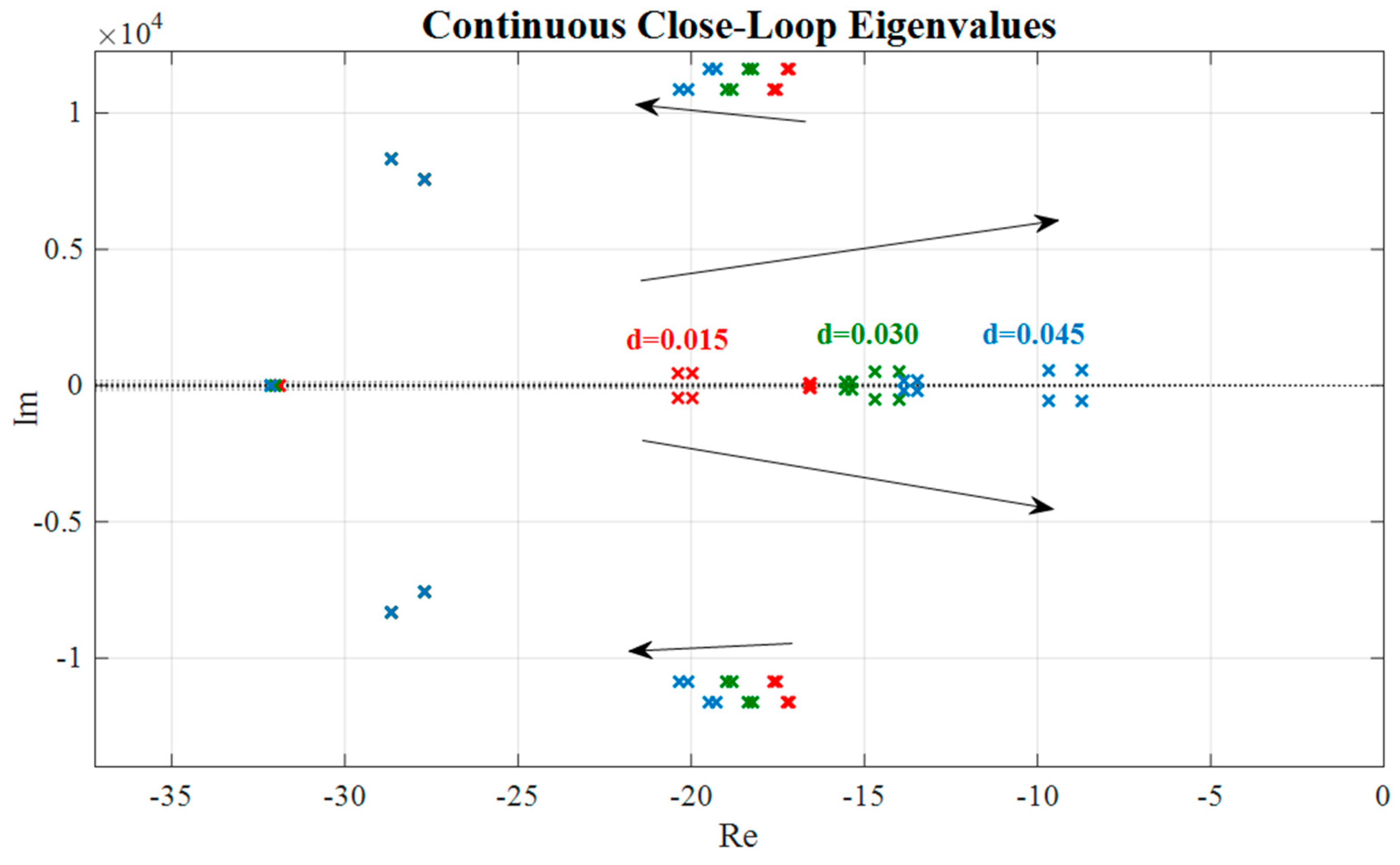
The closed-loop microgrid model (51) can now be used for analyzing the eigenvalue location and step response of an islanded microgrid using the PQ/Vdq droop–boost controller. The open-loop model can be used to analyze the singular value plot of the controlled microgrid to analyze the frequency response under disturbances.

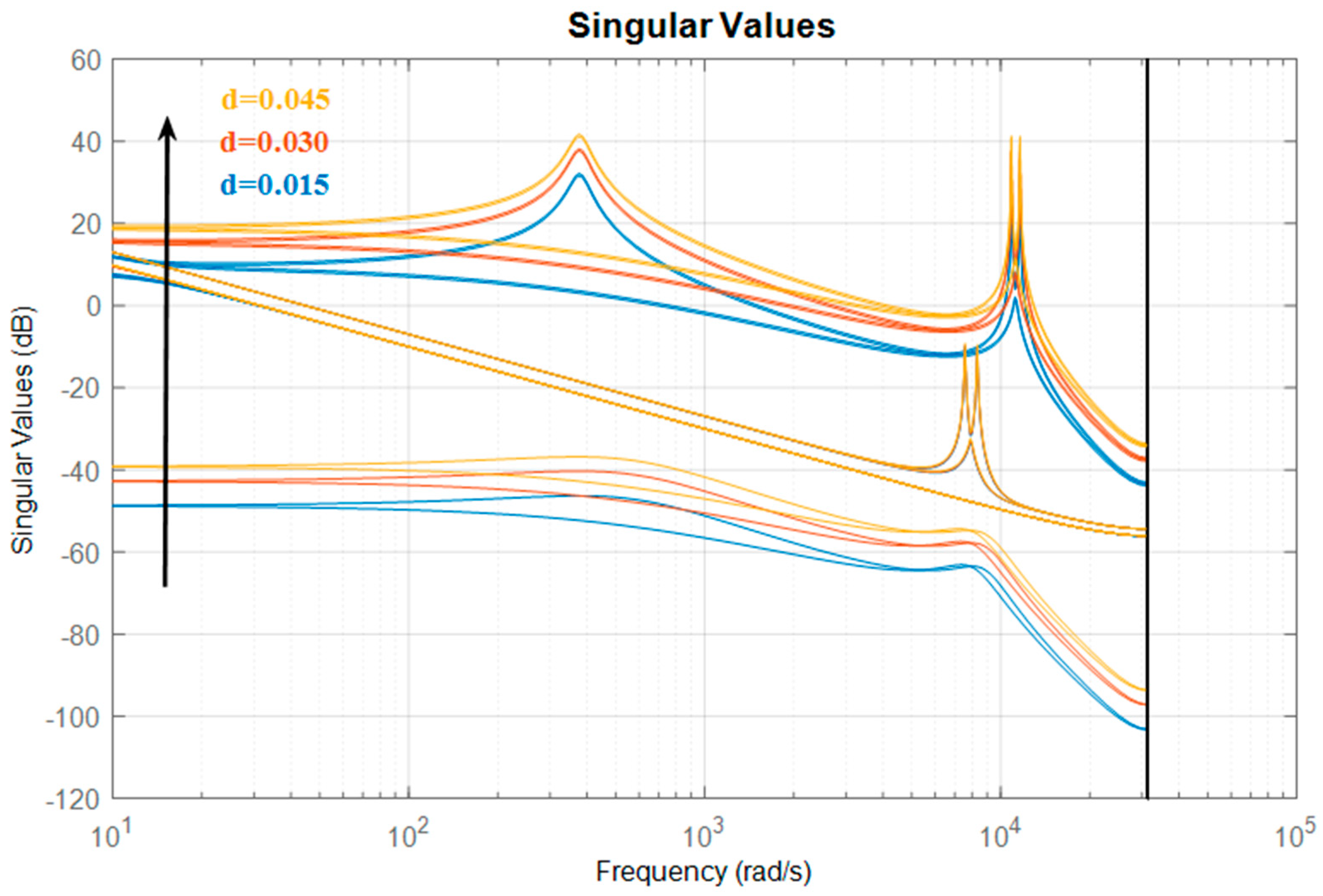
For this experiment, the three inverters have the same rated power. However, for visualization purposes, the droop matrix relation was initially defined as D₂ = 0.9D₁, and D₃ = 0.95D₁. The droop matrix for Inverter 1 was defined as ${\mathrm{D}}_1=\mathrm{d}\left[\begin{array}{cc}1& 0\\ 0& -1\end{array}\right]$. The closed-loop eigenvalues for the islanded microgrid for different values of d are shown in Figure 24. As d increases, the closed-loop eigenvalues tend to the right half plane indicating instability.

To analyze the transient response and frequency response, the singular value diagram is shown in Figure 25. It can be noticed that as d increases, the bandwidth of the open-loop response increases, which makes the system more susceptible to process noise. After analyzing the performance using the three different methods, the droop gains shown in

Table 3. Selected droop gains.

Parameter	m	n
Inverter 1 (D1)	0.028	0.03
Inverter 2 (D2)	0.032	0.032
Inverter 3 (D3)	0.033	0.031

were selected:

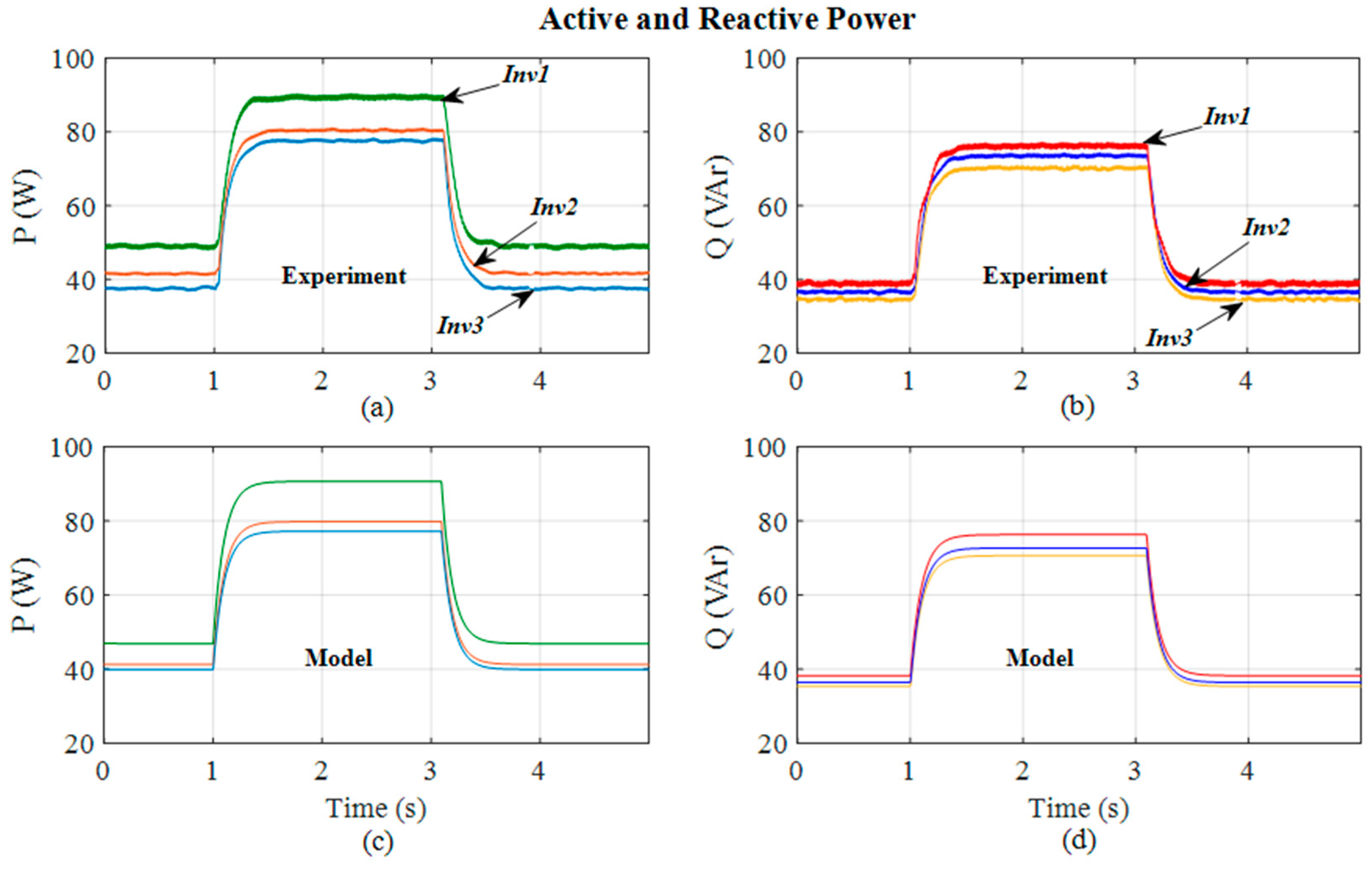
3.3.4. Experimental Results

To assess the performance of the proposed model and to validate the closed-loop model, the experimental setup from Figure 4 was used. The experimental response was compared against the mathematical response of the closed-loop model under load changes. Step changes were analyzed in the mathematical model by generating two different closed-loop models (one for each total load value). Then, when Load 2 was connected in the experiment, that signal swapped the mathematical model and the state of the Load 1 mathematical model became the initial state of the mathematical model for Load 2. Experimental results for this experiment are presented in Figure 26.

It can be seen that although the power responses have slight discrepancies, the dynamic response is similar between the experiment and the mathematical simulation. These discrepancies are generated by deviations on the LCL components and the loads. Results from this experiment demonstrate the effectiveness of the proposed controller and the accuracy of the proposed model.

4. Discussion

In this work, a synchronous model for grid-connected and islanded microgrids is presented. Both models were tested and validated in an experimental setup to demonstrate their accuracy in describing microgrid dynamics. In addition, three scenarios were presented: non-controlled model, LQI power control, and PQ/Vdq droop–boost controller. Both controllers allow to perform stability and performance analysis methods which, unlike approaches found in the literature, can provide a wider perspective of the microgrid in islanded and grid-connected modes. Furthermore, the controlled open-loop model can be used to analyze the microgrid frequency response under disturbances in the process and noise in the sensors. Most of the approaches found in the literature develop the microgrid model based on the controller dynamics, which does not allow to perform open-loop analysis such as singular value diagrams or obtaining stability margins.

The limitations of the proposed models are based on the fact that these models do not include frequency dynamics as other approaches found in literature do. The frequency of the microgrid is assumed static and all inverters are assumed to be synchronized with the common AC bus. Thus, no frequency stability analysis can be performed for the islanded microgrid model. To perform this, the models must include linearized frequency dynamics and their effects on the reactive components of the microgrid. This is seen as a future research direction of this work. Moreover, the mathematical models assume small deviations from the operating point in the AC bus and do not consider certain non-linear dynamics such as transistor switching, DC bus saturation, nor unbalances. Thus, results may have a slight deviation for transient analysis.

The controllers developed in this work are different from the classical droop controller, where the frequency is reduced with the increase in active power and the amplitude is reduced with the reactive power. This implies that frequency does not have considerable distortion, preserving microgrid power quality. In addition, most of the control computations are linear, which allows to perform a stability analysis for state-space controllers. The power is assumed to be linear as the voltage in the AC bus must be close to the nominal values according to power authority regulations. However, further analysis must be done in order to integrate the proposed controllers with synchronous machines or inverters with classical droop controllers, which consider frequency dynamics.

It is important to remark that the proposed models and the application scenarios are intended to be a tool that help readers to implement non-classical power controllers and analyze their stability, robustness, frequency response, and dynamic response. In addition, the proposed models allow readers to implement linear modern controllers that rely on numerical methods such as LQR, Kalman filters, robust controllers and model predictive control. Furthermore, as the model includes the dynamics of power, it could be used to compute optimal control gains for the PQ-Vdq droop–boost controller. This could increase the robustness and stability of the islanded microgrid.

Finally, the methods presented to develop the proposed models can be used in similar approaches to extend the application scenarios to more complex scenarios where other types of generators are integrated. However, special considerations must be done to include the frequency dynamics in the mathematical model.