Effects of the Circuit Arrangement on the Thermal Performance of Double U-Tube Ground Heat Exchangers

Abstract

Given that the issue of variations in geometrical parameters of the borehole heat exchanger (BHE) revolves around the phenomenon of thermal resistance, a thorough understanding of these parameters is beneficial in enhancing thermal performance of BHEs. The present study seeks to identify relative changes in the thermal performance of double U-tube BHEs triggered by alterations in circuit arrangements, as well as the shank spacing and the borehole length. The thermal performance of double U-tube BHEs with different configurations is comprehensively analyzed through a 3D transient numerical code developed by means of the finite element method. The sensitivity of each circuit configuration in terms of the thermal performance to variations of the borehole length and shank spacing is investigated. The impact of the thermal interference between flowing legs, namely thermal short-circuiting, on parameters affecting the borehole thermal resistance is addressed. Furthermore, the energy exchange characteristics for different circuit configurations are quantified by introducing the thermal effectiveness coefficient. The results indicate that the borehole length is more influential than shank spacing in increasing the discrepancy between thermal performances of different circuit configurations. It is shown that deviation of the averaged-over-the-depth mean fluid temperature from the arithmetic mean of the inlet and outlet temperatures is more critical for lower shank spacings and higher borehole lengths.

1. Introduction

In recent years, exploitation of the geothermal energy as a renewable source has witnessed a rapid growth. Geothermal energy, although existing for many years, has gained further recognition recently due to energy shortages [1]. The direct utilization of geothermal energy in conjunction with ground-source heat pumps (GSHPs) has shown great potential for the buildings climatization and domestic hot water (DHW) production. The annual utilization of thermal energy harvested by GSHPs increased by about 40% from 2010 to 2015, with an annual growth rate of 7% [2]. GSHPs are eco-friendly and economically advantageous systems compared to traditional heating systems [3]. The development of GSHP systems can remarkably reduce the primary energy consumption and the emission of greenhouse gases from fossil-based fuels [4].

Ground-coupled heat pumps (GCHPs) emerge as a promising type of GSHPs, because they can be installed in any ground, even where extraction of the groundwater is not allowed. A GCHP system consists of a vertical or horizontal ground heat exchanger, a heat pump, and a distribution system. GCHP systems usually use buried vertical heat exchangers, also called borehole heat exchangers (BHEs). A BHE is generally composed of a single or double high-density polyethylene (HDPE) tube(s) installed in a drilled hole, which is then filled with backfilling materials. The most common BHEs have a diameter of about 15 cm, with lengths ranging between 40 and 200 m. The performance of GCHP systems has been exhaustively investigated by both simulation tools and experiments [5,6,7,8,9,10].

In general, GCHP systems employing the vertical BHEs have higher coefficients of performance (COP). Moreover, they require less ground area due to lower seasonal variations in mean temperature of the ground [11,12]. Despite the advantages of such systems, the central limitations to employing them are their high set-up expenses and drilling costs [13,14,15]. Indeed, a significant portion of the capital cost of GCHPs is attributed to BHEs. A cost sensibility analysis showed that the depth and number of BHEs are the most important parameters to diminish the total cost of GCHP systems [16]. Another study carried out by Blum et al. [17] revealed that the installation cost of a borehole in Germany is 40–50 €/m of the BHE depth, whereas the drilling expenses accounted for a half of this price. In fact, better thermal performance of the BHE results in a lower total required BHE length, and as a consequence a lower total cost.

In the literature, several procedures for the design of BHE fields have been proposed [18,19,20,21]. All methods require knowledge of the thermal conductivity and thermal diffusivity of the ground, the undisturbed ground temperature, and the borehole thermal resistance per unit length [22]. According to ASHRAE [21], the ground thermal conductivity and the borehole thermal resistance are key factors for the design of the BHE size. While the thermal conductivity is a thermophysical property of the ground surrounding the boreholes, the BHE thermal resistance is dependent on the thermal properties of the BHE components, including the U-tube(s) and backfilling materials, the arrangement of the U-tube(s), and the operational parameters [23]. A comprehensive understanding of these parameters is, therefore, essential in enhancing the efficiency of GCHP systems.

The borehole thermal resistance is a critical design parameter and a key performance characteristic of a BHE [24,25]. The lower thermal resistance leads to the better thermal performance of the BHE and to the lower total required BHE length. Several innovative designs have been recently proposed in order to diminish the borehole thermal resistance and to improve the thermal performance of GCHPs, including thermally-enhanced circuiting fluid, pipes, and backfilling materials, as well as various novel configurations of BHEs [26,27,28,29,30,31].

Double U-tube boreholes are the second most employed kind of BHE after single U-tube BHEs. The double U-tube configuration gives lower borehole thermal resistance values than the single U-tube configuration, since it has a larger heat transfer area between the circuiting fluid and the surrounding ground. Nonetheless, it requires more piping materials and consumes more pumping power for a certain demand. In particular, two U-tubes inside a double U-tube BHE can be connected in either a parallel circuit or in series circuit. Previous studies confirmed that the double U-tube BHE parallel configuration provides better thermal performance than the double U-tube BHE series configuration [32,33].

Recently, several studies have been conducted on the performance and optimization of double U-tube BHEs. For instance, Zhu et al. [34] numerically studied the thermal performance of a double U-tube BHE by means of a transient heat transfer model. The impacts of various operational parameters were analyzed, such as the inlet velocity and operation interval on the axial and radial ground temperature distribution. The numerical results indicated that the increased amplitude of the BHE’s heat transfer rate was similar when the charging temperature was increased under the same velocity conditions. Quaggiotto et al. [35] investigated the thermal comportment of double U-tube BHEs and compared their performance to coaxial BHEs by means of a series of numerical simulations. The analysis took into account two different ground types, with different the thermal conductivity values. The results showed that the ground with the higher value of the thermal conductivity highlights the higher output of the coaxial probe.

By means of the Taguchi method and utility concept, Kumar and Murugesan [36] carried out a study on the optimization of the geothermal interaction of a double U-tube BHE for heating and cooling applications. The main goal of the optimization was to obtain maximum heat rejection during space cooling and maximum heat extraction during space heating operations. In another study, Kerme and Fung [37] proposed a numerical model to predict the transient heat transfer in double U-tube BHEs, where the U-tubes could operate with either different or equal inlet fluid temperatures and mass flow rates.

Most of the recent numerical analyses on the performance of double U-tube BHEs have focused on the influence of thermophysical and operational parameters, such as the ground and grout thermal conductivity, inlet fluid temperature, and volume flow rate. However, fewer attempts have been made to identify the performance sensitivity of double U-tube BHEs on variation of the geometrical parameters, particularly the circuit arrangements. In fact, the arrangement of flow channels and the shank spacing, namely the center-to-center distance between opposite pipes, are geometrical parameters that significantly affect the thermal performance of a BHE. Given that the issue of variations in the aforementioned parameters revolves around the phenomenon of thermal short-circuiting and borehole thermal resistance, a comprehensive investigation of these parameters is beneficial in enhancing the thermal performance of BHEs.

The present study seeks to analyze associated changes in the thermal performance of a double U-tube BHE connected in parallel circuit, triggered by variations in the outlined parameters, namely the circuit arrangement and shank spacing, as well as the borehole length. A comprehensive numerical analysis is carried out by applying a 3D transient finite element code implemented in COMSOL Multiphysics. The borehole thermal resistance and the temperature difference between the system inlet and outlet are treated as critical parameters to evaluate the thermal performance of the BHE. Since the latter is directly related to the COP of a GCHP system, its relative changes in each configuration are assessed for different shank spacing and borehole length values. The impact of the thermal interference between flowing legs, namely the thermal short-circuiting effect, on parameters affecting the borehole thermal performance is addressed. Furthermore, the thermal effectiveness of the double U-tube BHEs with various circuit configurations is evaluated via the effectiveness coefficient for different shank spacings and borehole lengths.

2. Methodology

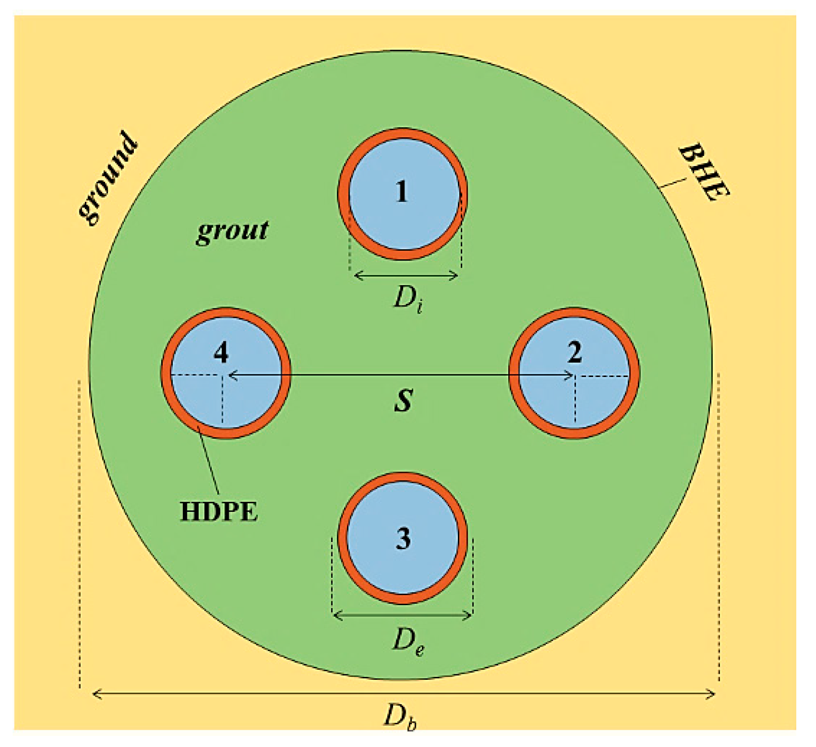
The case under study is a double U-tube BHE surrounded by the ground, composed of HDPE U-pipes sealed with the grout. A customary BHE with diameter D_b = 152 mm was considered, with U-tubes having an internal diameter D_i = 26 mm and external diameter D_e = 32 mm. The ground surrounding the BHE was modeled as a cylinder coaxial with the borehole, having a diameter equal to 10 m and a length 10 m longer than the BHE. The model of the BHE lower section was simplified by eliminating the U-junction at the bottom of the U-loop. It is well-known that the removal of a U-shaped connector has no considerable effect on the obtained results and that it significantly reduces the computational cost [38]. Various values for the shank spacing were selected, ranging from 65 mm to 105 mm. In addition, four different borehole lengths were considered, namely 50, 100, 150. and 200 m. A sketch of the borehole cross-section is illustrated in Figure 1.

Indeed, for two U-tubes connected in a parallel circuit inside the BHE, various combinations of circuit arrangements come down to two choices that are influential in the heat transfer process between the borehole and the ground, represented by notations (1-2,3-4) and (1-3,2-4). These four digits indicate the number of the tubes, as shown in Figure 1. Here, (1-2,3-4) implies that the fluid flows through pipes 1 (inlet) and 2 (outlet), and also through pipes 3 (inlet) and 4 (outlet). A quasi-3D analytical model for BHE heat transfer developed by Zeng et al. [32] showed that a double U-tube BHE with (1-2,4-3) configuration is of the same nature as one with (1-3,2-4) configuration. However, for a double U-tube BHE with two independent circuits, the (1-2,4-3) configuration may be considered a distinct circuit arrangement [33]. In the present study, the thermal performances of three configurations are separately evaluated. We will show that for the symmetric disposal of the tubes and equivalent mass flow rates, the thermal resistance and temperature profiles of these configurations, namely (1-3,2-4) and (1-2,4-3), can be considered as almost identical.

The computational domain consists of three solid domains, namely the HDPE pipes, grout, and ground, along with a fluid domain inside the U-loops. The values of the thermophysical properties adopted for solid materials are reported in

Table 1. Thermophysical properties of solids materials.

Title	Unit	Ground	Grout	HDPE
Heat capacity per unit volume	MJ m−3 K−1	2.5	1.6	1.824
Thermal conductivity	W m−1 K−1	2.2	1.8	0.5

.

The summer-cooling operation was examined, with the inlet fluid temperature equal to T_in = 32 °C. Water was considered as the working fluid, flowing with uniform velocity in the vertical direction. The model took into account only the energy balance equation through the fluid domain. The boundary condition of the third kind, i.e., convective heat transfer, was imposed at the fluid–solid interface. Equality of boundary heat fluxes and temperature was applied as a coupling condition. Furthermore, temperature continuity was assumed between the pipes and the grouting material, and between the BHE and the ground. Values of the fluid thermal properties; the volume flow rate; the heat transfer coefficient h; and the Reynolds, Nusselt, and Prandtl numbers are reported in

Table 2. Thermophysical properties of the fluid and thermohydraulic characteristics of the flow.

ρ	cp	k	μ	V	h	Re	Nu	Pr
[kg m−3]	[J kg−1 K−1]	[W m−1 K−1]	[mPa s]	[dm3 min−1]	[W m−2 K−1]
995.03	4179.5	0.6187	0.7646	14	1436.4	7435	60.36	5.165

.

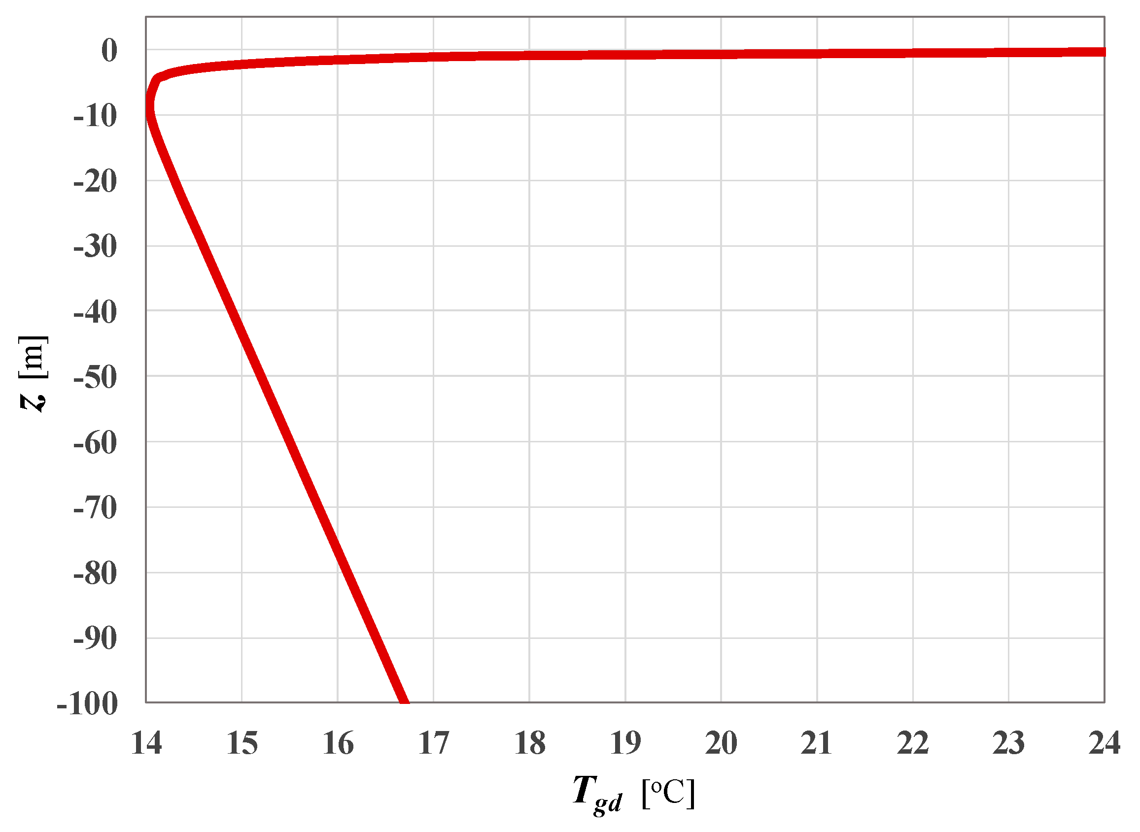
As a boundary condition, the surface at z = 0 of the BHE, namely the ground level, was considered as adiabatic, whereas that of the ground was assumed to be isothermal, with T_gd (0) = 24 °C. At the external boundary of the computational domain, the bottom and lateral surfaces of the ground were considered as adiabatic. The initial temperature of the ground and of the BHE was set equal to the undisturbed ground temperature. It was supposed that the undisturbed ground temperature, T_gd, was equal to 14 °C at depth z = 10 m, with geothermal gradient 0.03 °C per meter for z > 10 m. For z < 10 m, an exponential variation of the ground temperature with depth was considered. The following distribution of T_gd (z) was assumed [39]:

$$\{\begin{array}{cc}{T}_{gd}\left(z\right)=T_{gd}\left(10\right)+\left[T_{gd}\left(0\right)-T_{gd}\left(10\right)\right]\times e^{-z}\hfill & 0\le z\le 10\mathrm{m}\\ T_{gd}\left(z\right)=14+0.03\times z\hfill & z>10\mathrm{m}\end{array}$$

(1)

The mean value of the T_gd between 0 and 100 m and between 0 and 200 m turned out to be 15.31 °C and 16.75 °C, respectively. Figure 2 demonstrates the profile of T_gd between 0 and 100 m.

The general energy balance equations for solid and fluid domains can be given as:

$${\left(\rho c\right)}_i\frac{\partial T}{\partial t}=k_{i,x}\frac{{\partial }^{2}T}{\partial x^2}+k_{i,y}\frac{{\partial }^{2}T}{\partial y^2}+k_{i,z}\frac{{\partial }^{2}T}{\partial z^2}$$

(2)

$${\rho }_f{c}_{p,f}\left(\frac{\partial T}{\partial t}+u\frac{\partial T}{\partial z}\right)=k_{f,x}\frac{{\partial }^{2}T}{\partial x^2}+k_{f,y}\frac{{\partial }^{2}T}{\partial y^2}+k_{f,z}\frac{{\partial }^{2}T}{\partial z^2}$$

(3)

where the subscript i refers to properties of the i-th solid (HDPE pipes, grout, and ground) and the subscript f refers to properties of the fluid.

A rescaling method was worked out in order to have a more compact shape of the computational domain. The vertical coordinate z was replaced by a reduced one, $\tilde{z}=z/\gamma$, and anisotropic thermal conductivity was applied for both solid and fluid domains. While reduced thermal conductivity ${\tilde{k}}_z=k_z/{\gamma }^2$ was considered along the vertical direction, the real thermal conductivity was imposed in the horizontal directions, namely k_x and k_y. In addition, for the velocity term in the vertical direction, reduced fluid velocity was considered, namely $\tilde{u}=u/\gamma$. If one replaces the transformation explained above, Equations (2) and (3) take the following form:

For each pair of corresponding values of $z$ and $\tilde{z}$, it can be verified that Equations (2) and (3) can be considered as identical to Equations (4) and (5). For BHEs with lengths of 50, 100, 150, and 200 m, the reduction coefficient γ was set equal to 5, 10, 15, and 20, respectively.

$${\left(\rho c\right)}_i\frac{\partial T}{\partial t}=k_{i,x}\frac{{\partial }^{2}T}{\partial x^2}+k_{i,y}\frac{{\partial }^{2}T}{\partial y^2}+{\tilde{k}}_{i,z}\frac{{\partial }^{2}T}{\partial {\tilde{z}}^2}$$

(4)

$${\rho }_f{c}_{p,f}\left(\frac{\partial T}{\partial t}+\tilde{u}\frac{\partial T}{\partial \tilde{z}}\right)=k_{f,x}\frac{{\partial }^{2}T}{\partial x^2}+k_{f,y}\frac{{\partial }^{2}T}{\partial y^2}+{\tilde{k}}_{f,z}\frac{{\partial }^{2}T}{\partial {\tilde{z}}^2}$$

(5)

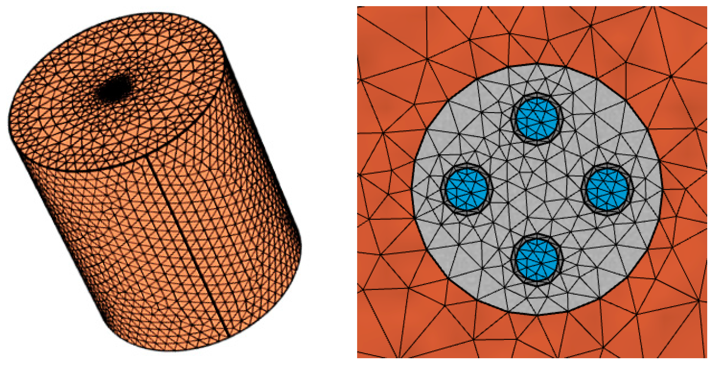
A 3D transient finite element code, implemented through COMSOL Multiphysics, was developed to solve the conjugate heat transfer problem for a working period of 100 h. The selected operation period is adequate to reach a steady-flux regime. The time-dependent “PARDISO” solver with non-uniform time steps was employed to solve the transient heat transfer problem. Values of the relative and absolute tolerance were set equal to 10⁻³ and 10⁻⁴, instead of the default values, to improve the precision of simulations. The unstructured tetrahedral grid was utilized to mesh the computational domain. The selected mesh for final computations, shown in Figure 3, contains approximately 1.6 × 10⁶ tetrahedral elements, varying to some extent with the BHE configuration.

3. Model Validation

To ensure that the results obtained by the numerical simulations were mesh-independent, a series of preliminary simulations with different meshes were performed. A mesh independence check was carried out for a case with the (1-2,3-4) arrangement, L = 100 m, S = 85 mm, and the thermohydraulic characteristics reported in Table 2. Values of the outlet fluid temperature, T_out, obtained by different meshes at t = 20 h and their corresponding percentage deviations from mesh 3 (i.e., the mesh employed for final computations) are presented in

Table 3. Mesh independence check.

Mesh	Elements	Tout [°C]	Deviation from Mesh 3 [%]
1	1,361,246	25.124	0.05
2	1,492,251	25.127	0.04
3	1,586,586	25.136	-
4	1,656,432	25.131	0.02
5	1,790,728	25.125	0.04

. It is evident that the results obtained by various grids are almost coincident, with a maximum absolute percent deviation equal to 0.05%.

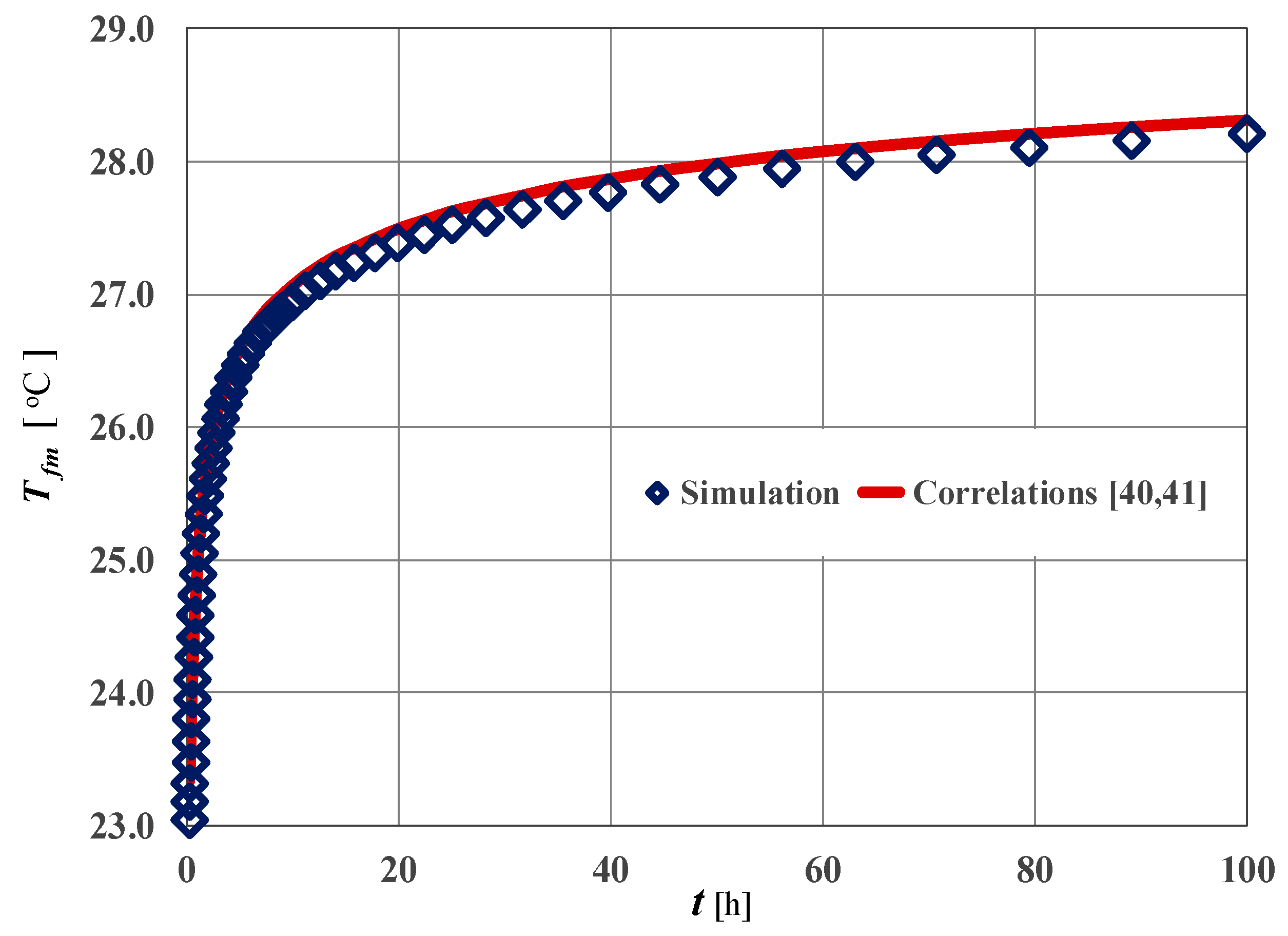
In order to validate the employed numerical code, the time evolutions of the mean fluid temperature, T_f,m, obtained through simulations, were compared with those determined by applying the correlations proposed in [40,41]. These correlations were deduced to evaluate T_f,m by linear regression of a dimensionless coefficient with the best fitting method. The selected case for the model validation has a circuit arrangement of (1-3,2-4), L = 100 m, and S = 85 mm, simulated for the operation time interval ranging from 0 to 100 h.

Figure 4 shows plots of T_f,m versus time, obtained by simulations and by applying the correlations. The figure shows a fair agreement between numerical results and those obtained through correlations. The mean square deviation (MSD) of the results obtained numerically from those obtained through the correlations can be determined by:

$$MSD=\sqrt{\frac{{\displaystyle {\sum }_{i=1}^N{\left({\left[{\phi }_{Num}\right]}_i-{\left[{\phi }_{Corr}\right]}_i\right)}^2}}{N}}$$

(6)

where ϕ is an arbitrary parameter. The MSD of the mean fluid temperature, T_f,m, obtained by numerical simulation from T_f,m obtained through the correlations is 0.29 °C, equal to a normalized MSD of 1.05%.

Additional validation of the numerical model was carried out by making a comparison between values of the 3D borehole thermal resistance, R_b-3D, evaluated through numerical simulations, and those calculated by an analytical equation developed by Conti et al. [42] through the line-source model, denoted as R_b-C. Values of the R_b-3D and R_b-C were calculated through Equations (7) and (8):

$$R_{b-3D}=\frac{T_{f,m}-T_{b,m}}{q_l}$$

(7)

$$R_{b-C}=\frac{1}{8\pi k_{gt}}\left[\ln \left(\frac{D_b}{D_e}\right)+2\ln \left(\frac{D_b}{\sqrt{2}S/2}\right)+\ln \left(\frac{D_b}{S}\right)-\frac{k_{gt}-k_{gd}}{k_{gt}+k_{gd}}\left(\frac{D_b^8-{(S/2)}^8}{D_b^8}\right)\right]+\frac{R_p}{4}$$

(8)

where in Equation (7), T_f,m is the mean fluid temperature determined by integral of fluid temperature over the BHE length, T_b,m is the mean BHE surface temperature, and q_l is the mean heat flux per unit length exchanged between the ground and BHE. In Equation (8), R_p is the thermal resistance of each HDPE pipe, which can be determined by:

$$R_p=\frac{1}{2\pi k_p}\ln \frac{D_e}{D_i}+\frac{1}{h\pi D_i}$$

(9)

Table 4. Comparison of the borehole thermal resistance evaluated by numerical simulation and that determined through the analytical model [42].

S [mm]	Rb-3D [W−1 mk]	Rb-C [W−1 mk]	Discrepancy [%]
65	0.0786	0.0788	0.27
85	0.0612	0.0610	0.32
105	0.0467	0.0469	0.43

compares values of R_b-3D and R_b-C for three different values of the shank spacing. Values of the R_b-3D, evaluated through Equation (7), were obtained numerically as an average of the R_b-3D in the steady-flux regime, namely the time interval ranging between 2 and 100 h. The table shows that the numerical results are in good agreement with those obtained by applying the analytical method. The maximum discrepancy between results is 0.43% for the case with highest shank spacing, namely S = 105 mm.

4. Preliminary Performance Analysis of Different Circuit Arrangements

In the present section, the thermal performance of various circuit arrangements of a double U-tube BHE is analyzed. The results were obtained for configurations having intermediate values for the shank spacing and BHE length, namely S = 85 mm and L = 100 m, respectively.

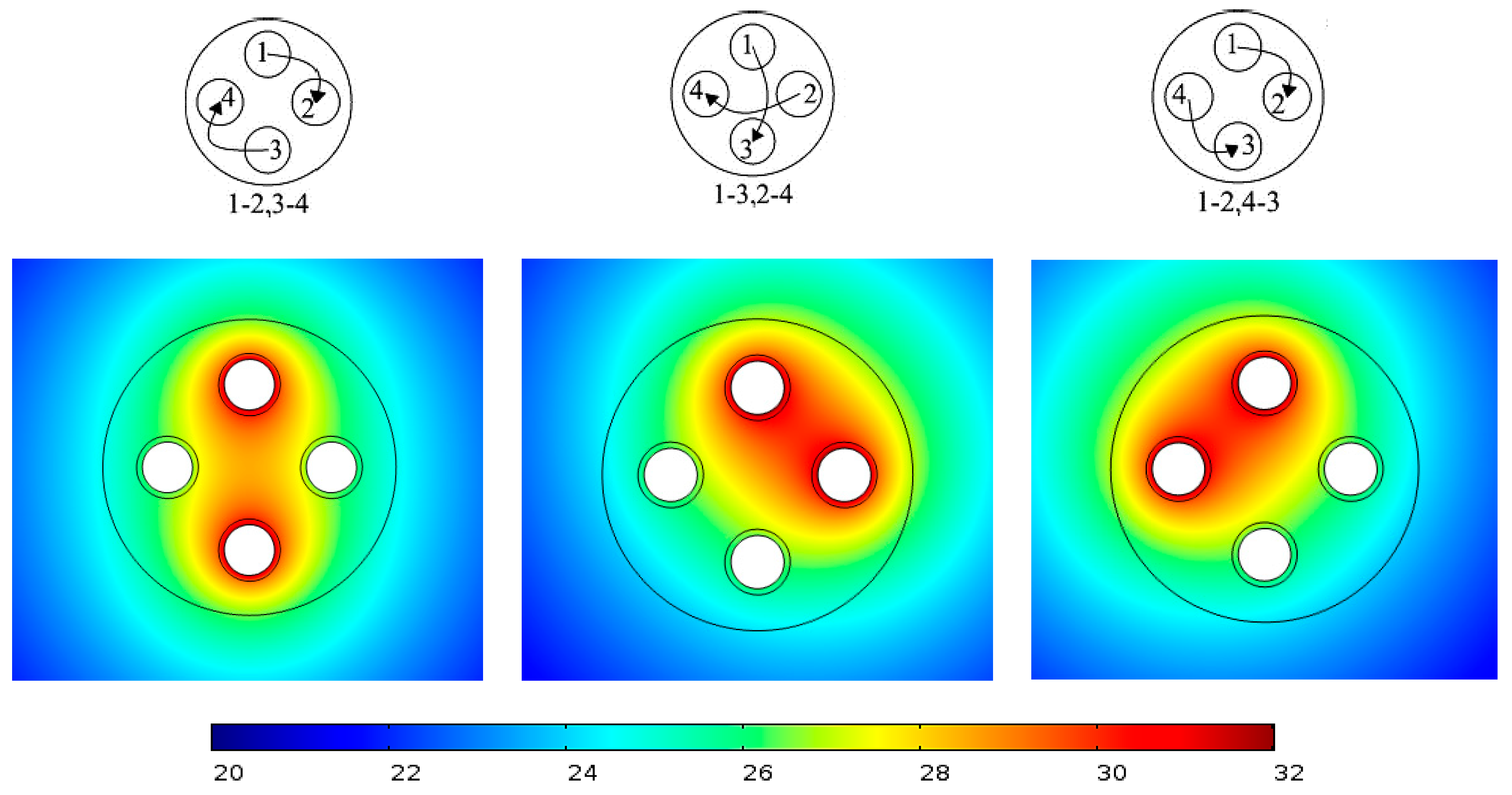
Isothermal contours, presented in Figure 5, display the temperature distribution inside and around the double U-tube BHE with different circuit arrangements, at horizontal surface z = 0 and at t = 100 h. The figure demonstrates that configuration (1-2,3-4) has a distinct temperature distribution; it shows a higher thermal interference between the upward and downward flowing legs, compared with two other configurations, namely (1-3,2-4) and (1-2,4-3). In the following, it will be shown that the higher thermal interference, namely thermal short-circuiting, flowing between legs of such configuration leads to a lower thermal performance in comparison with other configurations.

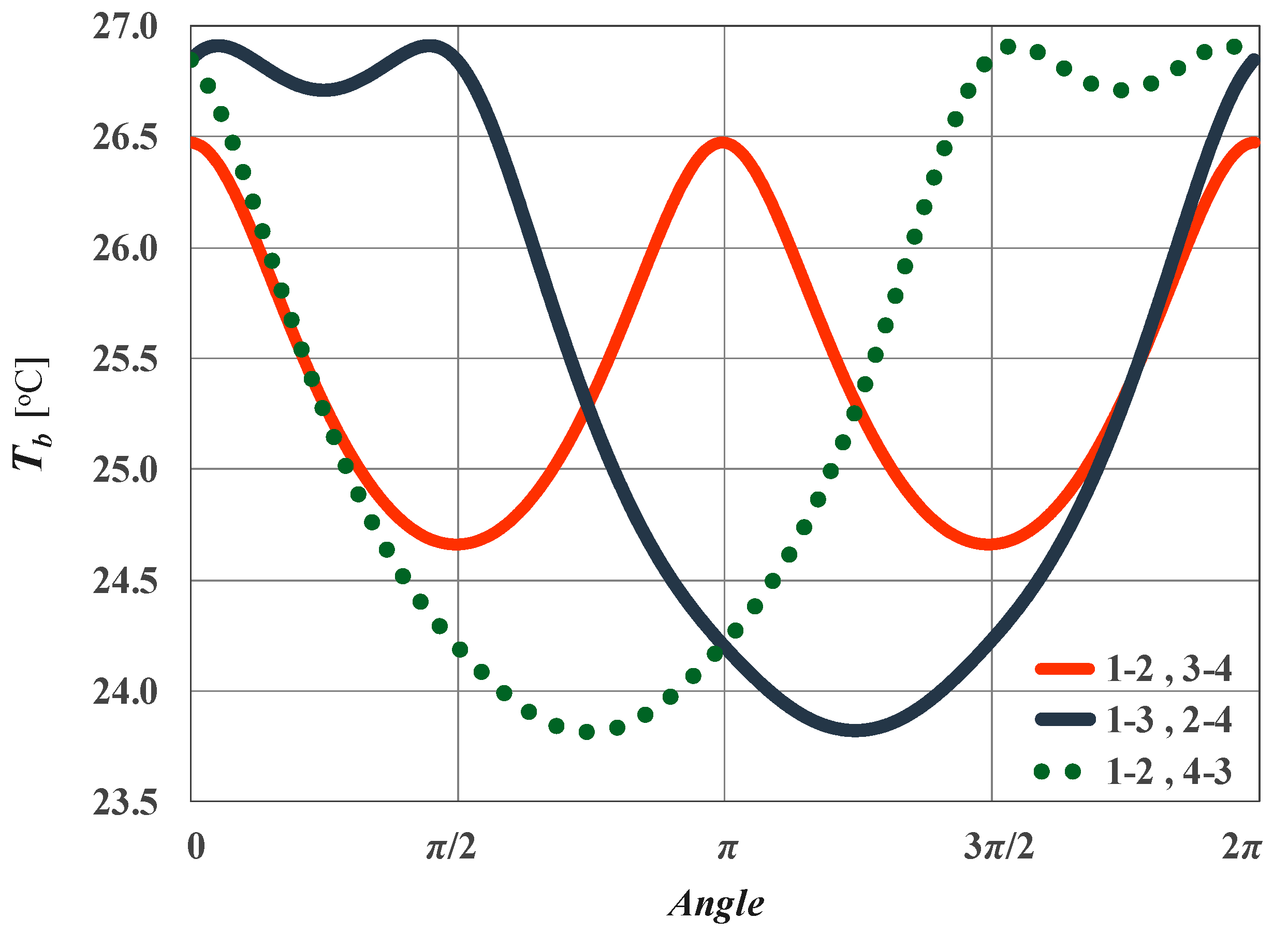
Figure 6 demonstrates the angular temperature distribution along the BHE perimeter, at horizontal surface z = 0 and at t = 100 h. It should be noted that angle 0 refers to the upper point of tube no. 1 in Figure 1. The plots show the non-uniformity of the temperature distribution along the perimeter of the borehole. It is evident that configurations (1-3,2-4) and (1-2,4-3) have a symmetrical temperature distribution along the BHE surface, with identical maximum and minimum temperature values equal to T_b-max = 26.91 °C and T_b-min = 23.82 °C, respectively.

In fact, the borehole thermal resistance per unit length is defined either through 3D thermal resistance definition, as presented in Equation (7), or through effective thermal resistance definition:

$$R_{b-eff}=\frac{T_{f,ave}-T_{b,m}}{q_l}$$

(10)

where T_f,ave is the arithmetic mean of the inlet and outlet fluid temperature. In the present study, both definitions of the BHE thermal resistance have been taken into account. However, corresponding results of the R_b-3D are not presented here for the sake of brevity. Henceforth, the effective thermal resistance is denoted as R_b for simplicity.

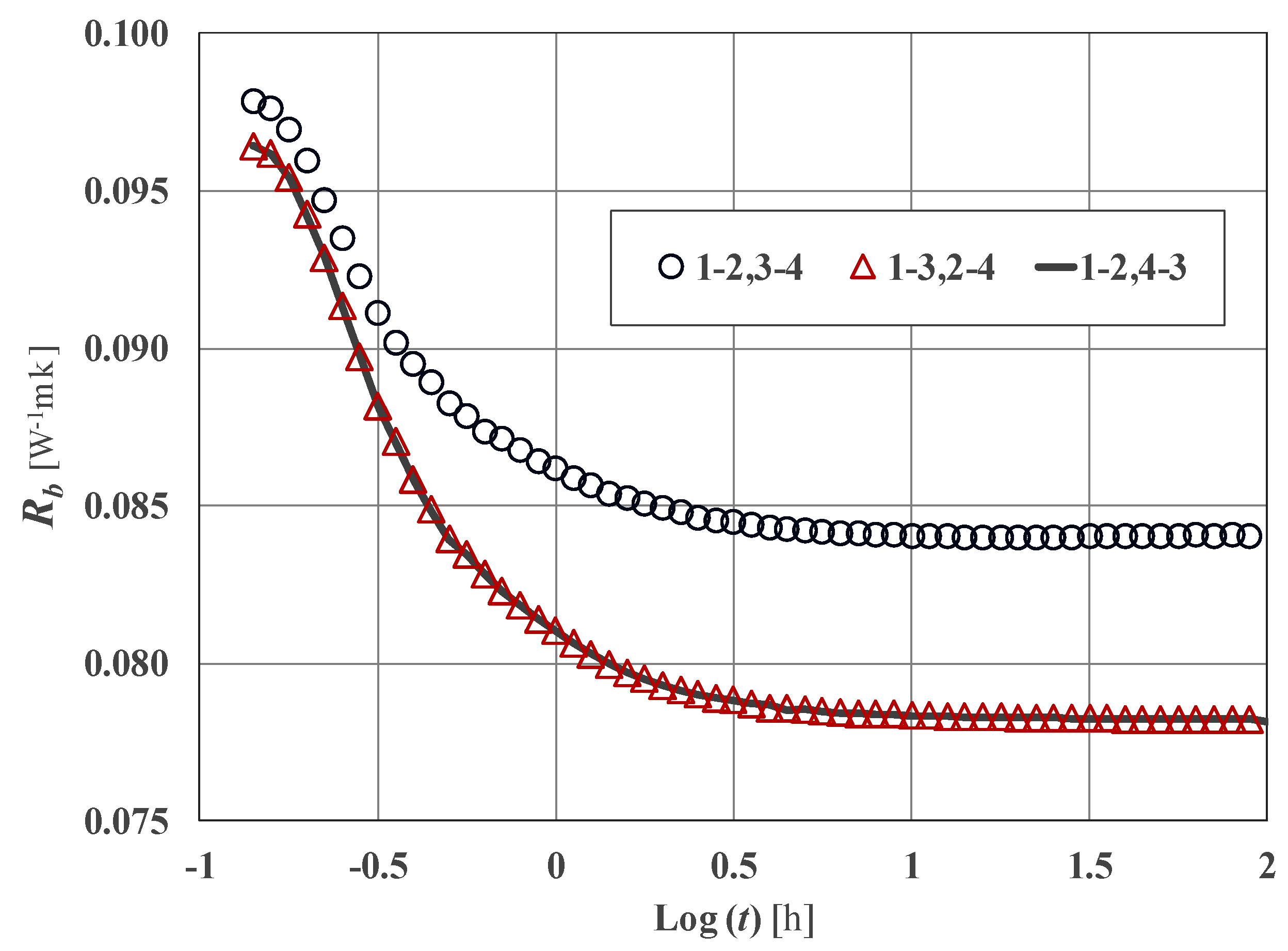
Plots of the borehole thermal resistance, R_b, versus a logarithmic scale of time in hours are presented in Figure 7. The figure shows that plots of R_b reach a time-independent value, particularly after the first 2 h of simulations. The figure demonstrates a significant difference between the thermal resistance of configuration (1-2,3-4) and configuration (1-3,2-4) or (1-2,4-3), with normalized mean square deviation equal to 6.71%. Aside from the very first minutes, the difference between the borehole thermal resistance of configurations (1-3,2-4) and (1-2,4-3) is vanishing; this confirms that for a symmetric disposal of the tubes and equivalent mass flow rates, the thermal performance of these configurations can be considered identical.

For configuration (1-2,3-4), the higher value of the effective thermal resistance (presented in Figure 7) and higher thermal interference between tubes (presented in Figure 5) are evidence of the impact of thermal short-circuiting on the thermal performance of this kind of circuit arrangement.

To highlight this effect, an additional numerical simulation for configuration (1-2,3-4) was performed. Following the same model and conditions, an adiabatic rectangular surface crossing the BHE center with sides equal to the diameter and length of the BHE was inserted in order to cut the thermal interreference between upward and downward flowing legs. The obtained results are reported in

Table 5. Effects of thermal short-circuiting on relevant parameters of thermal performance.

	Arrangement
Parameter	(1-2,3-4)	(1-3,2-4)	(1-2,3-4)ad
(Tin -Tout) [°C] [°C]	5.65	5.76	5.73
Tb,m [°C]	24.78	24.96	24.91
ql [Wm−1]	54.76	55.77	55.60
Rb [W−1 mK]	0.0841	0.0783	0.0784

, denoted as (1-2,3-4)_ad.

The table compares parameters reflecting the BHE thermal performance for different circuit arrangements. It shows the superiority of the configuration (1-3,2-4) in terms of thermal performance in comparison with other configurations. While the results represent the lowest performance for configuration (1-2,3-4), configuration (1-2,3-4) with an adiabatic surface, i.e., (1-2,3-4)_ad, shows similar performance to configuration (1-3,2-4). This indicates that the lower thermal performance of configuration (1-2,3-4) is mainly due to the thermal short-circuiting effect.

5. Variation of Shank Spacing

Shank spacing is a parameter that may affect the BHE thermal resistance, and therefore the thermal performance of U-tube BHEs. The ideal arrangement of the U-tube(s) within the BHE is when the U-tube legs are as close as possible to the wall surface of the BHE. This configuration leads to a lower borehole thermal resistance, independently of the other influential parameters. In this section, the thermal performance sensitivity of two different circuit configurations, namely (1-2,3-4) and (1-3,2-4), to the shank spacing variation is assessed. Five shank spacings were selected, varying from 65 mm (close spacing) to 105 mm (wide spacing). The borehole thermal resistance and outlet fluid temperature were considered as parameters reflecting the thermal performance of the borehole.

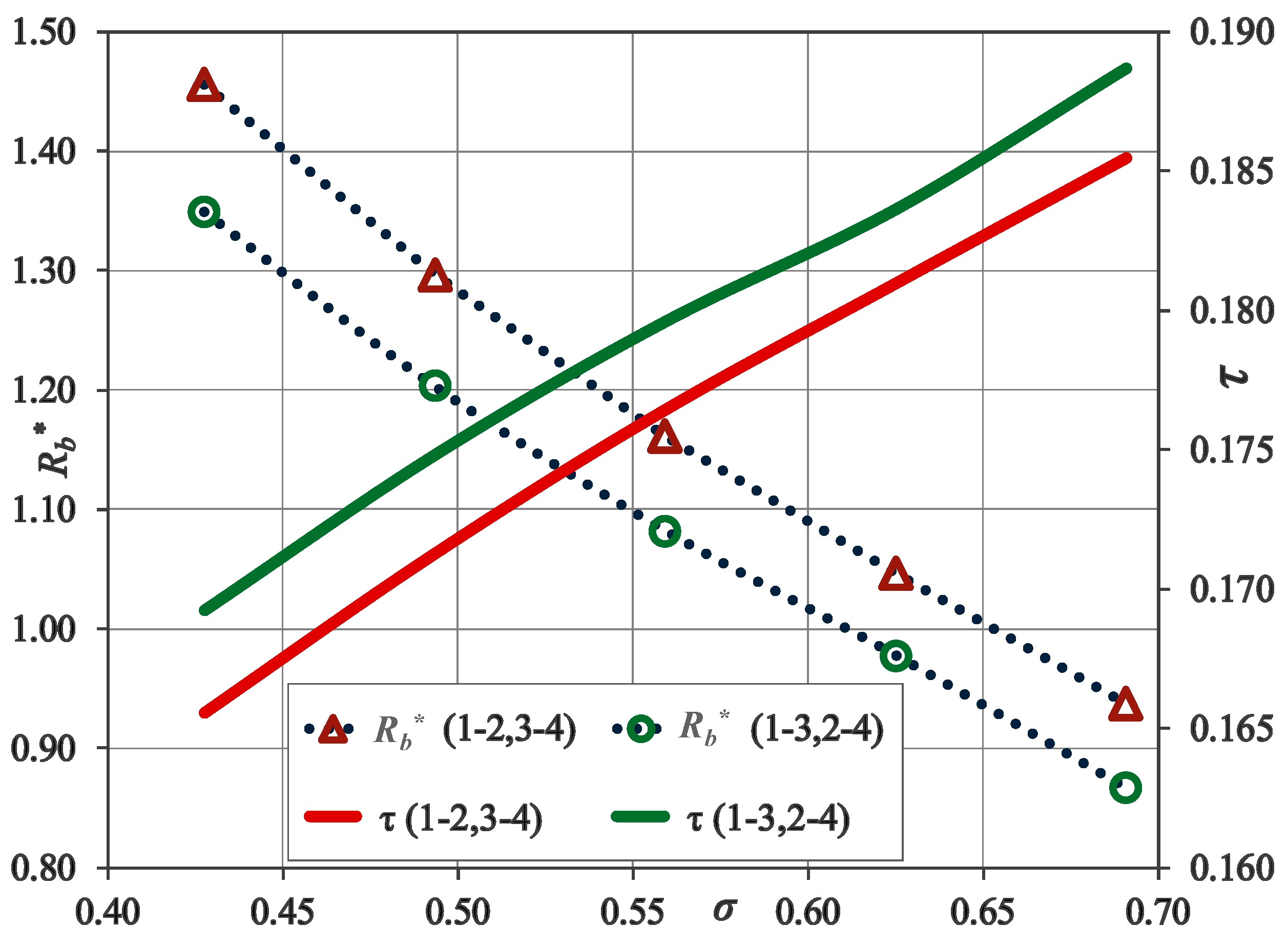
Figure 8 displays the variations of the dimensionless borehole thermal resistance, R_b^*, and dimensionless outlet fluid temperature, τ, versus dimensionless shank spacing, defined as σ = S/ D_b, at t = 100 h. The figure shows that the dimensionless thermal resistance, defined as R_b^* = 2π k_gd R_b, is a decreasing function of the shank spacing; the wider the shank spacing, the lower the BHE thermal resistance. For different shank spacing values, it is evident that configuration (1-3,2-4) has a lower thermal resistance compared with configuration (1-2,3-4), with an average difference of 7.17%.

Plots of the dimensionless parameter τ, defined as (T_in −T_out)/T_in, versus σ show that τ increases almost linearly with shank spacing. Due to a lower thermal resistance, configuration (1-3,2-4) gives higher values of τ, i.e., a lower outlet fluid temperature. The figure demonstrates that the differences between plots of τ decrease to some extent with increasing shank spacing.

The sensitivity of the borehole thermal resistance and outlet fluid temperature to variations of shank spacing is reported in

Table 6. Sensitivity of thermal resistance and outlet fluid temperature to shank spacing variation.

	(1-2,3-4)		(1-3,2-4)
S [mm]	ΔRb [%]	ΔT [%]	ΔRb [%]	ΔT [%]
65	-	-	-	-
75	10.96	3.45	10.82	3.31
85	20.23	6.57	19.77	6.13
95	28.09	9.31	27.52	8.51
105	35.61	12.02	35.76	11.51

for both configurations at t = 100 h. The table presents the decrement percentage of R_b^*, denoted by ΔR_b, and the increment percentage of τ, denoted by ΔT, with respect to the lowest employed value of shank spacing, namely S = 65 mm. As one can expect, values of ΔR_b and ΔT increase with shank spacing for both circuit configurations. However, configuration (1-2,3-4) is more sensitive to shank spacing variation, particularly for lower shank spacing values.

It is also noticeable that configuration (1-2,3-4) shows a slightly better improvement rate for thermal performance with increasing shank spacing compared with configuration (1-3,2-4). This could be due to the weakening effect of thermal short-circuiting with increasing distance between opposite flowing tubes. Moreover, by increasing the shank spacing, the difference between the ΔR_b of configuration (1-2,3-4) and that of configuration (1-3,2-4) is diminished.

The table shows that with a 4 cm increase of the shank spacing, the borehole thermal resistance can decrease more than 35%, while ΔT increases by about 12%. This implies that the borehole thermal resistance is quantitively more sensitive than the outlet fluid temperature to shank spacing variation.

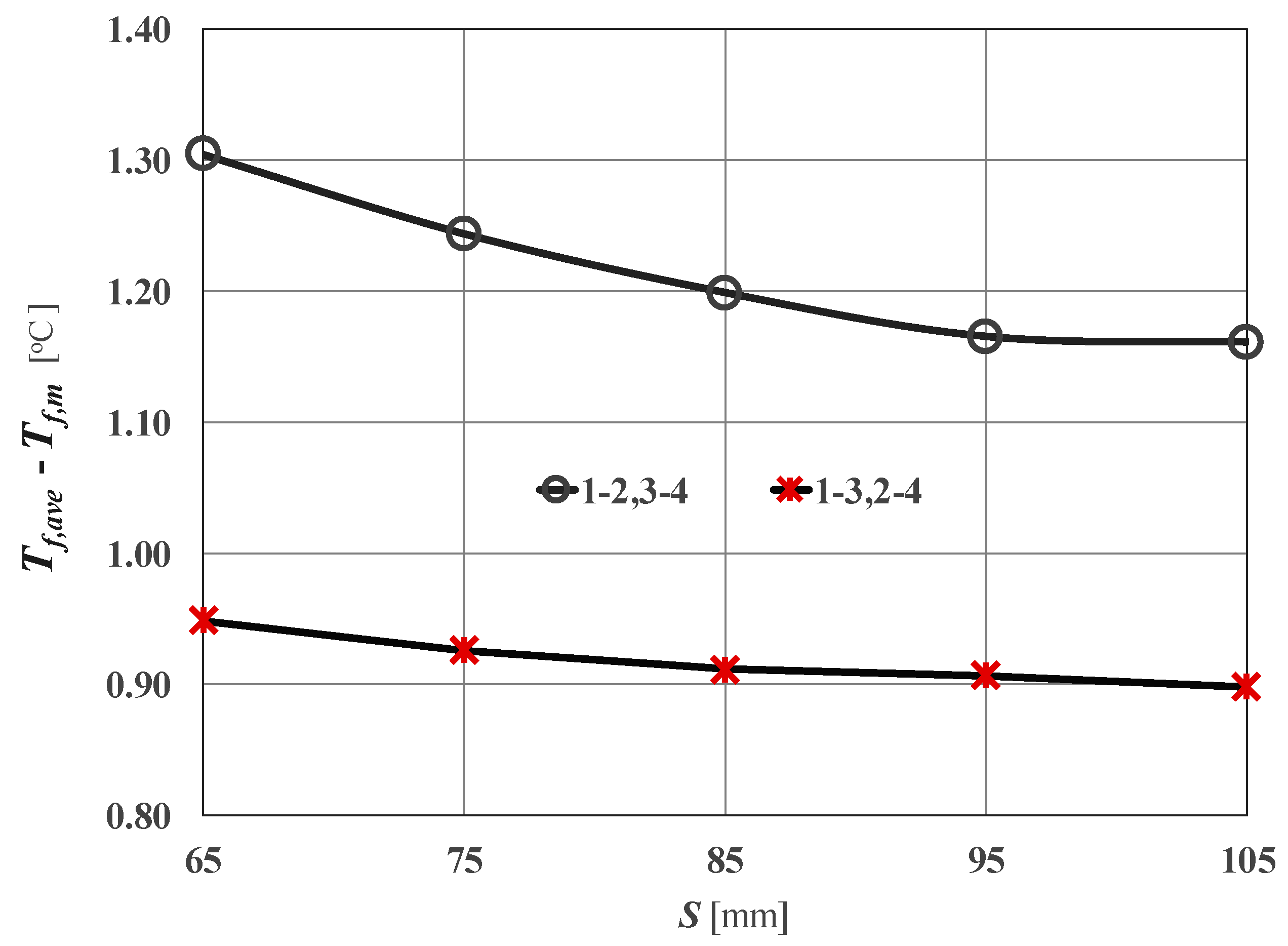
The thermal short-circuiting causes the averaged-over-the-depth mean fluid temperature (T_f,m in Equation (7)) to deviate from the arithmetic mean of the inlet and outlet temperatures, namely the average fluid temperature (T_f,ave in Equation (10)). Figure 9 demonstrates the difference between the mean fluid temperature T_f,m and average fluid temperature T_f,ave for various shank spacing values. The figure shows that the difference between T_f,ave and T_f,m decreases with increasing shank spacing for both circuit configurations. However, the decreasing trend for the plots is not of the same order.

Due to the higher thermal interreference between tubes in configuration (1-2,3-4), the decrease of (T_f,ave − T_f,m) with shank spacing is significant, in particular for lower shank spacing values. On the other hand, in configuration (1-3,2-4), the dependence of (T_f,ave − T_f,m) on shank spacing is marginal. Nevertheless, even for the widest shank spacing, it can be observed that a 0.27 °C difference between plots of configurations (1-2,3-4) and (1-3,2-4) remains. In the next section, we will show that the borehole length has an even more severe impact on this difference.

6. Effects of the Borehole Length

In order to investigate the impact of the borehole length on the thermal performance of different configurations under study, various borehole lengths were considered, ranging from 50 to 200 m, each with an intermediate shank spacing value, i.e., S = 85 mm.

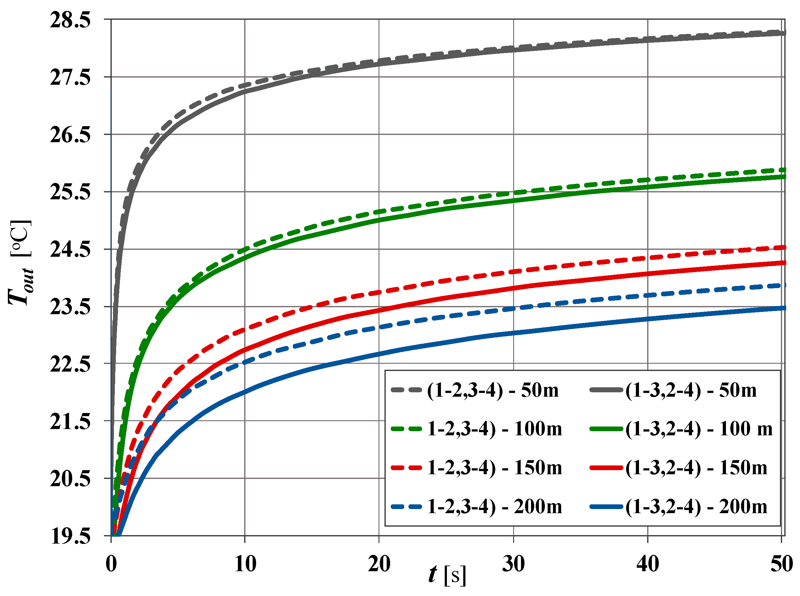
The plots in Figure 10 show time evolutions of the outlet fluid temperature, T_out, for different borehole lengths. To enhance the readability of the chart, the results are presented for time interval ranging between 0 and 50 h. The figure shows that plots of T_out are an ascending function of time and that the difference of T_out between the shallowest and deepest boreholes reaches 5 °C. It is evident that deeper boreholes give better thermal performance, i.e., lower outlet fluid temperature. Here, the configuration (1-3,2-4) again gives far better thermal performance than configuration (1-2,3-4), in particular for deeper boreholes.

The figure clearly demonstrates that the difference between T_out in two configurations significantly depends on the borehole length. While this difference at t = 50 h for a BHE with 50 m length is negligible (around 0.02 °C), it exceeds the 0.4 °C for a BHE with 200 m length. As shown in the previous section, this difference may increase for closer spaces between tubes. The figure indicates that for boreholes deeper than 100 m, the circuit arrangement can significantly affect the value of the BHE outlet temperature.

Table 7. Sensitivity of the thermal resistance and fluid temperature to borehole length variation.

		(1-2,3-4)				(1-3,2-4)
L	(Tin − Tout)	(Tf,ave − Tf,m)	Rb	ΔRb	(Tin − Tout)	(Tf,ave − Tf,m)	Rb	ΔRb
[m]	[°C]	[°C]	[W-1 m K]	[%]	[°C]	[°C]	[W−1 mK]	[%]
50	3.38	0.37	0.0669	−20.4	3.41	0.28	0.0654	−16.5
100	5.65	1.20	0.0841	0	5.75	0.91	0.0783	0
150	6.96	2.11	0.1103	31.2	7.19	1.64	0.0982	25.4
200	7.59	2.91	0.1432	70.4	8.01	2.29	0.1231	57.2

reports the sensitivity of (T_in − T_out), (T_f,ave − T_f,m), and the BHE thermal resistance to variation of the borehole length. The results support the statement that the difference between the influential parameters in two configurations increase remarkably with the borehole length. For instance, for a borehole with a length equal to 200 m, the borehole thermal resistance of the configuration (1-3,2-4) is 14.1% lower than that of configuration (1-2,3-4), which is almost double the existing difference for L = 100 m.

The comparison of obtained results indicates that the thermal resistance of configuration (1-2,3-4) is more sensitive than that of configuration (1-3,2-4) to the borehole length variation; for L = 200 m, the decrement percentage of the thermal resistance, ΔR_b, with respect to the case with 100 m length, increases to more than 70% in configuration (1-2,3-4), compared with 57% for configuration (1-3,2-4).

It is noteworthy that the difference between T_f,ave and T_f,m increases with the borehole length. As previously shown, this difference increases by decreasing the shank spacing. However, the increment caused by increasing the borehole length is by far larger than that caused by decreasing the shank spacing. Moreover, the discrepancy between values of (T_f,ave − T_f,m) in two configurations increases with the borehole length. For a BHE with L = 200 m, the difference between (T_f,ave − T_f,m) values of two configurations is 0.62 °C, while this value for a BHE with L = 50 m is only 0.09 °C.

Indeed, the deviation of T_f,ave from T_f,m caused by thermal short-circuiting leads to the greater deviation of the effective thermal resistance, R_b-eff, from the 3D thermal resistance, R_b-3D. To prove this, one can rewrite the Equation (10) as below.

$$R_{b-eff}=\frac{T_{f,ave}-T_{b,m}}{q_l}=\frac{T_{f,m}-T_{b,m}}{q_l}+\frac{T_{f,ave}-T_{f,m}}{q_l}=R_{b-3D}+\frac{T_{f,ave}-T_{f,m}}{q_l}$$

(11)

By substituting the energy balance of the fluid in the steady-flux condition in Equation (11), one gets:

$$R_{b-eff}=R_{b-3D}+\frac{L}{\dot{m}{c}_p}\frac{T_{f,ave}-T_{f,m}}{T_{in}-T_{out}}$$

(12)

This confirms that for a given BHE length and mass flow rate, the deviation of T_f,ave from T_f,m leads to the higher difference between the R_b-eff and R_b-3D.

Equation (12) allows a simple evaluation of the difference between R_b-eff and R_b-3D, taking into account the effect of the BHE length and the mass flow rate. It is evident from Equation (12) that for deeper BHEs or lower flow rates, the deviation of R_b-eff from R_b-3D could increase.

7. Thermal Effectiveness

In this section, the BHE thermal effectiveness rendered by each configuration is evaluated for different shank spacing and borehole length values. The energy exchange characteristic for the borehole could be quantified by employing the concept of the effectiveness coefficient of thermal energy. The BHE effectiveness coefficient, ε, can be defined as the ratio of the actual heat transfer to and from the BHE for a given inlet temperature to the maximum possible theoretical heat transfer between the circuit fluid and the surrounding ground [43]. This is given by:

$$\epsilon =\frac{{\dot{Q}}_{actual}}{{\dot{Q}}_{\max }}=\frac{\dot{m}{c}_p(T_{in}-T_{out})}{\dot{m}{c}_p(T_{in}-T_{g{d}_0})}$$

(13)

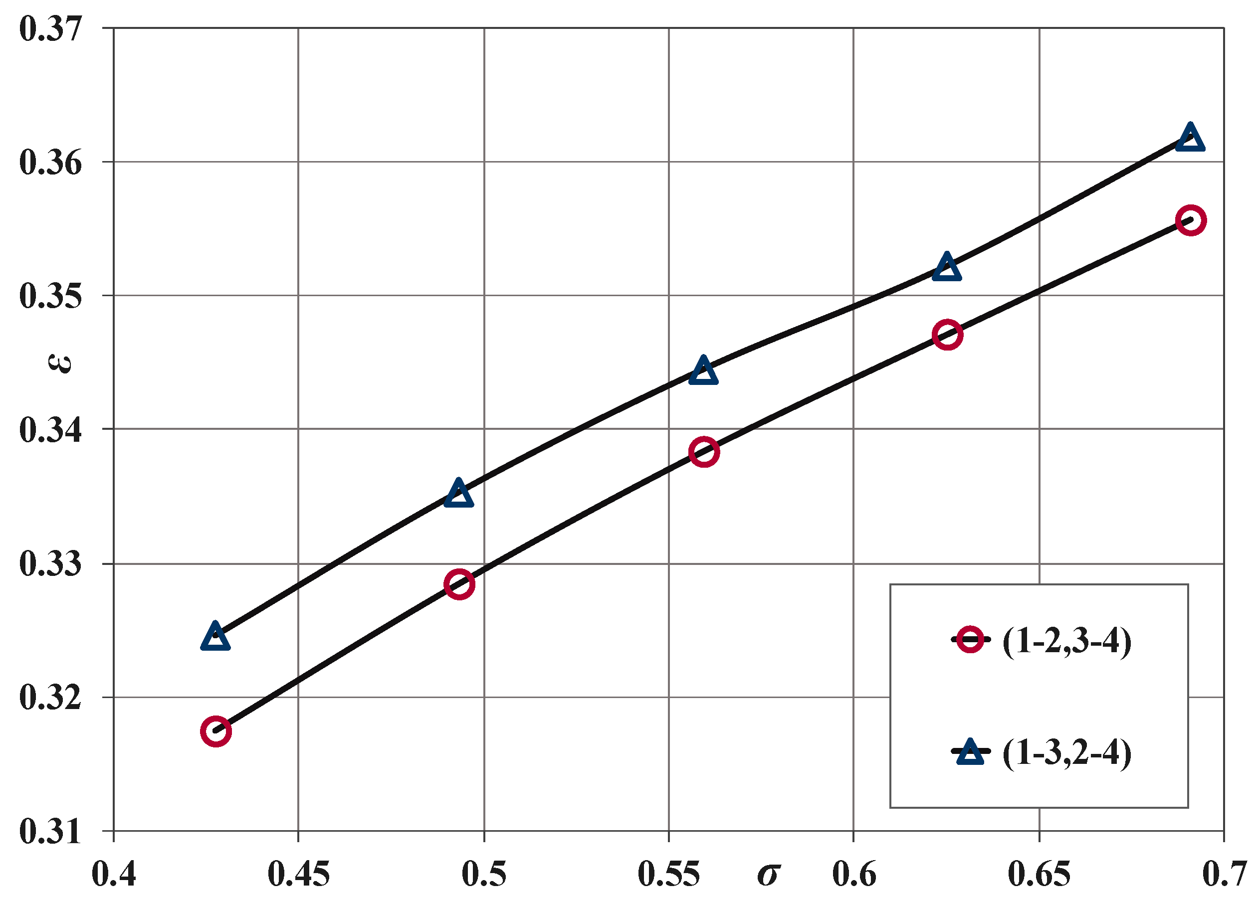
Figure 11 illustrates variations of ε with shank spacing in the steady-flux condition for both configurations of the BHE with L = 100 m. The figure shows that ε increases with dimensionless shank spacing, σ, and that configuration (1-3,2-4) gives a slightly higher ε compared with configuration (1-2,3-4). However, the increment of ε with shank spacing is insignificant; by maximally increasing the shank spacing (40 mm), the thermal effectiveness value increases almost 0.04.

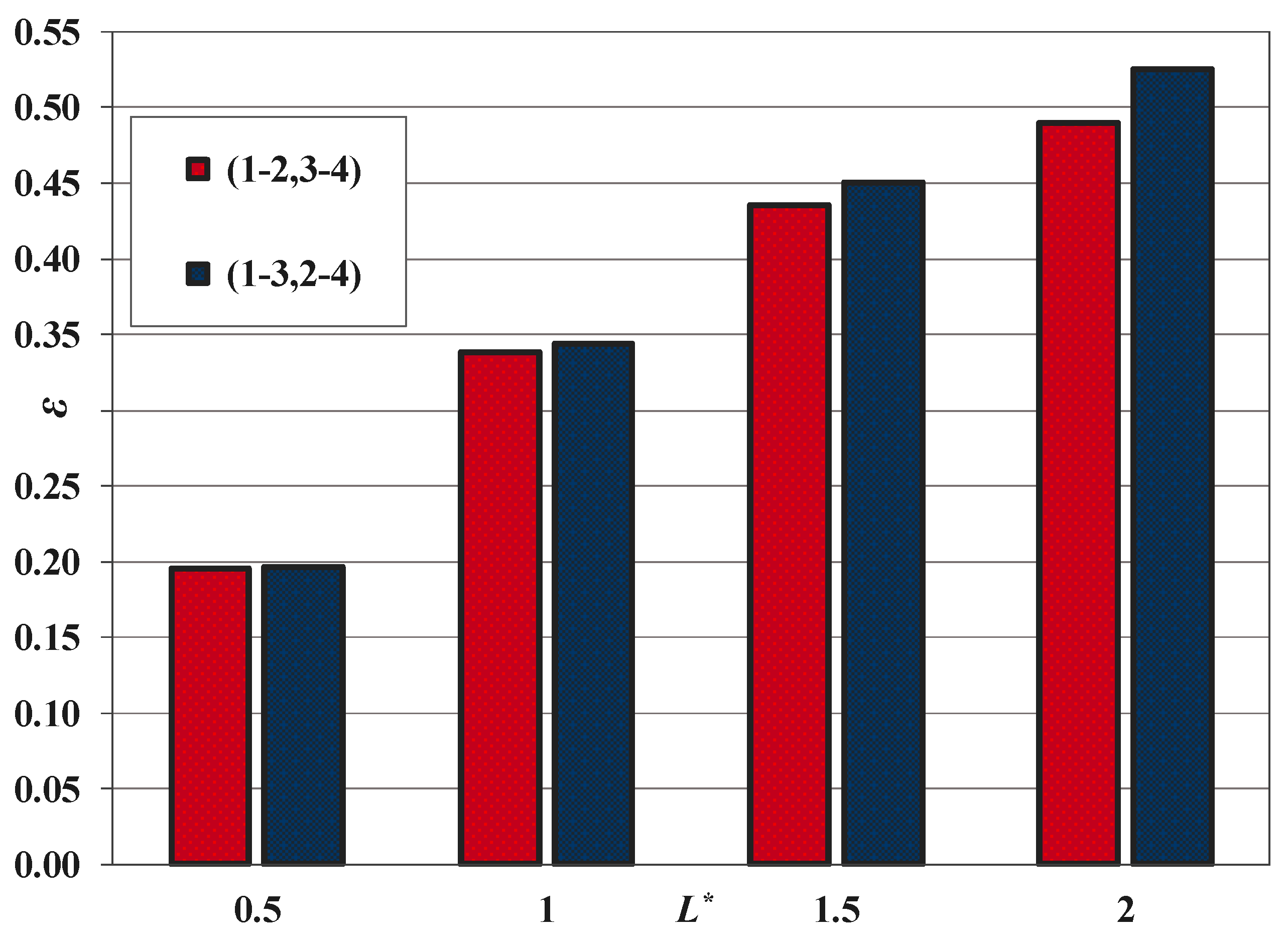
On the other hand, the column charts in Figure 12 show that the borehole length can dramatically affect the thermal effectiveness. The figure shows that the effectiveness coefficient increases by 169% by increasing the borehole length from 50 to 200 m. In addition, the chart indicates that the difference between the values of the ε in two configurations is small for shallow BHEs. However, this difference is remarkable for BHEs deeper than 100 m. It can, therefore, be concluded that the kind of circuit arrangement for deep BHEs is of significant importance.

8. Conclusions

The present study investigated relative changes in the thermal performance of double U-tube BHEs triggered by alterations in circuit arrangements, as well as the shank spacing and the borehole length by means of a series of 3D finite element simulations. The numerical model was validated against the analytical model based on the line-source method. In addition, the results obtained by numerical simulations were compared with those obtained through correlations deduced by linear regressions of a dimensionless coefficient. Three configurations for parallel arrangement of U-tubes were considered and differences in their thermal comportment were compared. The effective borehole thermal resistance and the temperature difference between the system inlet and outlet were treated as influential parameters to evaluate the thermal performance of the BHE.

The sensitivity of each configuration in terms of the thermal performance to shank spacing and borehole length variations was assessed. The impact of the thermal interference between flowing legs, namely thermal short-circuiting, on parameters affecting the thermal performance of the BHE was addressed. Deviations of the mean fluid temperature from the arithmetic mean of the inlet and outlet temperature were analyzed for various geometrical conditions. Furthermore, it was shown that this deviation is related to differences between the effective thermal resistance and the 3D thermal resistance. Finally, the energy exchange characteristic for the double U-tube BHE with different configurations was quantified by the employing effectiveness coefficient of thermal energy. The following remarks can be concluded:

• For a symmetric disposal of the tubes and equivalent mass flow rates, the thermal performance of configurations (1-3,2-4) and (1-2,4-3) could be considered as identical.
• Among all double U-tube configurations for parallel circuit arrangement, configuration (1-3,2-4) rendered the lowest BHE thermal resistance, the greatest difference in inlet and outlet fluid temperature, and consequently the best thermal performance. The discrepancy between values of the effective thermal resistance for two configurations reached over 14%.
• An analysis performed on configuration (1-2,3-4) by inserting an adiabatic surface between flowing legs showed that its lower thermal performance compared with other configurations is due to thermal short-circuiting, in particular for lower shank spacing values and higher borehole length values.
• Configuration (1-2,3-4) showed a slightly better improvement rate for thermal performance with increasing shank spacing and borehole length in comparison with configuration (1-3,2-4). In addition, regardless of the kind of circuit configuration, the borehole thermal resistance was quantitively more sensitive than the outlet temperature to variation of shank spacing.
• Due to the higher thermal interreference between tubes in configuration (1-2,3-4), the deviation of the averaged-over-the-depth mean fluid temperature from the simple average of the inlet and outlet temperature was considerable, in particular for lower shank spacing values and higher borehole length values. It was shown that this discrepancy could be related to the difference between values of the two different definitions of the BHE thermal resistance.
• The BHE length was more influential than shank spacing in increasing the existing discrepancy between the thermal performances of different configurations.
• The value of the borehole thermal effectiveness between two configurations may differ to a significant extent for BHEs deeper than 100 m, while this difference for shank spacing variation was scant.

The presented numerical model provides a practical tool to simulate and analyze the transient thermal comportment of U-tube BHEs for both short- and long-term operations. For future research, a possible direction is to extend this study in conjunction with variations of operational parameters.