Cost-Aware Design and Simulation of Electrical Energy Systems

Abstract

One fundamental dimension in the design of an electrical energy system (EES) is the economic analysis of the possible design alternatives, in order to ensure not just the maximization of the energy output but also the return on the investment and the possible profits. Since the energy output and the economic figures of merit are intertwined, for an accurate analysis it is necessary to analyze these two aspects of the problem concurrently, in order to define effective energy management policies. This paper achieves that objective by tracking and measuring the energy efficiency and the cost effectiveness in a single modular framework. The two aspects are modeled separately, through the definition of dedicated simulation layers governed by dedicated virtual buses that elaborate and manage the information and energy flows. Both layers are simulated concurrently within the same simulation infrastructure based on SystemC-AMS, so as to recreate at runtime the mutual influence of the two aspects, while allowing the use of different discrete time scales for the two layers. Thanks to the tight coupling provided by the single simulation engine, our method enables a quick estimation of various cost metrics (net costs, annualized costs, and profits) of any configuration of EES under design, via an informed exploration of the alternatives. To prove the effectiveness of this approach, we apply the proposed strategy to two EES case studies, we explored various management strategies and the presence of different types and numbers of power sources and energy storage devices in the EES. The analysis proved to allow the identification of the optimal profitable solutions, thereby improving the standard design and simulation flow of EES.

1. Introduction

In the design of large-scale electrical energy systems (EESs), cost is a dimension at least as important as the energy efficiency of the system: given the initial investment, in fact, users do want an effective solution that can provide a return on the investment in the shortest possible time.

Designing an EES encompasses a number of options, such as the choice of components (which power sources and which storage devices), their sizing, and particularly, their management (how the energy flow is controlled among all the actors), possibly in a way that is aware of the load profiles. The problem of optimizing the cost under an initial investment cost constraint is therefore a complex problem, as it involves both “physical” aspects (i.e., the dynamics of the various devices, their non-idealities, the electrical characteristics of the loads, etc.) as well as “cyber” issues (the algorithms that manage the flow of energy among these devices and the loads).

It is quite evident that accounting for (i) such a set of heterogeneous variables, (ii) numerous significant non-idealities, and (iii) complex inter-dependencies between components can only be handled effectively by the simulation of the EES as a cyber-physical system (CPS). This would allow one to describe accurate (power and cost) models for the components, fed by accurate traces of environmental data for the power sources, and exercised under realistic power demand traces [1,2]; on top of that, management policies modeled in software can evaluate a number of alternative scenarios. Although throwing all these aspects into an optimization problem would be possible [3], this could be done only using average quantities as representative values for the variables of the problem.

The literature presents many solutions for the simulation of these cyber-physical electrical energy systems (CPEES), with different levels of accuracy, complexity, generality, and flexibility [4,5,6,7,8]. Most of these approaches lack one fundamental feature which could be regarded as modularity. With this term we mean the possibility of separating the different layers of information to be tracked in the CPEES simulation. For instance, the analysis of the power flow (an “power layer”) could be carried out to extract information that could be used for different purposes by another “layer” of simulation that sits on top of that power layer. Such information could be used, for example, to track the reliability (e.g., the mean time to failure, MTTF, or the mean time between failures, MTBF) of the CPEES, using appropriate reliability models that depend on how energy is used and are fed by the power traces obtained by the simulation at the power layer. Alternatively, as done in this work, one could use the power traces to feed cost models to assess the overall economic balance of the system. In some cases, a user might want to have both layers (reliability and cost), while in others, one might be interested in only one of them. This degree of modularity requires a specific architecture of the overall simulation framework.

An interesting solution that follows this modular approach was proposed in [9], where the authors design a framework for the concurrent simulation of both functionality and extra-functional properties, yet in a different context. The work refers to smart electronic systems [10,11,12], which can be seen as small scale CPSs; here, the bottom layer of the simulation is the functionality; i.e., what the overall system does and its timing evolution in terms of digital signals. Layers built on top of this baseline layers (called “non-functional”) track other quantities (called properties), such as power consumption, temperature, and reliability, stacked in this order. The key for modularity in this work was the definition of a multilayer, bus-centric framework where each layer has a similar structure: each simulated quantity corresponds to a simulation layer, and the bus-centric organization in each layer implies the definition of a virtual bus, which conveys and elaborates quantity-specific information (i.e., power-bus, temperature bus, etc.) to ease synchronization and information exchange.

In this work we adopt the paradigm of [9] to use it to add support for a new “property”; i.e., cost. Cost is modeled as a new layer of the framework of the bus-centric approach: component-specific costs are estimated locally to each component, while the bus merges them and keeps track of the power balance and of any operation of the grid; i.e., to buy or sell power. We additionally extend the framework to focus on the simultaneous simulation of cost with the power layer, to reproduce the mutual interactions of the two properties, and to investigate such mutual inter-dependency.

Finally, we apply the extended framework to the design of a custom EES, that is used to highlight and investigate the characteristics of the proposed modeling and simulation approach.

The paper is organized as follows: Section 2 discusses the background, including related work and a brief introduction of the multi-layered framework of [9]. Section 3 illustrates how to build the cost-layer and the information exchanges with the other layers. The implementation of proposed simulation framework is introduced in Section 4. Section 5 exemplifies the overall approach on a reference EES case study to prove the effectiveness of the proposed solution, and Section 6 draws our conclusions.

2. Background

2.1. Cost Estimation for EES Systems

The estimation of the total cost (and the possible resulting economic benefit) of an EES should consider a number of cost items; namely, the initial investment, the runtime operation expenditures (i.e., maintenance and obsolescence), and the cost of energy consumption, which depends on the overall architecture and the load profiles. Once a comprehensive model is available, it will allow one to compare different solutions (mainly the allocation of the energy flow, and the choice and sizing of the components), so as to choose the most profitable one, by taking into account a number of constraints and of optimization goals.

Given its relevance in many domains (industry, residential, large-scale energy generation installations), the literature on the topic is quite rich. The most recent solutions proposed at state of the art are summarized in

Table A1. Overview of recent representative related works on cost estimation of EES Systems.

Ref.	Goal	Energy Models	Cost Models	Proposed Solution
[13]	Optimize energy storage configuration to minimize fuel costs	Simple linear models, e.g., PV power as function of area and rated power	Operation and maintenance, replacement, capital	Comparison of alternative configurations
[14]	Find sizing of EES components that minimizes levelized cost of electricity	Based on linear equations of rated power and capacity	Capital, operation and maintenance, replacement	HOMER [58] and artificial bee colony optimization
[15]	Optimal configuration while minimizing total net present cost	Simplified models of EES components (e.g., battery as a function of efficiency and depth of discharge)	Capital, replacement, operation and maintenance	Hybrid optimization genetic algorithm
[16]	Optimization of levelized energy cost and payback time, emission reduction	Simple linear models	Annual investment and replacement, emission reduction benefit	Particle swarm optimization to identify optimal component sizing
[17]	Minimize cost and improve reliability	Simple linear models, e.g., power sources as linear function of environmental quantity	Investment, replacement, operation and maintenance, electricity	Constrained optimization problem to determine capacity of power sources and storage
[18]	Optimization of annualized cost through dimensioning of EES components	Power sources as simple linear function of environmental quantities	Operation and maintenance, capital, replacement, electricity	Mixed integer linear programming applied to different scenarios
[19]	Optimal sizing of EES components to minimize levelized cost of energy	Accurate models, fixed power management policy	Capital, operation and maintenance, replacement	Genetic algorithm
[20]	Maximize electricity bill savings with optimal sizing of energy storage	Accurate model only of energy storage devices	Capital, electricity, replacement	Non-convex optimization problem plus exhaustive-search solution
[21]	Optimal sizing of EES components given pricing policies	Focus only on power source capacity and battery state of charge	Capital, operation and maintenance, electricity	Cataclysm genetic algorithm
[22]	Reduce cost of microgrid expansion considering impact of battery dynamics	Focuses on batteries, simple model of power sources	Capital, electricity, annualized cost	Mixed integer linear programming
[23]	Optimize battery sizing given battery bank degradation cost	Models only battery aging, fixed power management policy	Electricity, battery degradation	Linear optimization method
[24]	Optimize battery size and scheduling taking into account costs and loads	Simple linear models, input traces for power sources	Electricity, battery capital cost	Convex programming method
[25]	Find sizing of EES components plus operating strategy to minimize costs	Simple models, based on rated power, efficiency coefficients, area occupied by PV modules, etc.	Annualized system cost	Mixed integer linear programming model solved with CPLEX
[26]	Optimization of battery management to minimize electricity cost and carbon dioxide emissions	Focuses on battery state of charge, no model of other EES components	Electricity, emissions equivalent cost	Multi-objective optimization (energy cost and emissions)
[27]	Co-scheduling problem of HVAC control and battery management	Detailed model only of batteries (power sources as input traces, converters as efficiency coefficients)	Electricity, battery degradation	Minimize total cost with the convex optimization tool CVX
[28]	Utility scheduling to minimize total operational cost	Storage devices modeld only as their lifetime, power sources as input traces	Electricity, degradation, pricing schemes	Nonlinear mixed integer optimization to determine schedule of batteries and supercapacitors
[29]	Determine optimal power management policy to reduce operation and emission costs	EES components as min-max constraints for the optimization	Operation and maintenance, electricity	Particle swarm optimization
[30]	Balance total power generation w.r.t. load and minimize total operation cost	Capacity and scheduling as goal of optimization	Capital, operation and maintenance, electricity	Integer linear programming with CPLEX
[31]	Construction of optimal scheduling to optimize usage of storage and grid	EES capacity as constraints and object of optimization	Levelized cost of energy	Predictive optimization given a graph of alternatives
[32]	Techno-economic model to determine optimal capacity of PV system and battery storage	Simple models, e.g., PV as linear function of irradiance and temperature	Capital, operation, payback time	Particle swarm optimization
[33]	Optimal sizing of EES components to maximize profit	Accurate model only of PV modules	Capital, operation and maintenance, electricity	Dynamic simulation to evaluate impact of electricity tariffs
[34]	Feasibility study of wind/PV hybrid system	Accurate model only for PV modules	Capital, operation and maintenance, replacement	Simulation based on MATLAB and HOMER [58]
[35]	Operation cost minimization with different pricing mechanisms	Simple linear models	Annualized cost of system components	Based on HOMER [58]
This	Estimate mutual impact of power dynamics and costs to reach effective design of EES (Section 3.3 and Section 5)	Level of detail can be tuned by user, allows one to have high level of accuracy of component dynamics (Section 2.2 and Section 4)	Capital, profit, depreciation, operation and maintenance, electricity, net and annualized cost (Section 3)	Simulation-based, allows efficient construction and evaluation of alternative configurations (Section 5)

(moved to the Appendix A not to interrupt the natural flow of the paper). The Table highlights the goal of each work, how EES components are modeled, the considered costs, and most importantly, the solution proposed by each work, which mostly fall under two categories: optimization-based approaches and simulation-based approaches.

Optimization-based solutions use analytical or empirical equation-based models of the power characteristics of EES components and the corresponding costs, and formulate the problem into the constrained optimization of a given target; e.g., maximization of power production, or minimization of a cost function [13,14,15,16,17,18,19,20,21,22,23,24,25,26,27,28,29,30,31]. Unfortunately such approaches suffer from many limitations. Given that the focus is optimization of some economic parameter, the evolution of EES components is considered only as a byproduct: either as a constraint or an optimization goal [29,30,31], or as a dimension of the problem that can be reproduced with simplified models or even simple input traces [13,14,15,16,17,18,24,25,28,32], thereby sacrificing accuracy to simplify computation. When accurate models are adopted, they are restricted to a subset of the components considered of interest (e.g., only batteries or PV modules), while the other EES components are either ignored or modeled with simplistic equations [20,21,22,23,26,27]. Few works take into account the power management strategy used to activate power sources and energy storage devices. When this happens, the goal is determining the optimal day-ahead scheduling of energy storage devices, thereby preventing the comparison of different power management strategies [26,27,28,29,30,31]. As a result, power dynamics are always considered as a minor dimension of the problem (i.e., a constraint, an optimization goal, or an input), and the mutual impact of power and cost is completely lost. Finally, these approaches provide one solution (or a few) and do not easily allow a comparative analysis of various solutions, nor the sensitivity of a solution with respect to some of the parameters.

Simulation-based approaches optimize EES design from an economic perspective based on dynamic simulations of alternative configurations [33,34,35]. The goal is the evaluation of the impact of electricity pricing, the feasibility of the constructed EES, or the evaluation of the most economical alternative. However, once again the focus is on the economic dimension, thereby adopting gross grain temporal scales (e.g., 1 h time steps) and restricting accurate modeling only to specific classes of EES components of interest (e.g., PV modules [33,34]). Finally, the focus is restricted to only one direction of the mutual impact between the cost dimension and power dynamics of the EES under analysis, which are evaluated strictly sequentially, depending on the causality of interest.

The main limitations of the aforementioned approaches are thus the adoption of abstract and simplistic models of EES components and the gross grain temporal scale: the energy dimension is thus modeled with a very low level of detail, thereby missing important intrinsic dynamics of the EES components, together with the modeling of inefficiencies and of realistic operating conditions. Additionally, cost and power evolution are never considered as mutually interacting dimensions, thereby missing important dimensions of the analysis.

The work proposed in this paper can be viewed as a different perspective; while it is a simulation-based approach, it leverages results of an independent simulation of power traces, which can use models with variable accuracy and possibly with different time scales; these power traces are then fed into the various models of different cost items (where they are power-dependent), which can vice versa influence and impact the power dimension. This kind of modular approach is not, however, the result of two distinct simulation environments, but both power and cost information can be derived by concurrently simulating them: this allows one to expose all mutual dependencies between power and cost, and thus to improve the design of EES with a more informed view of all the variables. There is one study [36] that focused on the modeling the different components in the EES by using a different model of computation (MoC) in one simulation framework by using SystemC-AMS. Cost is indeed mentioned in that study, but there is no indication of how the cost models of that work are linked to the power simulation. These are simply obtained by a post-processing of the power traces, as done in most related works. Our proposed simulation framework speeds up the design-time optimization process and has different methods to evaluate the power flow and economic benefit of EES by concurrently simulating the two quantities. The key for such a modular and concurrent simulation approach is described in the following section.

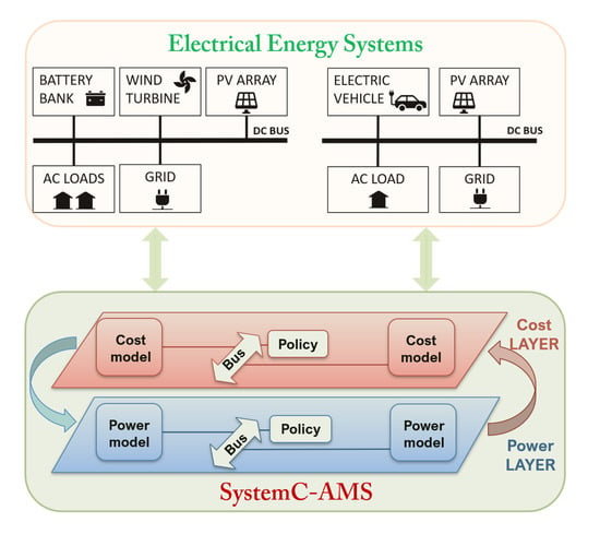
2.2. A Multi-Layered Approach for Functional and Extra-Functional Simulation

The simultaneous simulation of the various aspects of a system requires the construction of frameworks that integrate different views of a system in a single run. The work in [9], which targeted smart electronic systems, proposed an effective methodology that allows the simulation of system functionality together with its power, thermal, and reliability evolution.

The approach proposed in [9] envisions a multi-layer, bus-centric framework (depicted on the left-hand side of Figure 1, adapted from the original paper): multi-layer because it has a stacked layers structure; each layer is associated with one simulated characteristic of the system (called property). Bus-centric means each property is simulated with a virtual bus in each layer, used to update the property-specific status of the system. All simulated properties are thus reduced to this common structure, thereby easing synchronization and information exchange. The goal is indeed to avoid the construction of co-simulation frameworks, and to rather simulate all layers in a single run by falling on the same implementation language; namely, SystemC-AMS.

Each layer is fixed to a single generic underlying architecture, of which the layer-specific bus is the central element, used to carry information between components (layer-specific signals). Such information is specific of the property under analysis in the layer (e.g., voltage and current for the power layer). Each component in the system corresponds to a model in each layer, to capture the property-specific evolution over time of the component. The layer-specific bus aggregates the property-specific information of each component to control the information flow and update the overall property-specific information. Layers can additionally share information (inter-layer signals) to mutually influence each other. Notice that signals can go in both directions; i.e., they can be forwarded to upper layers, as signals that are needed to carry out the simulation at that layer (solid lines); but signals can also be fed back to lower layers as information that can make the lower-level simulation more accurate (dotted lines). In the context of [9], for example, the former type of signals could be power consumption signals forwarded upwards to compute the temperature map of the system; the latter type could be the same temperature maps, which could impact the power consumption of some of the components. Most importantly, when the layers run at different time scales, time converters can be introduced to convert the signals towards coarser or finer time scales. For instance, while it makes sense to measure the functionality of an electronic system at the nanosecond scale, this is not a required granularity for power simulation, and can be even more relaxed for the analysis of the thermal flow.

Not shown in the figure, there are also layer-specific description data that are strictly referring to that layer and are needed as a sort of “context” of the simulation. In the temperature layer of [9], these data could refer either to the physical locations of the components, which affect the thermal flow, or to the characteristics of the materials (type, thickness, etc.) constituting the system itself.

This paradigm proved to work very well for the simulation of the different views of a smart system, thanks to its scalability and to the simultaneous evolution of the different system properties, which thus can react simultaneously the one to changes of the other.

For this reason, in this work we tried to fit the above-described paradigm to the co-simulation of power and cost of an EES, with the objective of exploiting its two main benefits; namely, modularity and generality. Notice that the contribution of this work is showing that the layered, modular framework of [9] is not a customized architecture, but its paradigm can be extended to other quantities: in this specific case the operational costs of an EES. The work of [9] was applied to small-scale electronic systems, where the non-functional properties were (from bottom to top; see Figure 1 in the manuscript) power, temperature, and reliability. Our work aims at demonstrating the general applicability of the modeling and simulation paradigm of [9] to the context of large-scale EES, and can add different non-functional properties that the properties in this work are power and cost. The right-hand side of Figure 1 shows how the generic bus-based layered architecture maps to our specific context. Since we focus on EES, the first layer of the simulation stack coincides with the power layer. In some sense, this represents the equivalent of “functionality” in the original version; that is, the lowest abstraction level of the semantics. On top of the power layer sits the cost layer, which receives power flow information (used to update the power-dependent cost items, such as electricity cost) and returns cost information to the power layer, which can be used to implement policies in the power bus to decide the optimal power flow among the various components.

Time converters are also expected, since some updates of some of the cost items might generally have different time granularity with respect to power updates, which in the finest granularity are updated every 15 min (as in the most accurate meters).

In the conceptual architecture of Figure 1, the power layer is fundamentally working just as described in [9]; even if components are different in their power scale (100 s of Watts vs. milliwatts), their interfaces and interaction are the same. The cost layer, conversely, is an original layer and its implementation within the constraints of the layered structure demonstrates the claim of modularity of the architecture. In the next section, we will describe the cost models and the technical details to incorporate the cost layer within the template of Figure 1.

3. Modeling of Cost

Calculating the life-cycle cost of the EES is an accurate and sound way to estimate the overall cost spent on an asset over the course of its useful life, thereby including the initial capital costs, the projected operating costs, and the maintenance costs, plus possible disposal costs or final residual values of the asset. This Section maps the characteristics of the various models of the life-cycle cost with respect to the layered structure outlined in Section 2.2.

3.1. Main Characteristics of the Cost Layer

The cost of the whole EES is a combination of component-specific cost items—that is, that can entirely be determined locally for each component (e.g., initial investment cost, operation, and maintenance cost); and of global costs—that is, costs that require an aggregation to be computed; this is essentially the case for electricity cost, whose computation implies the calculation of the balance of the power flow. Therefore, the adoption of a bus-based architecture for the cost layer is relatively natural and straightforward:

• Each component computes its “local” costs over time;
• All individual costs are conveyed to the cost bus;
• The cost bus estimates additional global costs, i.e., due to energy balance with respect to the grid;
• The cost bus determines and keeps track of the total balance over time.

The characteristic information managed in this layer is cost, interpreted as a numeric value in some currency. Cost is thus the only layer-specific signal that connects all components to the layer-specific bus, and all components are directly connected to the cost bus. Notice that this architecture may not reflect the actual physical organization among the components in the actual EES. For instance, in the real-world EES, a certain component may be connected to the physical power bus through a DC-DC converter; nonetheless, in this virtual cost layer, both the component and the DC-DC converter are independently connected to the cost bus. Figure 2a shows a pictorial representation of the general structure of the cost layer.

3.2. Cost Models

This Section details the various cost components by category, and it maps them to the cost layer template. Notice that the presence of multiple cost models makes the cost signal connecting components to the bus rather an array of cost values, as sketched to Figure 2a, where each array element denotes one cost category listed hereafter. In the following, we will use uppercase letters C to denote cumulative costs; i.e., costs whose definitions encompasses the time intervals over which they are accrued. Lowercase c denotes instantaneous costs. The former are expressed in currency × time, e.g., $ × year, and the latter in currency.

3.2.1. Component-Specific Costs

We consider three main component-specific cost items. Since our focus is on small to medium-scale EESs (such as those in residential installations), we ignore here disposal costs or final residual values as they can be regarded as marginal. These could be, however, easily incorporated without any conceptual difficulty.

Initial Capital Cost

Initial capital cost is the initial investment for the purchase of a component at time zero. This expense is computed for component i by considering its unit cost $C_{unit,i}$ and its cardinality $N_i$:

$$C_{capital,i}=N_i·C_{unit,i}$$

(1)

where $C_i$ is the cost of one unit of component i; $N_i$ is the number of units of i. We decouple the two terms to allow the possibility of tuning the size of components in the exploration. Many components can in fact being seen as modular (e.g., a PV panel consists of a number of PV modules, a battery pack of a number of cells, etc.).

Time-Dependent Capital Cost

Time-dependent capital cost describes the decrease in the value of a component over its useful life as a consequence of obsolescence and/or wearing, and it is in general proportional to its initial capital cost. We consider two types of components, depending on how their loss of value is defined. A first category corresponds to components that have a maximum expected duration; examples are, for instance, PV panels and wind turbines, whose datasheets typically define maximum operational life. For this class, we call this cost depreciation cost, defined for component i as:

$$C_{depreciation,i}\left(t\right)=C_{capital,i}·CRF·\frac{t}{T_s}$$

(2)

where $C_{capital,i}$ is defined as in Equation (1), and $T_s$ serves as a time normalization factor and it denotes the number of simulation samples ($\Delta T$) per year, in order to express the depreciation over each sample time (e.g., if the $\Delta T$ is 1s, $T_s=3600\times 24\times 365$). $CRF$ is the capital recovery factor, a ratio used for estimating the present value during the lifespan of a system if invested at a particular interest rate [37]. $CRF$ is expressed by:

$$CRF=\frac{R·{(1+R)}^n}{{(1+R)}^n-1}$$

(3)

where R is the interest rate, and n denotes the number of years of operations of the system (i.e., component lifetime).

A second class of components has instead a lifetime not defined a priori, but  rather determined by their usage characteristics; this is for instance the case of batteries, whose lifetime is defined upon reaching a given value of usable capacity, which depends on several usage-related factors [38]. To distinguish from the former category, we call the time-dependent capital cost for this class as wear-out cost, defined for component i as:

$$C_{wout,i}\left(t\right)=C_{capital,i}·\frac{L\left(t\right)}{L_{max}}$$

(4)

where $L\left(t\right)$ is the loss of “functionality” over time and $L_{max}$ is the maximum value of the loss after which the component is considered not functional and it needs to be replaced. Thus, when $L\left(t\right)$ reaches $L_{max}$, the entire capital cost has been consumed.

$L\left(t\right)$ clearly depends on the type of component and requires an ad-hoc model. Using a battery as an example, $L\left(t\right)$ will be the capacity loss due to both calendar and cycle aging, which are affected by several parameters [39], most of which can be attributed to how the power is drawn from the battery, and thus from information derived from the power layer. $L_{max}$ is the maximum capacity loss before the battery is considered as depleted (usually a loss of 20% from the initial capacity). This information must be provided at runtime by power simulation, as will be explained later in this Section.

In summary, the time-dependent capital cost depends on the type of component; the term $C_{capital,i}\left(t\right)$ will correspond to either Equation (2) or Equation (4) depending on the characteristic of component i.

Operation and Maintenance Cost

Another time-dependent cost is the one due to operation and maintenance [40] that includes both scheduled and major corrective maintenance. This cost is component-specific, as it strictly depends on the characteristics of the component (e.g., it may include periodical cleaning, wiring replacement, and screw and bolt tightening). To this extent, many definitions of this cost are available.

$$C_{operation,i}\left(t\right)=C_{operation,yearly,i}·P_i\left(t\right)·\frac{t}{T_s}$$

(5)

where $C_{operation,yearly,i}$ is expressed in $/kW/Year; $P_i\left(t\right)$ is the instantaneous power flow related to different components i; e.g., the power generation of PV modules and power provided by the battery pack. $T_s$ is the time normalization factor defined as in Equation (2). The $C_{operation,i}$ includes the base cost of element replacement inside each component during its operating lifetime.

3.2.2. Bus Models

The functions of the cost bus are two-fold; firstly, it calculates the costs that depend on the overall power flow of the EES; i.e., the cost of electricity that is bought (and sold) over time from the grid. Secondly, it computes some global cumulative metrics to be used for the exploration of design alternatives or for computing the sensitivity with respect to some parameters of the EES.

Electricity Cost

Electricity cost is the instantaneous cost related to the money paid to (or received from) the utility provider as an effect of the total power balance in the system. This cost can be modeled as:

$$c_{elec}\left(t\right)=p_E\left(t\right)·\frac{E\left(t\right)}{{\eta }_{conv}}$$

(6)

where $E\left(t\right)=P\left(t\right)·\Delta t$ is the energy to be bought (or sold) at time t; $P\left(t\right)$ is the instantaneous power demand (positive or negative), which refers to the total balance of the EES, and its sign determines whether the power is being bought ($P\left(t\right)>0$) or sold ($P\left(t\right)<0$). $p_E\left(t\right)$ is the instantaneous electricity price (in currency/kWh); its value depends on the sign of $P\left(t\right)$:

$$p_E\left(t\right)=\left\{\begin{array}{cc}{p}_{E,buy}\hfill & \mathrm{if}P\left(t\right)>0\hfill \\ p_{E,sell}\hfill & \mathrm{if}P\left(t\right)<0\hfill \end{array}\right.$$

where typically $p_{E,sell}<p_{E,buy}$. ${\eta }_{conv}\le 1$ is the efficiency of the conversion process; i.e., how the nominally consumed energy $E\left(t\right)$ is actually perceived [2].

Given that Equation (6) depends on the overall power flow (production vs. demand) of the EES evolution, this cost can only be computed by the cost bus, that, by collecting the individual signals from the components can have a global perspective on the system.

Net Cost

The first global metric computed by the cost bus is net cost over time; i.e., simply the sum of all cost components:

$$C_{net}\left(t\right)=\sum _{\tau =0}^t\left(c_{elec}\left(\tau \right)\right)+\sum _i\left(C_{capital,i}\left(t\right)+C_{operation,i}\left(t\right)\right)$$

(7)

including, thus, time-dependent capital costs, operation and maintenance costs, and the cost of electricity until time t. Notice that the total electricity cost is obtained by integrating (summing) the $c_{elec}$ component over the time interval $[0,t]$, whereas the other components already include the time interval in their definition.

Annualized Cost

The annualized cost of an EES is the cost that, if it were to occur equally in every year in the system lifetime, would give the same net present cost as the actual cash flow sequence associated with the system:

$$C_{annualized}=\frac{C_{net}\left(t_{MAX}\right)}{{\displaystyle \sum _{t=0}^{t_{MAX}}}{P}_{PS}\left(t\right)}$$

(8)

where $t_{MAX}$ is the maximum system lifetime, and $P_{PS}\left(t\right)$ is the power produced by the EES power sources over the same interval. The equation considers all costs from the beginning of simulation to the end of system lifetime, and divides them by the total produced power, with no distinction between whether such power has been used to satisfy load demand or to sell power to the grid.

This cost basically returns the average cost per kWh of consumed energy produced by the system: it is thus a useful metric to compare alternative configurations of the EES and to have a picture of which configuration is more convenient than the others.

Profit

The net cost provides an indication of the total cost over a given time interval. When exploring different design alternatives (EES architectures, policies), a most useful metric is the actual profit of a given configuration. Defining a profit would, however, require to set a baseline to compare against; since the key element that has the most sizable impact on profit is the presence of renewable power sources, our definition of profit focuses on the net balance of the energy provided from power sources to the load and not requested from the grid (at the price $p_{E,buy}$). From this energy we need to subtract the net cost defined in Equation (7) .

$$Profit\left(t\right)=\sum _{\tau =0}^t\left(p_{E,buy}\left(t\right)·\frac{E_{ps2load}\left(t\right)}{{\eta }_{conv}}\right)-C_{net}\left(t\right)$$

(9)

Clearly, the profit is monotonically increasing with t during the lifetime of EES. The positive value of profit illustrates the given configuration can bring real benefit to the users, while the negative value indicates the given configuration is not a profitable one.

3.3. Interaction with the Power Layer

As stated in the previous section, some cost models depend on the power flows in the EES. The concurrent simulation of the cost and power layer is, therefore, essential to get an accurate estimation of the total EES costs. The generic inter-layer interaction depicted in Figure 1 shows generic connection between two layers. However, there are distinct types of interactions among the power and cost layers.

The first one involves an individual component in the two layers (Figure 2). The power model of a component $C_i$ sends the following information to its cost model:

• The time-dependent capital cost requires information about the current loss of functionality of the component L, and the maximum accepted loss $L_{max}$ (Equation (4)). Both values are known at the power layer: $L_{max}$ is a configuration value used by policies to determine when the component reached the end of its lifetime; L is a value that is constantly updated at simulation time to correctly estimate the behavior of the component. Using again the example of a battery, this would be approximated by the full cycle equivalent [41], i.e., the number of equivalent full charge-discharge cycles, which can be computed by just knowing the nominal battery capacity and the instantaneous power drawn.
• The operation and maintenance cost strictly depends on the power produced or stored by a component over a given time interval (Equation (5)); the power layer naturally keeps track of this quantity during simulation.

The second type of interaction involves the two buses as it concerns aggregate information (Figure 2c). The power bus forwards to the cost bus the following information:

• The energy balance over time $E_{TOT}$, taking into account the difference between the power provided by power sources and the power demand to guarantee the load operations. This quantity allows one to compute the electricity cost over time (Equation (6));
• The total power produced over time by power sources $P_{PS}$, useful for the estimation of the annualized cost (Equation (8)).

There is, however, also a feedback flow from the cost bus to the power bus. The former can in fact provide information to the power layer that can be used to design and apply specific power management policies. Examples of such information are:

• The current price of electricity: at times, the price of electricity may be so low that it makes convenient to recharge all energy storage elements (e.g., battery packs), and use the stored energy to power the system when electricity price is higher.
• Data on wear-out and/or depreciation in the form of alarms or warnings that can be used to force the replacement of some components.

The next section will present the implementation details (software infrastructure, timing model, etc.) of the overall intra-layer and inter-layer signal interaction.

4. SystemC-AMS Implementation

In order to replicate the approach proposed in [9], the proposed framework has been implemented in SystemC-AMS. Section 4.1 provides a brief introduction to SystemC-AMS, while Section 4.2 explains the reasons behind this choice and explains how SystemC-AMS has been adopted in this context.

4.1. SystemC-AMS

SystemC-AMS is the extension of SystemC for modeling analog and mixed-signal systems [42]. SystemC-AMS provides three different models of computation (MoC) to cover various domains as indicated in Figure 3.

Timed data-flow (TDF) models are scheduled statically by considering their producer-consumer dependencies in the discrete time domain. Each TDF module is characterized by a simulation time step, which is used by the TDF solver to insert timed activation events in the standard SystemC event queue. This ensures efficient computation, as it avoids any runtime dynamic event management. Continuous time models can be modeled with two abstraction levels. Linear signal flow (LSF) supports the modeling of continuous time through a library of pre-defined non-conservative primitive modules [43] (e.g.  in Figure 3 derivative and integrative, respectively). The electrical linear network (ELN) MoC models the electrical network by connecting the instantiation of predefined primitives (e.g., in Figure 3, capacitor and voltage source, respectively). All such abstraction levels are handled by the same simulation kernel that derives the system of equations to be solved over time and estimates system evolution.

4.2. SystemC-AMS Implementation of the Proposed Solution

SystemC-AMS is selected as the reference language for heterogeneous modeling for several reasons. The provided multiple abstraction levels unify the modeling work in a wide range of domains by using a single language: models can be built by choosing the most suitable abstraction level, and native converters can be exploited to simulate different abstraction levels simultaneously. SystemC-AMS also has the characteristics of a modular one, in that it divides the definition of interface and implementation, and is a IEEE standard language; thus, it can be easily extended and free from compatibility and reuse issues.

The flexibility of SystemC-AMS allows one to easily integrate the power models and the cost models. Figure 4 shows an example of a component implementation of a battery that is used in the remainder of this section as a reference. Each EES component is instantiated as a SystemC-AMS module (SC_MODULE, Figure 4, left) that internally instantiates one SystemC-AMS module for the power model and one for the cost model (line 5). This solution avoids forcing the fact that both models follow the same abstraction level and leaves maximum flexibility in the choice of the implementation style. The interface of the top level module includes the layer-specific signals of power (line 2) and cost (line 3) that will be bound to the corresponding ports of the layer-specific buses.

The interface of the power and cost modules includes the layer-specific signals (e.g., in case of the cost layer, one port per cost computed by the component, line 45) and the inter-layer signals, used to communicate with the other layer (line 22 for the signals propagated from the power module to the cost module). This naturally enables inter-layer communication: thanks to the encapsulation of both power and cost models in a single top level SystemC module, inter-layer communication signals are set as TDF signals, binding the property-specific ports of the modules (lines 4 and 14–16).

The implementation of power models in SystemC-AMS has been discussed in many works at the state of the art that proved that SystemC-AMS can find a good trade off between accuracy and simulation time [36,44,45]. The presence of multiple abstraction levels allows one indeed to adopt for each power model the most suitable solution; e.g., ELN for circuit or circuit-equivalent models, TDF for equations, and LSF for dynamic models. In the case of Figure 4, the power model adopted for the battery is the circuit model proposed in [38] that is implemented as a network of connected ELN primitives (e.g., $Ib$ is a current source, lines 23 and 30–32; $Cnom$ is a capacitor, lines 25 and 34–35).

Modeling the cost equations detailed in Section 3 is straightforward, as they can be easily mapped on C++ functions and primitives, encapsulated by the TDF semantics of SystemC-AMS. The right-hand side of Figure 4 shows a snapshot of code: the processing function of TDF repeatedly evaluates the cost models of the battery over time, in terms of capital cost (line 50), real-time capital cost (line 51), and operation and maintenance cost (line 52).

Note that the separation of the power model and the cost model in two different SystemC-AMS modules allows one to decouple their activation frequency. Power models require a fine grain activation time step (in the order of 1s down to 1ms) to accurately evaluate the internal dynamics of the component. Vice versa, the cost models allow a larger time step, so as to reduce the computation overhead. As a result, the activation time step of the two modules is different (lines 41 and 56, respectively), and the inter-layer signals are handled with a conversion between different time scales.

5. Simulation Results

All simulations reported in this section have been implemented in SystemC-AMS 2.1 and run on a server installed with Intel Xeon 2.40 GHz CPU (16 cores, 2 threads each) and 128GB RAM, with Ubuntu operating system 18.04.1.

5.1. EES Case Study 1

As an example case study, we used a grid-connected EES built upon the prototype of [46], and sketched on the left hand side of Figure 5. The EES includes a wind turbine, a photovoltaic (PV) array, a battery pack, various AC loads, a common DC bus, and the necessary converters.

Table 1. Characteristics of prototype EES components.

Component	Unit Rated Electric Characteristic	Cardinality (#)	Overall Rated Electric Characteristic
Wind Turbine	10 kVA	1	10 kVA
PV Module	57 V 5.49 A	30	10 kW
Battery Cell	3400 mA 3.7 V	40 × 60	200 Ah 144 V

and

Table 2. Initial capital cost and nominal lifetime of EES components.

Component	Unit Capital Cost ($)	O&M Cost ($/kW/Year)	Nominal Lifetime
Wind Turbine	19,500.00	15	20 Years
PV Module	675.00	15	20 Years
Battery Cell	2.50	10	SOH $\to 80\%$

report the main characteristics of the EES components, in terms of rated power and costs, respectively. The right hand side of Figure 5 shows the mapping of the case study to the proposed two-layer approach. The following subsections will detail the construction of the power and cost layers.

5.1.1. Power Layer

In the power layer, each EES component is described by a model. More specifically:

• The wind turbine is modeled with a mechanical model, proposed in [47];
• The PV array is modeled with a model of a single PV module, built by adopting the solution in [48], scaled up to the size of the PV array;
• The battery pack is based on the circuit-equivalent model in [38] (which models a single battery cell), scaled up to the size of the pack;
• AC loads reproduce power consumption of a residential community including 15 houses [49];
• Converters are modeled in terms of their conversion efficiency as introduced in [50];
• The grid component is used only to keep track of the power balance between demand and supply, and of any inefficiency introduced by the presence of a transformer between the grid and the power bus.

Table 1 collects the most relevant power characteristics of these components, plus the initial cardinality (# of elements) considered in the initial installation.

The power sources need input traces of irradiance and wind speed, which have been downloaded from the datasets of the National Renewable Energy Laboratory’s (NREL’s) Measurement and Instrumentation Data Center (MIDC) [51]. The time scale of irradiance and wind speed traces (one sample per minute) is longer that those of the load (one sample per second). We adopted the conversion methodology proposed in [9] to solve the issue of different time resolutions.

The power bus implements an initial non-cost-aware energy management policy similar to the one proposed in [52]: AC loads are satisfied by the renewable power sources whenever possible, and the battery pack is used to compensate whenever necessary (until its state of charge reaches a minimum of 10%). If the sum of energy stored in the battery pack and the power generated from the power sources cannot satisfy the AC loads, the houses purchase the missing energy from the grid. Otherwise, if the demand of the AC loads is less than the total power generation of the power sources, the unused power is used to charge the battery pack until it reaches 90% SOC, and then it is sold back to the grid.

5.1.2. Cost Layer

In the cost layer, only some components of the EES are relevant from the cost perspective. AC loads are not considered as a “variable,” as they are assumed to be given upfront in terms number and type; as such, they are not associated with a cost model, as they do not contribute to the overall economic evolution. Therefore, loads are an input of the system; i.e., a trace of the input power demand over time.

Another difference with respect to the power layer is that all costs connect to the grid; i.e., the costs of buying/selling energy to the grid, are taken into account inside the cost bus; it is not, therefore, necessary to include a specific component for the grid.

Thus, the cost layer features three components: the two power sources (i.e., the wind turbine and the PV array) and the energy storage (battery pack). Table 2 reports all cost information for such components. All components model their initial and time-dependent capital costs (Equations (1) and (2) or (4)) and their operation and maintenance cost (Equation (5)). Note that the operation and maintenance cost is expressed in terms of $/kW/Year, as it considers the annual routine operating and maintenance costs, and not accidental inside parts replacement. The interest rate used in Equation (3) is 7% for all components, and the CRF is thus set as 0.094.

The main difference between the models of the components is in terms of their time-dependent capital cost:

• The wind turbine and the PV array are considered as fixed lifetime components (with lifetime 20 years, as derived from their datasheets); thus, their time-dependent capital is modeled as in Equation (2).
• The battery pack has a variable lifetime, depending on its usage profile; thus, its time-dependent capital cost is modeled as in Equation (4), by considering the loss of functionality L as a aging degradation of battery capacity over time. The state of health (SOH) of the battery pack is represented by $1-L$.

The cost bus estimates the total electricity cost with Equation (6), plus the net cost and the annualized cost, as defined in Equations (7) and (8). In our analysis, electricity price depends on the kind of operation (i.e., buying or selling) and on the time slot of the day, as shown in

Table 3. Electricity prices in different time of the day, as defined in [53].

Operation	Rate	Value ($/kWh)	Time Slot of Day
Buying	F1	0.220	10 a.m.–3 p.m., 6 p.m.–9 p.m.
	F2	0.215	7 a.m.–10 a.m., 3 p.m.–6 p.m., 9 p.m.–11 p.m.
	F3	0.200	11 p.m.–7 a.m.
Selling	-	0.030	all day

. Electricity buying price $p_{E,buy}$ is initially defined in three time slots, with the highest price at peak demand hours of the day. Electricity selling price $p_{E,sell}$ is instead independent of time and is much lower than $p_{E,buy}$.

5.1.3. One-Month Example Simulation Traces

In order to illustrate the different quantities that can be trace with the proposed simulation framework, we extract one-month simulation results of the prototype EES configured as shown in Table 1. For the simulation, the environmental traces used are relative to the observation site of MIDC at the University of Arizona [51], which has dry and windy weather all year long, with up to 90% sunny days.

Evolution of the Power Layer

Figure 6 depicts the evolution of the prototype EES in the initial 30 days by focusing on the power layer. Plot A shows the evolution of the environmental traces, in terms of solar irradiance (blue line) and wind speed (orange line), while plot B shows the power production of the corresponding power sources (same colors as in A). Plot C shows residential load demand over time. Plots D and E show the results of the application of the power bus policy in terms of state of charge (SOC) over time of the battery (D) and power balance in the system that leads to buying or selling energy.

Evolution of the Cost Layer

The corresponding cost information evolution is shown in Figure 7, which reports one subplot per cost equation described in Section 3.2.1. The plots refer to the aggregate cost for all components, as determined by the cost bus, to provide a global view of the system rather than focusing on single components.

The plots in A and B show the global evolution of the time-dependent capital cost and of the operation and maintenance cost over time, respectively, as in Equations (2) and (5). Such graphs linearly grow over time, as the system components’ values decrease over time and maintenance is necessary to allow their correct operation.

The graphs in C-E are used to comment on the instantaneous electricity cost, dropped down into money spent to buy electricity from the grid (C), and money earned by selling to the grid (D). Such graphs reflect the application of the policy implemented by the power bus. For the sake of readability, we report in E the evolution of the battery SOC: from this plot, it is evident that electricity is bought from the grid when the battery is discharged ($SOC<10\%$) and the loads demand too much power, and that electricity is vice versa sold to the grid when power sources can feed the loads and the battery is fully charged ($SOC>90\%$).

Plot F shows the total net cost, as from Equation (7), that grows almost linearly over time, as a result of the sum of electricity cost with the time-dependent capital cost and operation and maintenance cost of all components.

Plot H reports the evolution of profit over time (Equation (9)) that mitigates net cost by considering the intrinsic benefit generated by using the produced green energy (reported in plot G), rather than satisfying the entire load demand by buying from the grid. As the graph reports, exploiting renewable power sources generates a positive advantage for the EES: profit tends to grow linearly over time. The decreasing periods correspond to time slots when it was necessary to buy electricity from the grid, as the battery SOC was equal to $10\%$ and renewable energy could not feed the loads (e.g., in the daytime of 6th and 20th days, or in the nighttime between the 9th and the 10th day).

Evolution of Component-Specific Costs

Figure 8 reports the detailed evolution of time-dependent capital cost and $O\&M$ cost for each component in the EES.

The time-dependent capital cost evolves linearly for the PV installation, A, and the wind turbine, B, which have a constant depreciation over time, according to Equation (2). The time-dependent capital cost of the battery (C) reflects the capacity loss over time, as it is calculated with the wear-out Equation (4). The full cycle equivalent battery pack aging mode [41] is adopted in our simulation, which correlates (Equation (10)):

$$N_{cyc}=\frac{{\int }_0^T\left|I\left(t\right)\right|dt}{2\ast C_{nom}}\mathrm{and}L=\frac{N_{cyc}}{N_{cyc,max}}$$

(10)

where effective number of cycles $N_{cyc}$ is an amount of charging and discharging energy divided by a nominal battery capacity $C_{nom}$; $N_{cyc}$ divided by the maximum charging and discharging cycles of the battery$N_{cyc,max}$ indicates the lost capacity (L).

We define $1-L$ as the state of health (SOH) of the battery pack; the real-time available battery pack capacity is thus computed by $SOH\times C_{nom}$. The SOH profile shown in D illustrates the available capacity decreases based on the battery charging/discharging current, whereas it keeps stable when there is no current flow in the battery pack (blue line in D); e.g., during the night between 5th and 6th days; then results the time-dependent cost also do not change during such period (Orange line in C).

The operation and maintenance cost grows almost linearly for all components, in a way that is linearly proportional to the unit operation and maintenance costs listed in Table 2; i.e., 10 $/kW/Year for the battery pack and 15 $/kW/Year for the other components. However, the cost growth is strictly related to the power handled by the component over time. This is clear from the plot in A, as the $O\&M$ cost of the PV module has approximately a stair-case waveform shape. This happens because at night there is no PV power production, and thus no increase in the $O\&M$ cost. Concerning the $O\&M$ cost of the battery, it shows itself to be similar to its time-dependent cost due to there being no power value sent to the cost layer during the battery pack idle period.

Comparisons with Previous Works

Concerning the validation of the power simulation accuracy and the comparison with other work, it is not possible to directly compare with other similar methods, as it would imply re-implementing the codes of other authors, since the comparable frameworks are not open-source. Although different in the way the co-simulation of power and cost is carried out, one possible option is to build the same proposed framework in Simulink, the work of [36] has demonstrated that already demonstrated that a SystemC-based homogeneous simulation can conduct the EES power simulation with excellent accuracy compared with Simulink (the average error is smaller than 0.0001%; the maximum error of all different components in the EES is smaller than 0.5% ), while achieving a speedup of about 250X on simulation time. In terms of the cost evolution, Simulink it requires additional post-processing of power traces to track the cost metrics, which further supports the benefits of our proposed concurrent simulation, as the post-processing for the evaluation of the cost is proportional to the length of the total simulated interval.

5.1.4. Design Space Exploration through Proposed Simulation Framework

The previous section has shown the type of analysis that our framework can provide; however, its main use is to allow a cost-aware design of EES while simultaneously simulating the power flow of the system.

To demonstrate this feature, this Section provides three possible design space exploration (DSE) experiments to rank different system configurations from the cost perspective. We first compare the adoption of two possible power policies: the standard power management policy proposed in Section 5.1.1 and a cost-aware policy, designed for real time pricing rates.

Then, we propose two design space explorations that consider as variables the amount of power sources and of energy storage; i.e., the numbers of PV modules, battery cells, and wind turbines included in the system. The reference initial configuration is the one proposed in [46] and listed in Table 1, i.e., one wind turbine, 30 PV modules, and a battery pack of 2400 battery cells. The first experiment carries out an exhaustive exploration of different configurations to determine the one with the highest economic profit as computed by Equation (9); the second one explores the most profitable configuration under the fixed initial capital cost limitation.

Comparison of Different Power Bus Policies

The pricing policies applied by the grid suppliers have an important impact on the profit and the costs connected to EES operation, as evident from the different cost definitions provided in Section 3. When building the power management policy of an EES, it is thus crucial to determine how the energy balance between loads and renewable power sources fits the pricing policy that will be applied by the supplier.

The power management policy presented in Section 5.1.1 is not cost-aware: it assumes a traditional time of use (TOU) policy like the one in Section 5.1.2, where electricity price is different at different times of the day (higher/cheaper rates during peak/off-peak hours). However, the smart grid market has started featuring into complex pricing policies [54,55,56]. Comparing such rates and understanding their economic impact given the power management policy is far from trivial.

The framework proposed in this paper naturally enables this kind of analysis, thanks to the concurrent cost/power co-simulation of the EES on typical environmental traces, with the possibility of evaluating different power management policies implemented by the power bus.

To prove this effectiveness, we compare the adoption of the non-cost-aware policy presented in Section 5.1.1 with a cost-aware policy. In the latter, electricity price is changed dynamically according to a real time pricing (RTP) strategy. RTP improves flexibility as electricity price closely reflects the trend of the wholesale market and of the energy demand over time on the grid: prices vary at any time of day, several times per day, and differently on different days (even working ones) of the week; this should encourage users to behave in a flexible manner to reduce demand peaks [56].

As a possible strategy that uses this dynamically changing pricing, we propose the following energy management policy: if the renewable power sources cannot satisfy the load demand, the power bus checks the current price of electricity. If the price is lower than the daily average buying price (calculated as the moving average over one week), then electricity is bought from the grid. This allows one to save the energy stored in the battery pack for more expensive time slots. This modification makes the policy cost-aware, as it shifts electricity demand on the grid to cheaper time slots.

Figure 9 analyzes the impact of the two policies (the non-cost-aware and cost-aware ones) by comparing the simulation results on a one-week simulation, from Monday to Sunday. Plot A shows the evolution of the total load power consumption of the whole community (blue) and the total power generation from renewables (i.e., PV modules and wind turbine, in red), in order to highlight the power balance in the system. Plot B indicates the evolution of electricity prices to buy energy from the grid applied by the cost-aware policy, as derived from [56] (solid) and the moving average used by the policy to implement cost-awareness (dashed); notice that the electricity price exhibits a high heterogeneity not only across the hours of a single day but also across different days of the week. As a concrete comparison between the two policies, plot C reports the SOC profile of the battery pack (dashed for the cost-aware, solid for the non-cost-aware).

The main difference is visible on Monday (Day 1), when the total renewable power generation cannot satisfy the load consumption. Since the RTP is lower than the average buying price, the cost-aware policy does not use the battery (whose SOC does not change in this interval), but rather buys power from the grid. Vice versa, the non-cost-aware policy uses the battery to provide, and the SOC curve of non-cost-aware policy (orange color) reaches the minimum threshold of 10%.

Table 4. Different cost values after one year operation by two policies.

Cost Type		Cost-Aware Policy ($)	Non Cost-Aware Policy ($)
Electricity cost	Buy	2445.34	1855.35
	Sell	−507.34	−416.51
	Own (provided by EES)	9146.64	9736.63
Battery	Time-dependent capital cost	470.86	662.14
	Operation and maintenance cost	17.46	24.73
PV array	Time-dependent capital cost	1903.35	1903.35
	Operation and maintenance	55.88	55.88
Wind turbine	Time-dependent capital cost	1832.79	1832.79
	Operation and maintenance cost	123.57	123.57
Net Cost		6341.97	6041.30
Profit		2804.67	3695.33

lists all the costs after one year of operation by applying the two different policies. Net cost and profit are calculated with Equations (7) and (9): net cost is the sum of real-time capital costs, operation and maintenance costs, and the cost of buying/selling power from/to the grid; notice the cost of selling energy (second row) is a negative value since it is treated as a gain of the EES compared to the cost of buying energy; profit is the value gained by using renewable power sources minus the net cost. The year uses the same real load consumption (total AC loads of 15 houses [49]), environmental data collected by MIDC at University of Arizona [51] as the previous simulation, and RTP is extrapolated by [56] repeating the 1-week profile shown in Figure 9B. The cost-aware policy reduces the time-dependent capital cost and operation and maintenance cost of the battery, which is less involved in the EES energy flow. However, the cost to buy from the grid is higher for the cost-aware policy, and it is not compensated by a higher gain to sell to the grid. This is not counter-intuitive: a cost-aware policy is not necessarily improving the overall net cost or profit, as shown in the table, but it is just inclusive of the electricity cost in the decision of the energy flow. While the choice of buying energy when the price is low seems reasonable, it causes in fact a reduction of the energy provided by the EES itself (avoid using the battery and rather buy when electricity price is considered low, thereby reducing the benefit generated by using power sources to feed the loads).

Generally speaking, the design of a smart energy management policy that maximizes the profit is not the target of this work. In this section we just showed that the proposed simulation framework can easily include cost “in the loop” and can efficiently validate the policies over time intervals of practical significance. In this perspective, the result on the cost-aware policy confirms that it is necessary to evaluate the mutual impact of cost and power, to get a complete view of the economic advantage of the EES under design.

Exhaustive Exploration of Different Configurations

The first scenario is an exhaustive DSE to determine the configuration with the highest economic benefit. Two cases are described in here based on the presence of wind turbine. As the capital cost of one wind turbine is approximately equal to the capital cost of 29 PV modules, the ranges of the parameters of power source and energy storage are set as follows:

• The number of PV modules varies from 0 to 100 in steps of 10 when the wind turbine is present, and from 0 to 150 when there is no wind turbine in the EES;
• The number of battery cells varies from 0 to 10,000, in steps of 1000.

The AC loads and input environmental traces are same as the ones introduced in Section 5.1.3. The TOU scheme is adopted as electricity buy price, 0.03 $/kWh as the electricity sell price; then we use the non-cost-aware power management policy in the exploration simulations.

The left-hand side of Figure 10 shows the net cost for the cases with (top left) and without (bottom left) wind turbine after 20 years, which is the maximum operating lifetime of wind turbine and PV modules. The right-hand curves show instead the corresponding 20 years annualized cost computed by Equation (8). The x-axis and y-axis represent the different numbers of PV modules and battery cells in the pack, and the z-axis represents corresponding cost.

The results illustrate the advantage of wind turbine in the EES: the annualized cost of those EES including wind turbine is about 10% of the annualized cost of configurations including only PV modules and batteries. Such a big advantage is mainly caused by the complementary effect of the wind turbine with respect to photovoltaic energy generation: the wind turbine mostly generates power at night or on cloudy/rainy days, when the PV modules cannot generate power or can only generate power with low efficiency. Additionally, the wind turbine increases total power generation during the peak hours to reduce the need of buying power from the grid.

The optimal EES configuration without wind turbine is made of 5000 battery cells and 150 PV modules, thereby reaching an annualized cost of 0.9591 $/kW. The optimal configuration when the wind turbine is present has 2000 battery cells and 100 PV modules, with a total 0.4984 $/kW annualized cost. This confirms the intuition that annualized cost can be reduced by increasing total power generation.

However, such configurations may not be optimal from the perspective of profit; i.e., when taking into account also the advantage of self-consumption of power generated by the renewable power sources. The corresponding results for the exhaustive exploration results in the perspective of profit are shown in Figure 11 and Figure 12. The x-axis and y-axis represent the different numbers of PV modules and battery cells in the pack. The z-axis represents the total profit of EES computed by Equation (9) for the various configurations, at different points of the lifetime of the EES (i.e., after 5, 10, 15 and 20 years).

Figure 11 refers to EES configurations without the wind turbine: the results illustrate that none of the configurations without a wind turbine results into a positive profit, even after 20 years. The 3-D surface shown in the figures indicates that the more PV modules the higher the benefit, still on the negative profit side. The optimal configurations is different from the previous analysis and always include 6000 battery cells and a number of PV modules that varies from 140 to 150 (due to the varying nature of environmental inputs and load power consumption profiles over the years). Notice that, for longer time horizons, the profit of the EES worsens, e.g., the configuration of 6000 battery cells with 140 PV modules has lost $2805.77$ K$ after one year, and this loss is enlarged to 58,080.77 K$ after the EES run for 20 years.

When the EES includes the wind turbine for generating power, there exist several configurations making profit, as revealed in Figure 12. This proves once again the benefit of a wind turbine in the EES.

According to the simulation results, the optimal configuration with highest profit is made of 3000 battery cells with 60 PV modules and one wind turbine. Some years see a higher profit when decreasing PV modules to 50, due to the different weather conditions and load power profiles; however, the increase in profit is minimal; e.g., the configuration with 50 PVs leads to an increase of 86.90 $ after 5 years, while one with 60 PV modules makes a profit 850.42 $ bigger than the 50 PV modules one after 20 years). Thus, the two configurations can be considered comparable, and the user may choose the one he prefers (e.g., the one with lower initial capital cost), knowing that the profit will be comparable.

Exploration with Fixed Initial Capital Cost

A more realistic scenario is the one where the initial capital investment is a fixed constraint, i.e., the compared EES configurations have same initial capital cost. Given the big advantage of the presence of a wind turbine in the EES indicated in the previous exploration, the configurations considered in this analysis always take into account the presence of the wind turbine.

We assume an initial capital cost to 60,000 $:

Table 5. Different configurations with fixed initial capital cost in the exploration.

Config.	PV Modules (#)	Batteris (#)	Wind Turbines (#)	Config.	PV Modules (#)	Batteries (#)	Wind Turbines (#)
1	0	16,200	1	11	50	2700	1
2	5	14,850	1	12	55	1350	1
3	10	13,500	1	13	60	0	1
4	15	12,150	1	14	0	8400	2
5	20	10,800	1	15	5	7050	2
6	25	9450	1	16	10	5700	2
7	30	8100	1	17	15	4350	2
8	35	6750	1	18	20	3000	2
9	40	5400	1	19	25	1650	2
10	45	4050	1	20	30	300	2

lists 20 different configurations with different numbers of PV modules, battery cells and wind turbines, with an initial capital cost as closed as possible to 60,000 $. Note that configurations from 1 to 13 have one wind turbine, and explore the number of PV modules (from 0 to 60) and of battery cells (0 to 16,200). Configurations from 14 to 20 additionally explore the introduction of a second wind turbine, thereby lowering the number of the other EES components to meet the initial capital cost constraint.

Furthermore, we bring another factor in the exploration to investigate the influence of weather condition. We conduct the exploration with data relative to two locations from the database of NREL’s MIDC [51] that have significantly different climatic characteristics: one is located in Eugene, Oregon (cloudy and wet climate), the other in Tucson, Arizona (dry and windy climate).

The exploration results in perspective of profit in both locations show the same finding as previous explorations, the highest profitable configuration is the same one in each year.

Figure 13 shows the profit results after 20 years for the two locations. As expected, the profits in Arizona (right) are always higher than in Oregon, due to its better environmental conditions.

Table 6. Highest profit at both locations in different years.

Year	Eugene, Oregon		Tucson, Arizona		Absolute Difference ($)	Relative Difference (%)
	Config.	Profit ($)	Config.	Profit ($)
1	19	2402.92	18	6062.42	3659.50	152.29%
5	19	11,997.35	18	30,282.70	18,285.35	152.41%
10	19	23,971.38	18	60,679.42	36,708.04	153.13%
15	19	35,432.53	18	90,469.58	55,037.05	155.32%
20	19	49,118.32	18	122,508.33	73,390.01	149.41%

lists the profit made by highest profitable configuration at both locations in different years: the difference of the profit keeps about 150%, due to the their climatic characteristics. For example, the average annual energy generated by PV modules for configuration 10 in Arizona is about 30,000 kWh, and the wind turbine produces about 50,000 kWh every year; while the same numbers in Oregon become about 20,000 kWh and 25,000 kWh, respectively.

Overall, the highest profit configuration in Eugene is number 19 in Table 5, and the highest one is number 18 for Tucson (peaks of the 3-D surfaces across all years). Note that both optimal configurations have two wind turbines, thereby proving that wind power generation is the critical factor among three modifiable parameters in the EES. The valleys in both 3-D surfaces correspond to 13, which features no battery: this indicates that the battery pack also plays an important role to maximize the profit, as it reduces the need for buying energy from the grid.

5.2. EES Case Study 2

In order to show the high flexibility of our proposed simulation framework, we built another EES case study as described in Figure 14; the EES is composed of a PV array, an electric vehicle (EV), an AC load, a common DC bus, and the relative converters. The left-hand side of Figure 14 draws the conceptual graph of the new EES case study, the right-hand side displays the corresponding modules of the EES in the proposed simulation framework.

The construction of the power layer and cost layer in the proposed simulation framework has been done similarly to the previous example of Section 5.1.1 and Section 5.1.2.

Concerning the power layer, the PV array has been modeled by starting from a single PV module model [48], which has then been scaled up to the size of the final array; namely, 10 PV modules to mimic a small-size residential PV installation. In this case study the size of the array is fixed. The AC load represents the power consumption of one single house from dataset [49]; converters are modeled as already described above [50]. The EV consists of two sub-modules; namely, the battery pack module and EV motor module; their models are built by the methods provided in [50]; the grid is used to keep track of the power balance between house power consumption and PV array power generation and energy storage of EV.

The input traces of solar irradiance from the dataset provided by the National Renewable Energy Laboratory’s (NREL’s) Measurement and Instrumentation Data Center (MIDC) [51]. Concerning the driving profile, we assume the EV operates according to a daily commute routine: the driver leaves at 7:30 a.m. and drives half an hour to arrive at the destination; then he/she drives another half an hour and comes back home at 7 p.m. We assume the EV consumes the identical energy every day in the following simulations to remove from the analysis the influence from the EV driving situations. This scheme can obviously be changed should one be interested in analyzing the fluctuations due to specific driving patterns.

We envision two main scenarios in the EES daily operation; the first one is with the EV plugged, the second one is when PV acts as as the only power source connected to the EES. The power bus module implements a cost-aware energy management policy: (1) when the EV is not connected, the PV array provides its generated power to satisfy load demand of the house; excess power will be sold to the grid while power deficit will be bought from the grid; (2) when the EV is plugged, we set a threshold electricity price to decide whether the power consumption of the house is provided by the EV (price < threshold), or bought from the grid (price > threshold). However, the EV can provide power only until its battery SOC reaches to 10%, then the house will have to buy from the grid the required power, and the EV will start to charge the battery until the electricity price goes below the threshold price. As already discussed for the previous uses case, this is just an example of policy and it has no claim of optimality; our objective is to show the flexibility of the framework and not to provide optimized policies.

Concerning the cost layer, we adopted the three-time slots electricity price as indicated in Table 3 in this case study and we set the threshold electricity price is 0.21 $/kWh; therefore, it means EV plays the power source role in the EES during the electricity price in the F1 and F2 periods if it has residual energy.

The cost items referred to the battery and the PV modules are the same as in Table 1 and Table 2. We selected several EVs with different battery pack sizes in the market used in the following simulations.

Notice that the cost analysis does not consider the items involved in the EV operations outside the house EES, such as possible intermediate charging costs or different driving distances.

5.2.1. One-Week Example Simulation Traces

We extract a five-day simulation (one week of working days) results of the EES with EV case study to show the different power and cost quantities that can be tracked in our proposed simulation framework. For the battery pack size of the EV used in this example, the 21 kWh battery pack with $40sX40p$ configuration is adopted. The selected solar irradiance trace is the location at the University of Arizona [51]. The load consumption profile is extracted from the number 1 house in the dataset [49].

Evolution of the Power Layer

Figure 15 shows the EES main quantities evolution of the power layer. Plot A shows the PV array generation power evolution, it illustrates the EES does not have a renewable power source during the night. Plot C shows the result of the power bus policy that leads to buy or sell energy with the grid. Plot D shows the SOC over time of EV battery pack and plot E shows the corresponding battery current profile, the positive value means the discharge current, the negative values means the charge current.

In order to show how the policy executed in the power bus and how we consider the time-dependent capital and O&M cost of the battery pack in EV in our simulations, we extract one day from Figure 15 to give more details as shown in Figure 16.

Because EV leaves from the house at 7:30 a.m. and comes back home at 7 p.m., there are two periods after 7 a.m. and before 7 p.m. in the plot C indicate the SOC of battery decreases (as estimated) due to the driving. In the period when the EV is plugged in the house, the battery pack in the EV provides the power to the house if the electricity price is higher than the threshold price 0.21 $/kWh, therefore, plot E shows there are discharge currents between 7 a.m. and 7:30 a.m. and from 7 p.m. to 11 p.m. However, the SOC of battery pack reaches its bottom operation limitation 10% during the period from 7 p.m. to 11 p.m. as indicated in plot C, so the house has to buy power from the grid starting from about 9:50 p.m. as shown in plot B.

As discussed above, the cost generated by the EV daily driving and charging does not take into account in our analysis, the reason is that the EV is independent energy storage or power source component to the house, there is no direct relation between load demand of the house and the EV, we only consider the power involved between the EV and the house when the EV plays a role of the power source. Therefore, the power consumed by the daily driving and the charging power to backfill such consumed power is ignored, but the charged power for compensating the power provided to the house should be taken into account. This point is illustrated by plots B and C, the EV starts to provide power to the house when it comes back house at 19:00 and the SOC is about 40% at that time as indicated by red arrow A; then the house start to buy power from the grid after the SOC decreases to 10% at around 21:45 as shown by red arrow B; the electric price is lower than the threshold price after 23:00; thus, the EV starts to charge the battery pack; when the SOC increases to 40% around 24:00 as indicated by red arrow C, the bought power for charging the battery is stopped since it reaches the SOC when the EV arrives at house, only left the bought power for the load demand of house as shown in plot B. We remove the influence of the EV driving conditions from our analysis in this way, only consider the period between arrow A and C which is the period of EV involved with the House.

Evolution of the Cost Layer

The corresponding cost quantities traces are shown in Figure 17, each subplot is related to one cost equation formalized in Section 3.2.1.

Plots A and B show the time-dependent capital cost and operation and maintenance cost of PV modules and battery pack in EV; the time-dependent capital cost of PV modules is updated according to Equation (2), so it increases as time elapses. Conversely, the time-dependent capital cost of the battery pack is given by Equation (4), so it only increases when the EV connects with the house to provide the power or to charge the battery pack to backfill the provided power; both actions use Equation (5) to compute the operation and maintenance cost; therefore the curve of PV is related to the power generation profile that keeps stable during the night and increases during the daytime, whereas the curve of the battery pack has the similar trend as time-dependent capital cost.

Plot D shows the cost related to the grid as per Equation (6). It indicates that the surplus PV power is sold to the grid and the house needs to buy the power if PV power cannot satisfy the power demand when the EV is disconnected with the house; it also indicates that the house always buy the power from the grid from 11 p.m. to 7 a.m. due to the low electricity price. The blue line in plot F shows the net cost formalized by Equation (7), which grows over time since it is a result of the sum of the described previous cost. Plot E shows the evolution of intrinsic benefit generated by using the PV power and battery pack of EV, instead of buying power from the grid to satisfy the load demand. The orange line in plot F illustrates the profit profile of the EES computed by Equation (9), the negative values tell this EES cannot bring profit finally, but notice that the EES still can bring the benefit, a more comprehensive comparison is introduced in the following section to illustrate the benefit of EES.

5.2.2. Comparison of Different EVs in the EES

As an example of design-space exploration, we investigated the impact of different EVs involved in the EES, in terms of different battery sizes. We select several EVs (with different battery pack sizes) in the following simulation.

Table 7. Different configurations of EES for comparing the cost quantities.

EES No.	PV Modules Number	Electric Vehicle
		EV Model	Battery Pack Size (kWh)
1	0	NaN	0
2	10	NaN	0
3	10	Mitsubishi MiEV	16
4	10	GM Spark	21
5	10	Nissan Leaf	30
6	10	BMW i3 (2019)	42
7	10	Tesla S 60	30

lists the corresponding configurations, chosen from a set the popular common EVs in the market [57]. We also added two configurations without battery pack involved in the EES as a reference. The first one shows a scenario in which the house always buys the power from utility grid since there is no any other power sources; the second one indicates the house can also get the power from PV modules instead of only buying power from the grid, while still having no storage (EV).

Table 8. Cost quantities simulation results of one-year period with different battery packs in the EV.

No.	Electricity Cost ($)			PV Array Cost ($)		Battery Pack Cost ($)		Net Cost ($)	Profit ($)
	Buy	Own	Sell	Time- Dependent Capital Cost	O&M	Time- Dependent Capital Cost	O&M
1	1513.08	0.00	0.00	0.00	0.00	0.00	0.00	1513.08	−1513.08
2	833.48	672.17	385.03	52.15	1.98	0.00	0.00	1097.27	−425.11
3	812.71	689.20	385.03	52.15	1.98	20.58	0.10	1097.95	−408.75
4	796.10	1051.30	385.03	52.15	1.98	445.34	2.09	1508.09	−456.79
5	793.08	1087.52	385.03	52.15	1.98	477.59	2.30	1537.52	−450.00
6	793.08	1087.52	385.03	52.15	1.98	471.80	2.30	1531.82	−444.30
7	793.08	1087.52	385.03	52.15	1.98	467.80	2.30	1527.73	−440.21

shows the one-year long simulation results of the different configurations list in Table 7. The first row indicates the situation when all the load demand needs to be satisfied by the grid, so there is only electricity buying cost, the net cost and profit is computed based on the Equations (7) and (9), respectively; notice that the negative sign in the last column means an absolute cost for the household. The PV array cost columns are constant but in the first case, as it generates the same power. The “buy” electricity cost column indicates that the cost of buy electricity decreases if the battery pack size in the EV increases due to the residual energy of battery pack increases when the EV comes back house, the last three cases show that the “buy” electricity cost are same because of the maximum energy can be provided to the load by the battery pack is reached, it means increasing the battery pack size becomes useless.

The “own” electricity cost behaves similarly to the buy cost; it first increases for increasing battery sizes, then it stabilizes since the maximum energy provided by the EV is reached. The battery pack cost columns indicate that the O&M cost is positively correlated to the power provided from the battery pack, while the time-dependent capital cost column tends to decrease for larger sizes because the time-dependent capital cost (Equations (4) and (10)) states that the aging degradation is reduced when the battery pack size increases.

The last column in the Table 8 illustrates that all the different EVs involved in the EES cannot bring profit for the house, which is not like the results in the previous case study, for example, 3000 battery cells with 60 PV modules and 1 wind turbine combination of previous EES case study can generate positive profit as shown in Figure 12. However, involving EV in the EES can bring economic benefit compared to the situation when this is no EV in the EES; for example, involving an EV with a 16 kWh battery pack (third row) can bring 16.36 $ economic benefits compared to the EES without EV involved (second row). Finally, the profit-optimal battery size is the one in the third case; it provides about a 1104.33 $ benefits compared to the case without PV modules and EV involved in the EES.

6. Conclusions

This paper proposed a simulation framework for the economic optimization of EESs that relies on the concurrent simulation of energy flows and economic estimations based on a single simulation kernel, namely, SystemC and its extensions. We showed that our framework allows an effective and efficient design exploration of the EES under design and enables decisions, such as the identification of (1) the optimal management policy based on joint energy and economic constraints; (2) the cost-optimal or profit-optimal configurations of the EES in terms of number and type of renewable energy elements used (power sources and energy storage devices).

References

1. Ahadi, A.; Liang, X. A stand-alone hybrid renewable energy system assessment using cost optimization method. In Proceedings of the IEEE International Conference on Industrial Technology (ICIT), Toronto, ON, Canada, 22–25 March 2017; pp. 376–381. [Google Scholar]
2. Zhu, D.; Yue, S.; Park, S.; Wang, Y.; Chang, N.; Pedram, M. Cost-effective design of a hybrid electrical energy storage system for electric vehicles. In Proceedings of the International Conference on Hardware/Software Codesign and System Synthesis (CODES-ISS), New Delhi, India, 12–17 October 2014; pp. 1–8. [Google Scholar]
3. Nelson, D.; Nehrir, M.; Wang, C. Unit sizing of stand-alone hybrid wind/PV/fuel cell power generation systems. In Proceedings of the IEEE Power Engineering Society General Meeting, San Francisco, CA, USA, 16 June 2005; pp. 2116–2122. [Google Scholar]
4. Shi, X.; Li, Y.; Cao, Y.; Tan, Y. Cyber-physical electrical energy systems: Challenges and issues. CSEE J. Power Energy Syst. 2015, 1, 36–42. [Google Scholar] [CrossRef]
5. Ilic, M.D.; Xie, L.; Khan, U.A.; Moura, J.M. Modeling future cyber-physical energy systems. In Proceedings of the IEEE Power and Energy Society General Meeting, Pittsburgh, PA, USA, 20–24 July 2008; pp. 1–9. [Google Scholar]
6. Al Faruque, M.A.; Ahourai, F. A model-based design of cyber-physical energy systems. In Proceedings of the IEEE Asia and South Pacific Design Automation Conference (ASP-DAC), Singapore, 20–23 January 2014; pp. 97–104. [Google Scholar]
7. Kim, Y.; Shin, D.; Petricca, M.; Park, S.; Poncino, M.; Chang, N. Computer-aided design of electrical energy systems. In Proceedings of the IEEE/ACM International Conference on Computer-Aided Design (ICCAD), San Jose, CA, USA, 18–21 November 2013; pp. 194–201. [Google Scholar]
8. Molina, J.M.; Pan, X.; Grimm, C.; Damm, M. A framework for model-based design of embedded systems for energy management. In Proceedings of the IEEE Workshop on Modeling and Simulation of Cyber-Physical Energy Systems (MSCPES), Berkeley, CA, USA, 20–20 May 2013; pp. 1–6. [Google Scholar]
9. Vinco, S.; Chen, Y.; Fummi, F.; Macii, E.; Poncino, M. A layered methodology for the simulation of extra-functional properties in smart systems. IEEE Trans. Comput. Aided Des. Integr. Circuits Syst. 2017, 36, 1702–1715. [Google Scholar] [CrossRef]
10. Song, W.J.; Mukhopadhyay, S.; Yalamanchili, S. KitFox: Multiphysics Libraries for Integrated Power, Thermal, and Reliability Simulations of Multicore Microarchitecture. IEEE Trans. Compon. Packag. Manuf. Technol. 2015, 5, 1590–1601. [Google Scholar] [CrossRef]
11. Fummi, F.; Lora, M.; Stefanni, F.; Trachanis, D.; Vanhese, J.; Vinco, S. Moving from co-simulation to simulation for effective smart systems design. In Proceedings of the Design, Automation Test in Europe Conference Exhibition (DATE), Dresden, Germany, 24–28 March 2014; pp. 1–4. [Google Scholar]
12. Görgen, R.; Grüttner, K.; Herrera, F.; Peñil, P.; Medina, J.; Villar, E.; Palermo, G.; Fornaciari, W.; Brandolese, C.; Gadioli, D.; et al. Contrex: Design of embedded mixed-criticality control systems under consideration of extra-functional properties. In Proceedings of the 2016 Euromicro Conference on Digital System Design (DSD), Limassol, Cyprus, 31 August–2 September 2016; pp. 286–293. [Google Scholar]
13. Gbadegesin, A.O.; Sun, Y.; Nwulu, N.I. Techno-economic analysis of storage degradation effect on levelised cost of hybrid energy storage systems. Sustain. Energy Technol. Assess. 2019, 36, 100536. [Google Scholar] [CrossRef]
14. Singh, S.; Chauhan, P.; Aftab, M.; Ali, I.; Hussain, S.; Ustun, T. Cost Optimization of a Stand-Alone Hybrid Energy System with Fuel Cell and PV. Energies 2020, 13, 1295. [Google Scholar] [CrossRef] [Green Version]
15. Fulzele, J.B.; Daigavane, M. Design and Optimization of Hybrid PV-Wind Renewable Energy System. Mater. Today Proc. 2018, 5, 810–818. [Google Scholar] [CrossRef]
16. Mao, M.; Jin, P.; Chang, L.; Xu, H. Economic Analysis and Optimal Design on Microgrids With SS-PVs for Industries. IEEE Trans. Sustain. Energy 2014, 5, 1328–1336. [Google Scholar] [CrossRef]
17. Akram, U.; Khalid, M.; Shafiq, S. An Innovative Hybrid Wind-Solar and Battery-Supercapacitor Microgrid System—Development and Optimization. IEEE Access 2017, 5, 25897–25912. [Google Scholar] [CrossRef]
18. Atia, R.; Yamada, N. Sizing and Analysis of Renewable Energy and Battery Systems in Residential Microgrids. IEEE Trans. Smart Grid 2016, 7, 1204–1213. [Google Scholar] [CrossRef]
19. Alramlawi, M.; Souidi, Y.; Li, P. Optimal design of PV-Battery Microgrid Incorporating Lead-acid Battery Aging Model. In Proceedings of the IEEE EEEIC/ICPS, Genova, Italy, 11–14 June 2019; pp. 1–6. [Google Scholar]
20. Zhu, D.; Yue, S.; Chang, N.; Pedram, M. Toward a Profitable Grid-Connected Hybrid Electrical Energy Storage System for Residential Use. IEEE Trans. Comput. Aided Des. Integr. Circuits Syst. 2016, 35, 1151–1164. [Google Scholar] [CrossRef]
21. Zhou, L.; Zhang, Y.; Lin, X.; Li, C.; Cai, Z.; Yang, P. Optimal Sizing of PV and BESS for a Smart Household Considering Different Price Mechanisms. IEEE Access 2018, 6, 41050–41059. [Google Scholar] [CrossRef]
22. Alsaidan, I.; Khodaei, A.; Gao, W. A Comprehensive Battery Energy Storage Optimal Sizing Model for Microgrid Applications. IEEE Trans. Power Syst. 2018, 33, 3968–3980. [Google Scholar] [CrossRef]
23. Hesse, H.; Martins, R.; Musilek, P.; Naumann, M.; Truong, C.; Jossen, A. Economic optimization of component sizing for residential battery storage systems. Energies 2017, 10, 835. [Google Scholar] [CrossRef]
24. Wu, X.; Hu, X.; Yin, X.; Zhang, C.; Qian, S. Optimal battery sizing of smart home via convex programming. Energy 2017, 140, 444–453. [Google Scholar] [CrossRef]
25. Luo, X.; Liu, Y.; Liu, J.; Liu, X. Optimal design and cost allocation of a distributed energy resource (DER) system with district energy networks: A case study of an isolated island in the South China Sea. Sustain. Cities Soc. 2019, 51, 101726. [Google Scholar] [CrossRef]
26. Olivieri, Z.T.; McConky, K. Optimization of residential battery energy storage system scheduling for cost and emissions reductions. Energy Build. 2020, 210, 109787. [Google Scholar] [CrossRef] [Green Version]
27. Cui, T.; Chen, S.; Wang, Y.; Zhu, Q.; Nazarian, S.; Pedram, M. Optimal co-scheduling of HVAC control and battery management for energy-efficient buildings considering state-of-health degradation. In Proceedings of the IEEE Asia and South Pacific Design Automation Conference (ASP-DAC), Macau, China, 25–28 January 2016; pp. 775–780. [Google Scholar]
28. Ju, C.; Wang, P.; Goel, L.; Xu, Y. A Two-Layer Energy Management System for Microgrids With Hybrid Energy Storage Considering Degradation Costs. IEEE Trans. Smart Grid 2018, 9, 6047–6057. [Google Scholar] [CrossRef]
29. Esfahanian, H.M.M.; Abtahi, A.; Zilouchian, A. Modeling a Hybrid Microgrid Using Probabilistic Reconfiguration under System Uncertainties. Energies 2017, 10, 1430. [Google Scholar]
30. Lotfi, H.; Khodaei, A. Hybrid AC/DC microgrid planning. Energy 2017, 118, 37–46. [Google Scholar] [CrossRef]
31. Gupta, N.; Francis, G.; Ospina, J.; Newaz, A.; Collins, E.G.; Faruque, O.; Meeker, R.; Harper, M. Cost Optimal Control of Microgrids Having Solar Power and Energy Storage. In Proceedings of the IEEE/PES Transmission and Distribution, Denver, CO, USA, 16–19 April 2018; pp. 1–9. [Google Scholar]
32. Bandyopadhyay, S.; Chandra Mouli, G.R.; Qin, Z.; Elizondo, L.R.; Bauer, P. Techno-economical Model based Optimal Sizing of PV-Battery Systems for Microgrids. IEEE Trans. Sustain. Energy 2019, 1. [Google Scholar] [CrossRef]
33. Buonomano, A.; Calise, F.; d’Accadia, M.D.; Vicidomini, M. A hybrid renewable system based on wind and solar energy coupled with an electrical storage: Dynamic simulation and economic assessment. Energy 2018, 155, 174–189. [Google Scholar] [CrossRef]
34. Ramli, M.A.; Hiendro, A.; Al-Turki, Y.A. Techno-economic energy analysis of wind/solar hybrid system: Case study for western coastal area of Saudi Arabia. Renew. Energy 2016, 91, 374–385. [Google Scholar] [CrossRef]
35. Khormali, S.; Niknam, E. Operation Cost Minimization of Domestic Microgrid under the Time of Use Pricing Using HOMER. In Proceedings of the Electric Power Engineering (EPE), Kouty nad Desnou, Czech Republic, 15–17 May 2019; pp. 1–6. [Google Scholar]
36. Chen, Y.; Vinco, S.; Pagliari, D.J.; Montuschi, P.; Macii, E.; Poncino, M. Modeling and Simulation of Cyber-Physical Electrical Energy Systems with SystemC-AMS. IEEE Trans. Sustain. Comput. 2020, 1. [Google Scholar] [CrossRef]
37. Capital Recovery Factor. 2018. Available online: https://www.homerenergy.com/products/pro/docs/latest/capital_recovery_factor.html (accessed on 6 June 2020).
38. Chen, Y.; Macii, E.; Poncino, M. A circuit-equivalent battery model accounting for the dependency on load frequency. In Proceedings of the Design, Automation Test in Europe Conference (DATE), Lausanne, Switzerland, 27–31 March 2017; pp. 1177–1182. [Google Scholar]
39. Bocca, A.; Chen, Y.; Macii, A.; Macii, E.; Poncino, M. Aging and Cost Optimal Residential Charging for Plug-In EVs. IEEE Des. Test 2017, 35, 16–24. [Google Scholar] [CrossRef]
40. Lambert, T.; Gilman, P.; Lilienthal, P. Micropower System Modeling With Homer. In Integration of Alternative Sources of Energy; John Wiley & Sons: Hoboken, NJ, USA, 2006. [Google Scholar]
41. Baek, D.; Chen, Y.; Chang, N.; Macii, E.; Poncino, M. Optimal Battery Sizing for Electric Truck Delivery. Energies 2020, 13, 709. [Google Scholar] [CrossRef] [Green Version]
42. IEEE. Standard for Standard SystemC Analog/Mixed-Signal Extensions Language Reference Manual; Std 1666.1-2016; IEEE: Piscataway, NJ, USA, 2016; pp. 1–236. [Google Scholar]
43. Chen, Y.; Vinco, S.; Macii, E.; Poncino, M. SystemC-AMS thermal modeling for the co-simulation of functional and extra-functional properties. ACM Trans. Des. Autom. Electron. Syst. TODAES 2018, 24, 1–26. [Google Scholar] [CrossRef]
44. Unterrieder, C.; Huemer, M.; Marsili, S. SystemC-AMS-based design of a battery model for single and multi cell applications. In Proceedings of the PRIME Conference on Ph.D. Research in Microelectronics Electronics, Aachen, Germany, 12–15 June 2012; pp. 1–4. [Google Scholar]
45. Vinco, S.; Sassone, A.; Fummi, F.; Macii, E.; Poncino, M. An open-source framework for formal specification and simulation of electrical energy systems. In Proceedings of the IEEE/ACM International Symposium on Low Power Electronics and Design (ISLPED), La Jolla, CA, USA, 11–13 August 2014; pp. 287–290. [Google Scholar]
46. Kim, S.K.; Jeon, J.H.; Cho, C.H.; Ahn, J.B.; Kwon, S.H. Dynamic modeling and control of a grid-connected hybrid generation system with versatile power transfer. IEEE Trans. Ind. Electron. 2008, 55, 1677–1688. [Google Scholar] [CrossRef]
47. Ohyama, K.; Nakashima, T. Wind turbine emulator using wind turbine model based on blade element momentum theory. In Proceedings of the IEEE Power Electronics, Electrical Drives, Automation and Motion (SPEEDAM), Pisa, Italy, 14–16 June 2010; pp. 762–765. [Google Scholar]
48. Vinco, S.; Chen, Y.; Macii, E.; Poncino, M. A unified model of power sources for the simulation of electrical energy systems. In Proceedings of the Great Lakes Symposium on VLSI (GLSVLSI), Boston, MA, USA, 18–20 May 2016; pp. 281–286. [Google Scholar]
49. Kelly, J.; Knottenbelt, W. The UK-DALE dataset, domestic appliance-level electricity demand and whole-house demand from five UK homes. Sci. Data 2015, 2, 1–14. [Google Scholar] [CrossRef] [Green Version]
50. Chen, Y.; Baek, D.; Kim, J.; Di Cataldo, S.; Chang, N.; Macii, E.; Vinco, S.; Poncino, M. A systemc-ams framework for the design and simulation of energy management in electric vehicles. IEEE Access 2019, 7, 25779–25791. [Google Scholar] [CrossRef]
51. National Renewable Energy Laboratory (NREL). Measurement and Instrumentation Data Center. Available online: https://midcdmz.nrel.gov/ (accessed on 6 June 2020).
52. Liu, N.; Yu, X.; Wang, C.; Li, C.; Ma, L.; Lei, J. Energy-Sharing Model With Price-Based Demand Response for Microgrids of Peer-to-Peer Prosumers. IEEE Trans. Power Syst. 2017, 32, 3569–3583. [Google Scholar] [CrossRef]
53. Magnani, S.; Pezzola, L.; Danti, P. Design optimization of a heat thermal storage coupled with a micro-CHP for a residential case study. Energy Procedia 2016, 101, 830–837. [Google Scholar] [CrossRef]
54. Jabir, H.; Ishak, D.; Abunima, H. Impacts of Demand-Side Management on Electrical Power Systems: A Review. Energies 2018, 11, 1050. [Google Scholar] [CrossRef] [Green Version]
55. Eid, C.; Koliou, E.; Valles, M.; Reneses, J.; Hakvoort, R. Time-based pricing and electricity demand response: Existing barriers and next steps. Util. Policy 2016, 40, 15–25. [Google Scholar] [CrossRef] [Green Version]
56. Telaretti, E.; Dusonchet, L.; Massaro, F.; Mineo, L.; Pecoraro, G.; Milazzo, F. A simple operation strategy of battery storage systems under dynamic electricity pricing: An Italian case study for a medium-scale public facility. In Proceedings of the Renewable Power Generation Conference (RPG), Naples, Italy, 24–25 September 2014; pp. 1–7. [Google Scholar]
57. Electric Vehicle (EV). 2019. Available online: https://batteryuniversity.com/learn/article/electric_vehicle_ev/ (accessed on 6 June 2020).
58. Efficient, Informed Decisions about Distributed Generation and Distributed Energy Resources. 2018. Available online: https://www.homerenergy.com/ (accessed on 6 June 2020).
Figure 1. The multiple layered framework for the non-functional properties simulation proposed in [9] (left) and application to the simulation of power and cost proposed in this paper (right).
Energies 13 02949 g001
Figure 2. Organization of the cost layer: property-specific signals (a), inter-layer signals shared by models of the same component (b), and with the power bus (c).
Energies 13 02949 g002
Figure 3. Abstraction levels supported by SystemC-AMS.
Energies 13 02949 g003
Figure 4. Example of SystemC-AMS of a battery: top level module (left), power model, implementing a circuit model in ELN (center), and a cost model (right).
Energies 13 02949 g004
Figure 5. Structure of the electrical energy system (EES) case study 1 (left) and result of the application of the proposed approach (right).
Energies 13 02949 g005
Figure 6. One-month long simulation of the EES in terms of power tracing quantities. The solar irradiance and wind profiles shown in (A) illustrate different daily weather conditions; the corresponding power generation by PV array and wind turbine indicated by (B); (C) reports the load power consumption of the whole residential community; battery SOC profile is shown in (D), within its operating range from 10% to 90%; the interactions with utility grid to buy or sell energy due to the energy surplus and deficit are illustrated in (E).
Energies 13 02949 g006
Figure 7. Evolution of the different cost quantities referring to the overall EES system and to the snapshot of simulation reported in Figure 6: time-dependent capital cost (A); operation and maintenance cost (B); electricity cost, divided into buy cost (C) and sell cost (D); SOC evolution of the battery (E); net cost (F); benefit generated by using power sources to feed the loads (G); and profit (H).
Energies 13 02949 g007
Figure 8. Time-dependent capital cost and O & M cost of the PV array (A), the wind turbine (B), the battery bank (C) and SOH and battery current profile (D) referring to the snapshot of simulation reported in Figure 6.
Energies 13 02949 g008
Figure 9. Different scenarios of two power management policies within one example week.
Energies 13 02949 g009
Figure 10. Net cost (left) and annualized cost (right) of different ESS configurations after 20 years with (top) and without (bottom) wind turbine.
Energies 13 02949 g010
Figure 11. Profit in different years with various configurations for case without wind turbine in EES.
Energies 13 02949 g011
Figure 12. Profit in different years with various configurations for case with wind turbine in EES.
Energies 13 02949 g012
Figure 13. Profit of different configurations have same initial capital cost at two locations.
Energies 13 02949 g013
Figure 14. Structure of the EES case study 2 (left) and result of the application of the proposed approach (right).
Energies 13 02949 g014
Figure 15. Five-Day simulation of the EES in terms of power tracing quantities. The PV power generation profile is shown in (A) illustrate different daily weather conditions; (B) reports the load power consumption of one house; the interactions with utility grid to buy or sell energy due to the energy surplus and deficit are illustrated in (C); battery SOC profile is shown in (D), within its operating range from 10% to 90%; the corresponding battery current is indicated in (E).
Energies 13 02949 g015
Figure 16. One-day long simulation with power quantities of the EES extracted from Figure 15.
Energies 13 02949 g016
Figure 17. Five-day simulation with cost quantities of the EES corresponding to Figure 15.
Energies 13 02949 g017