Faults as Volumetric Weak Zones in Reservoir-Scale Hydro-Mechanical Finite Element Models—A Comparison Based on Grid Geometry, Mesh Resolution and Fault Dip

Abstract
:1. Introduction
2. State-of-the-Art: Fault MODELING in Finite Element Reservoir Models
2.1. Faults in Fluid Flow Simulations
2.2. Faults in Geomechanical Simulations
2.3. Faults in Coupled Hydro-Mechanical (HM) Simulations
3. Some General Aspects of Representing Faults in Finite Element Reservoir Models
3.1. Mesh Resolution
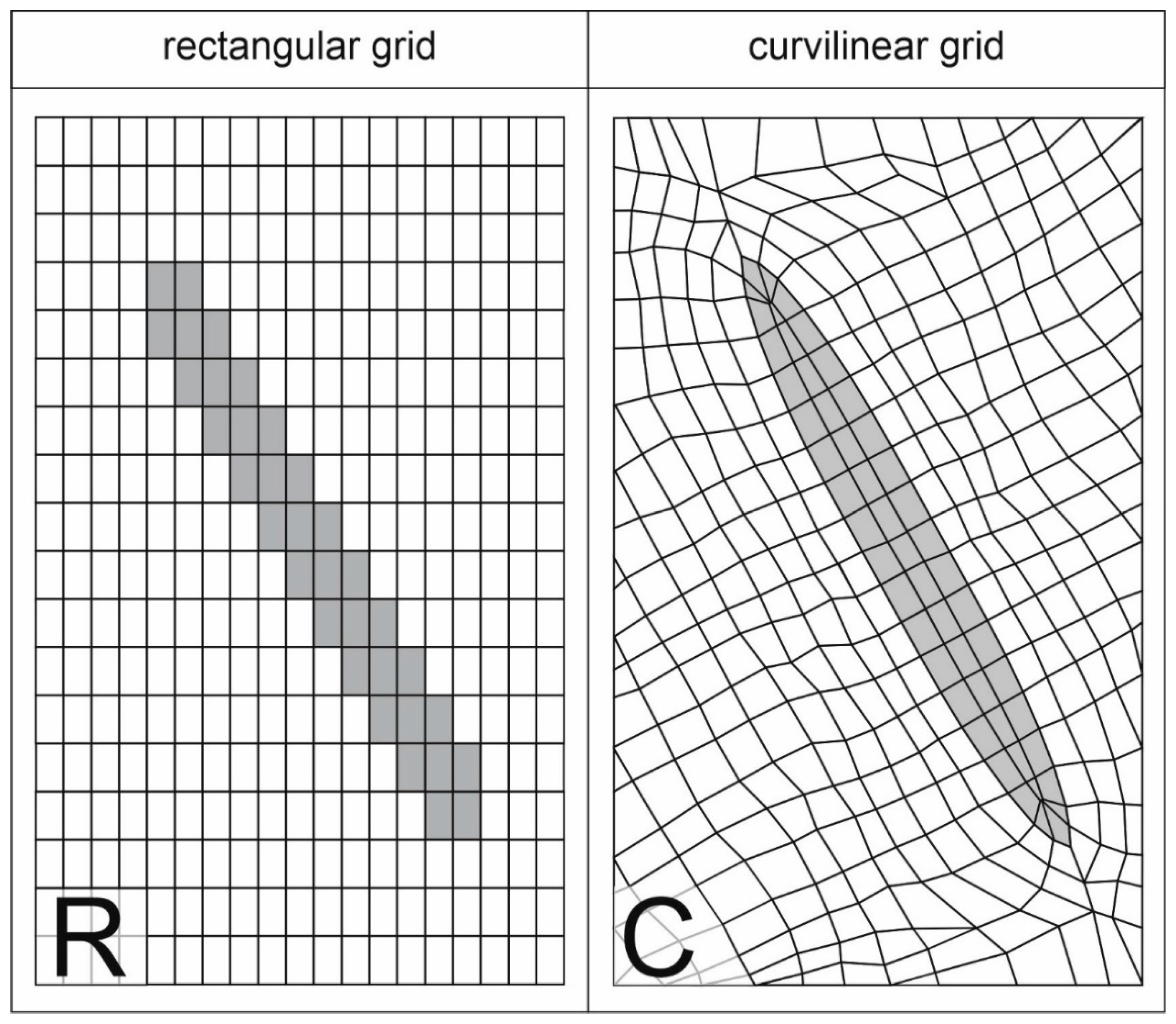
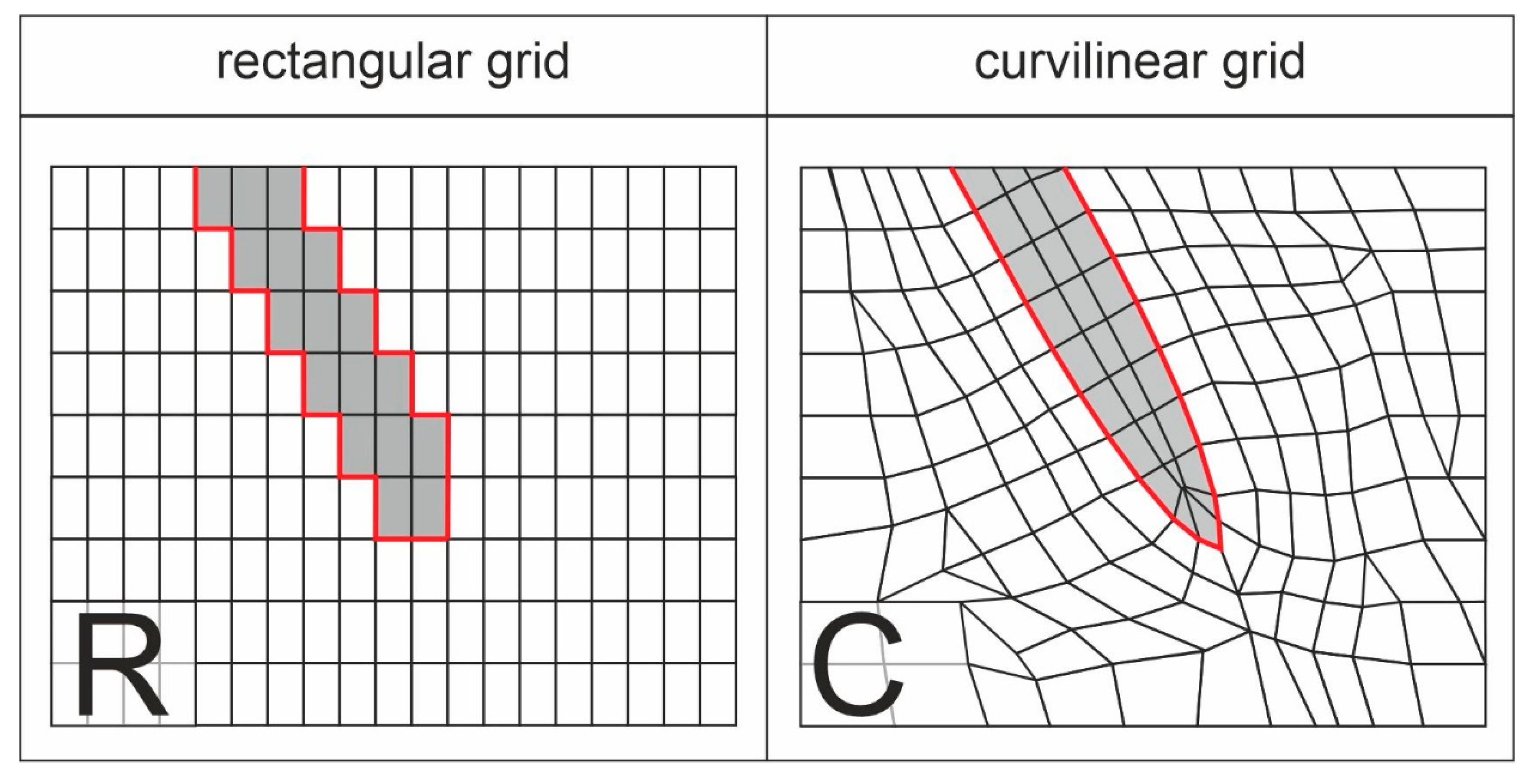
3.2. Grid Geometry
3.2.1. Rectangular Approach
3.2.2. Curvilinear Approach
3.3. Fault Dip
4. Model Setup
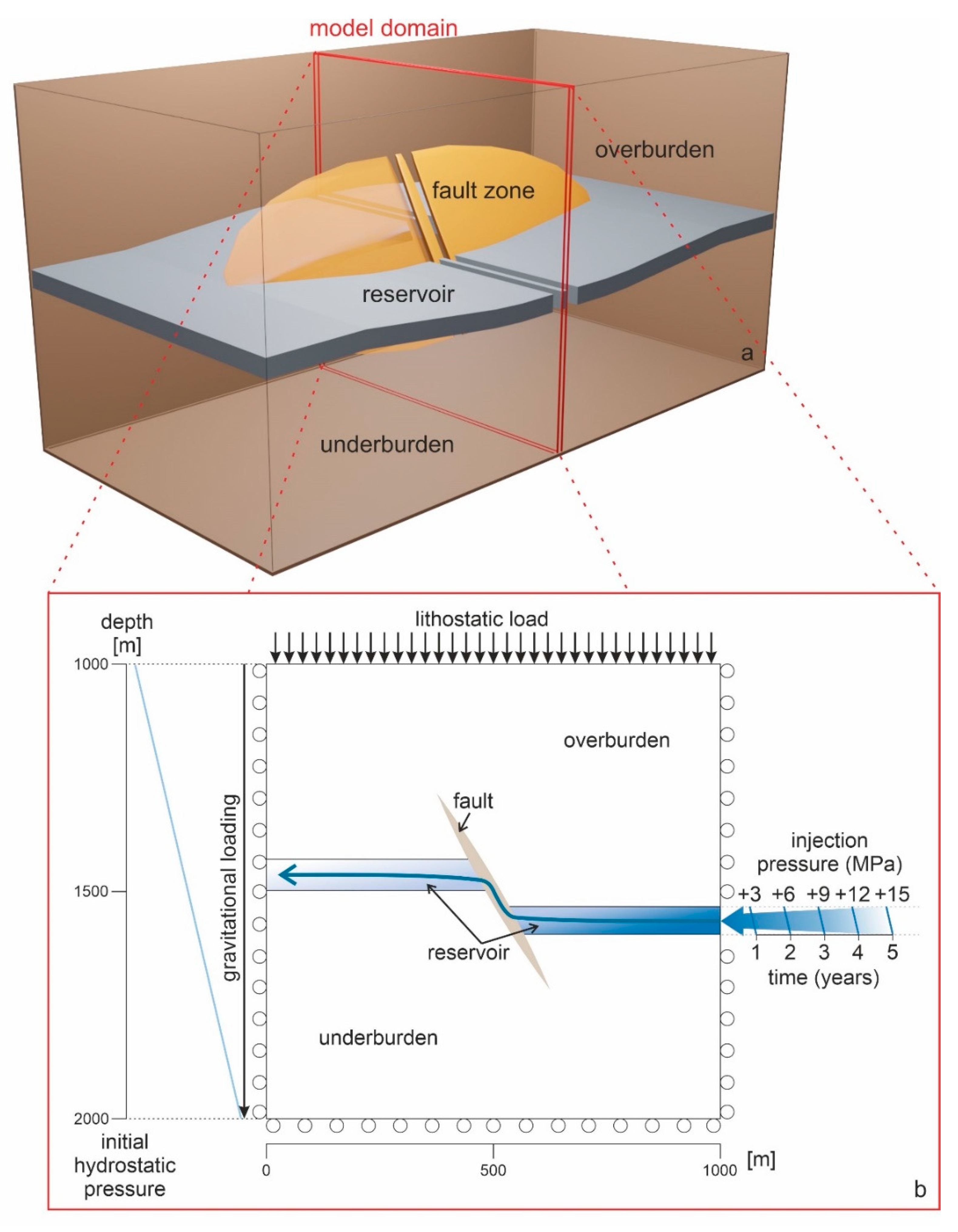
4.1. Model Geometry
4.2. Boundary Conditions
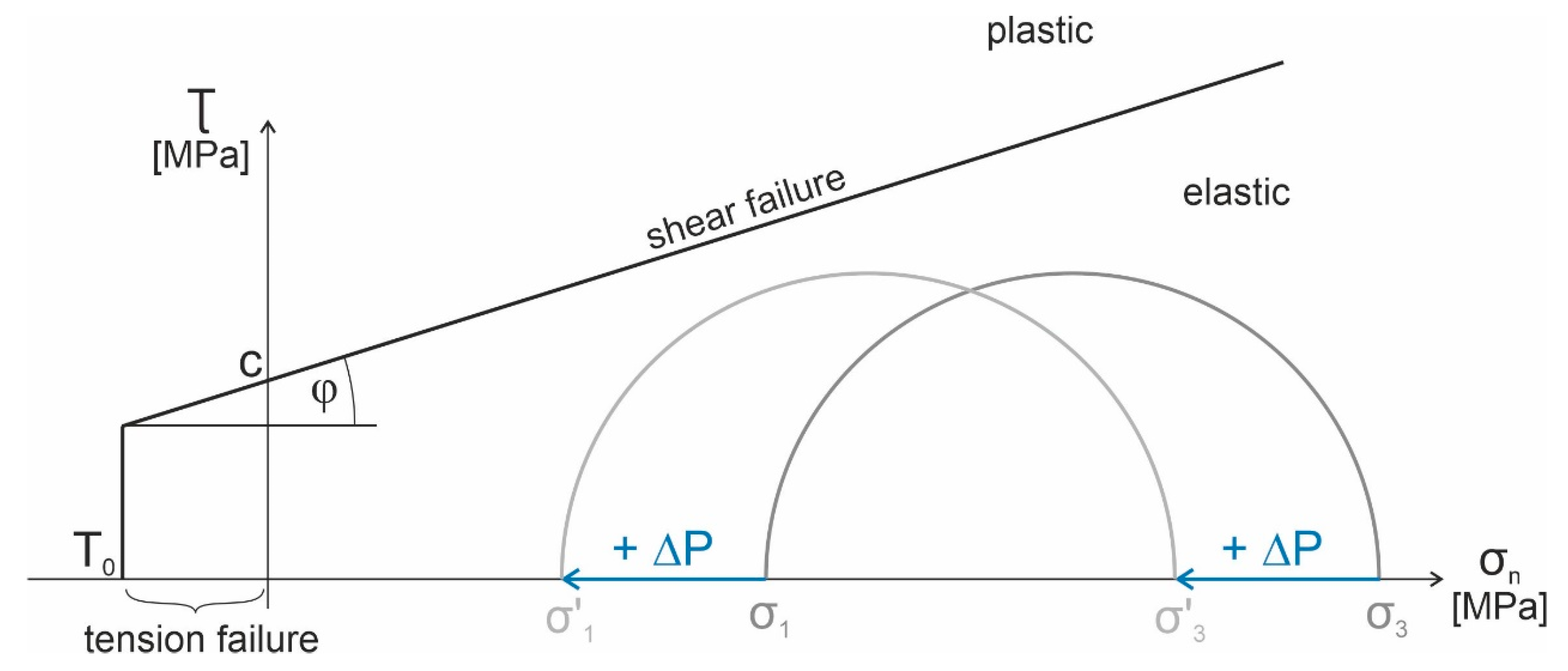
4.3. Constitutive Laws
4.4. Material Input Parameters
5. Results
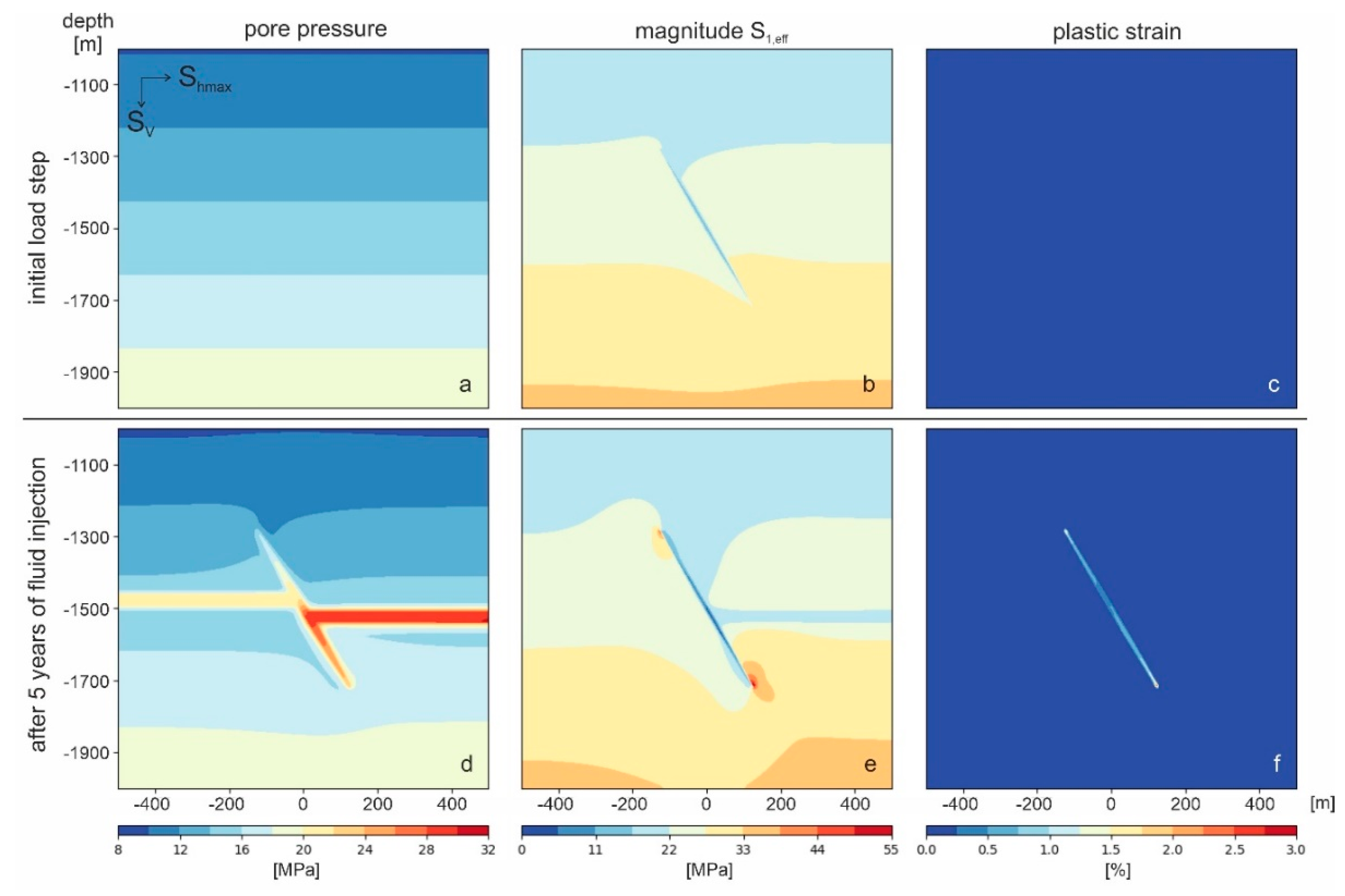
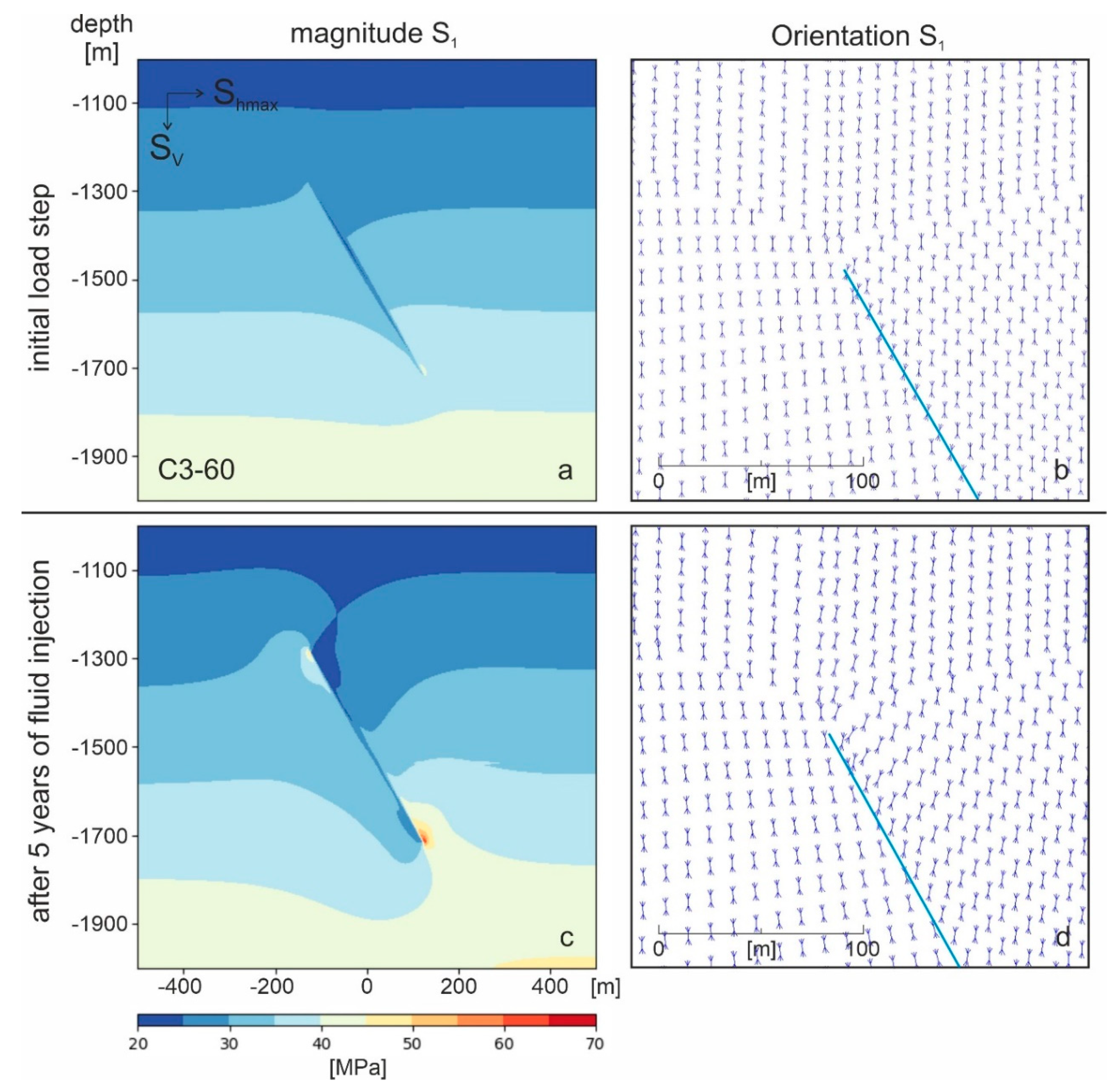
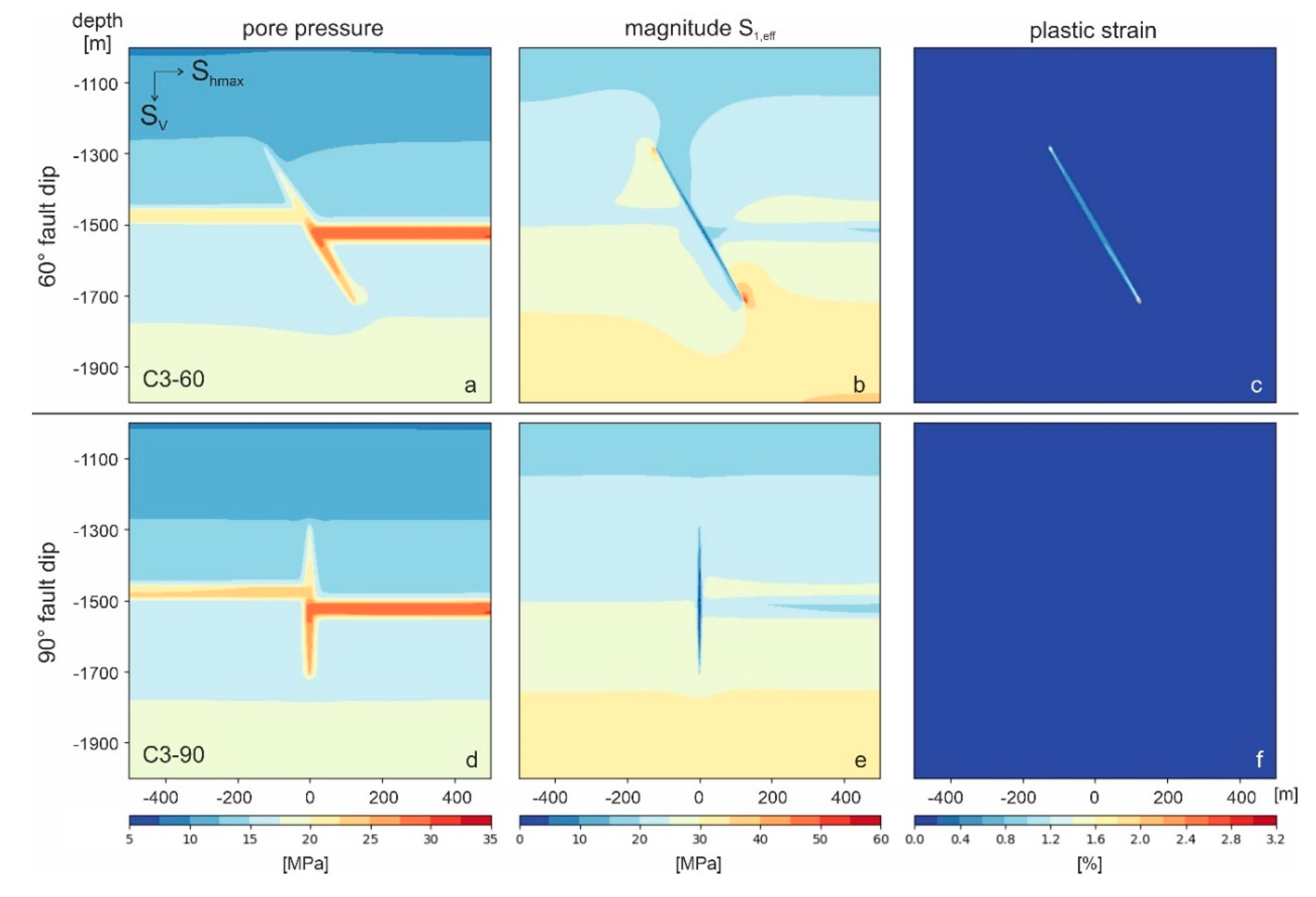
5.1. Reference Model (C3-60)
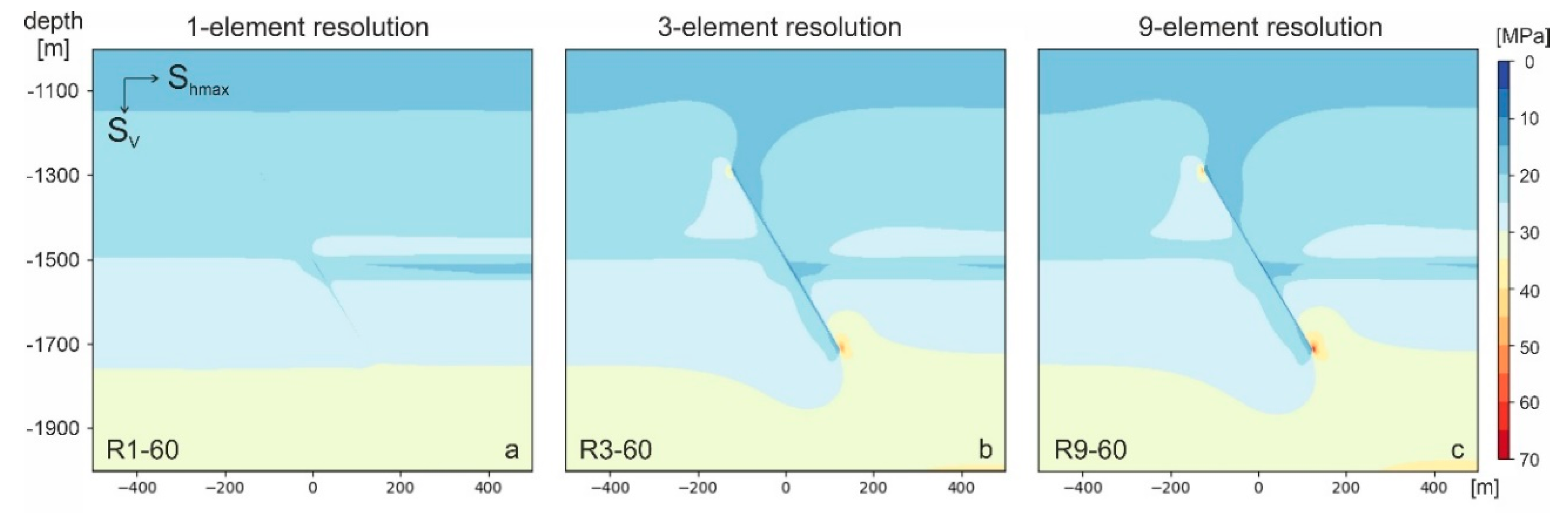
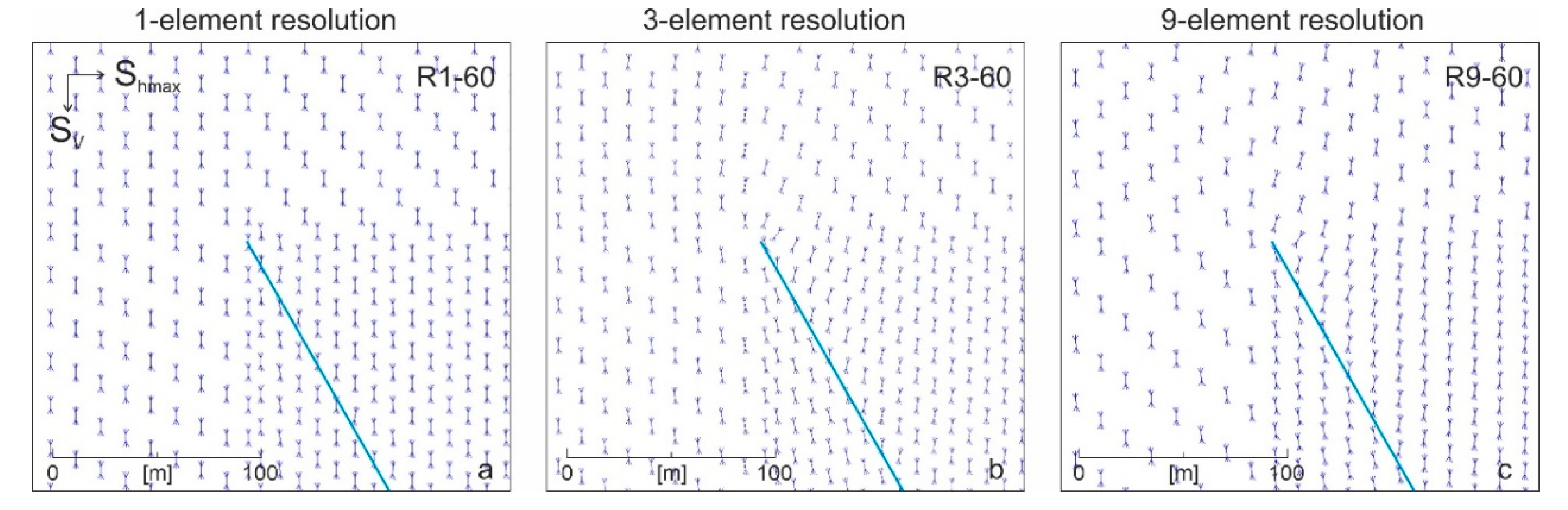
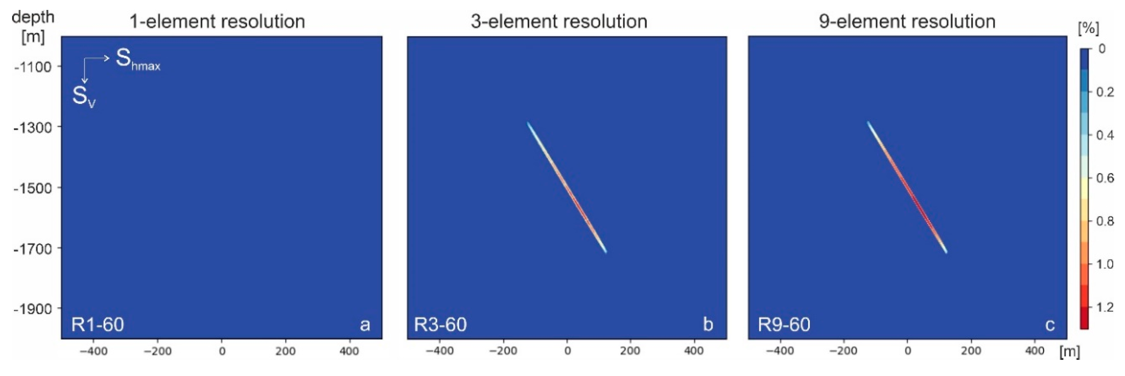
5.2. Mesh Resolution
5.3. Grid Geometry
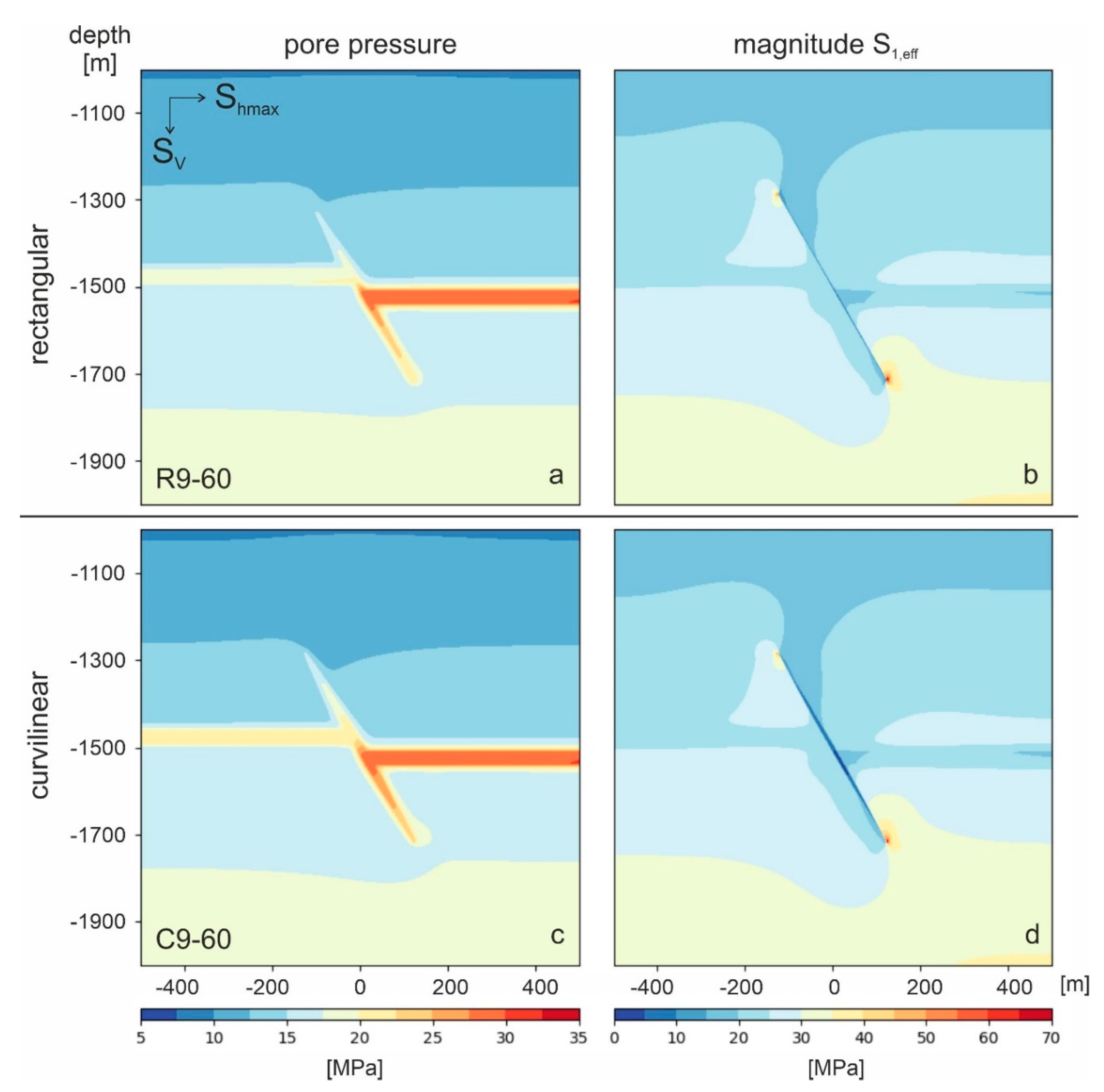
5.3.1. Pore Pressure and Effective Stress Magnitude
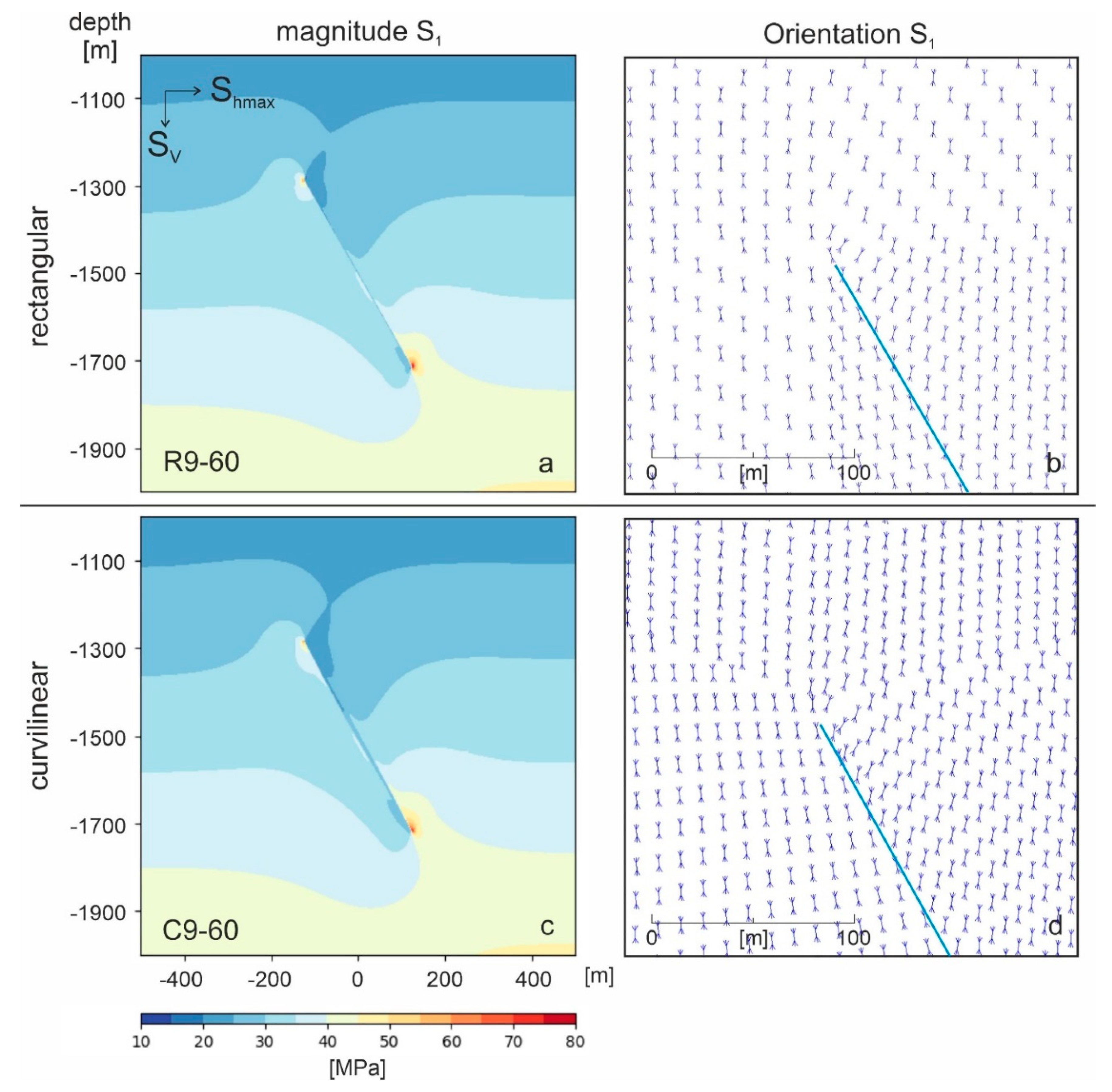
5.3.2. Stress Orientation
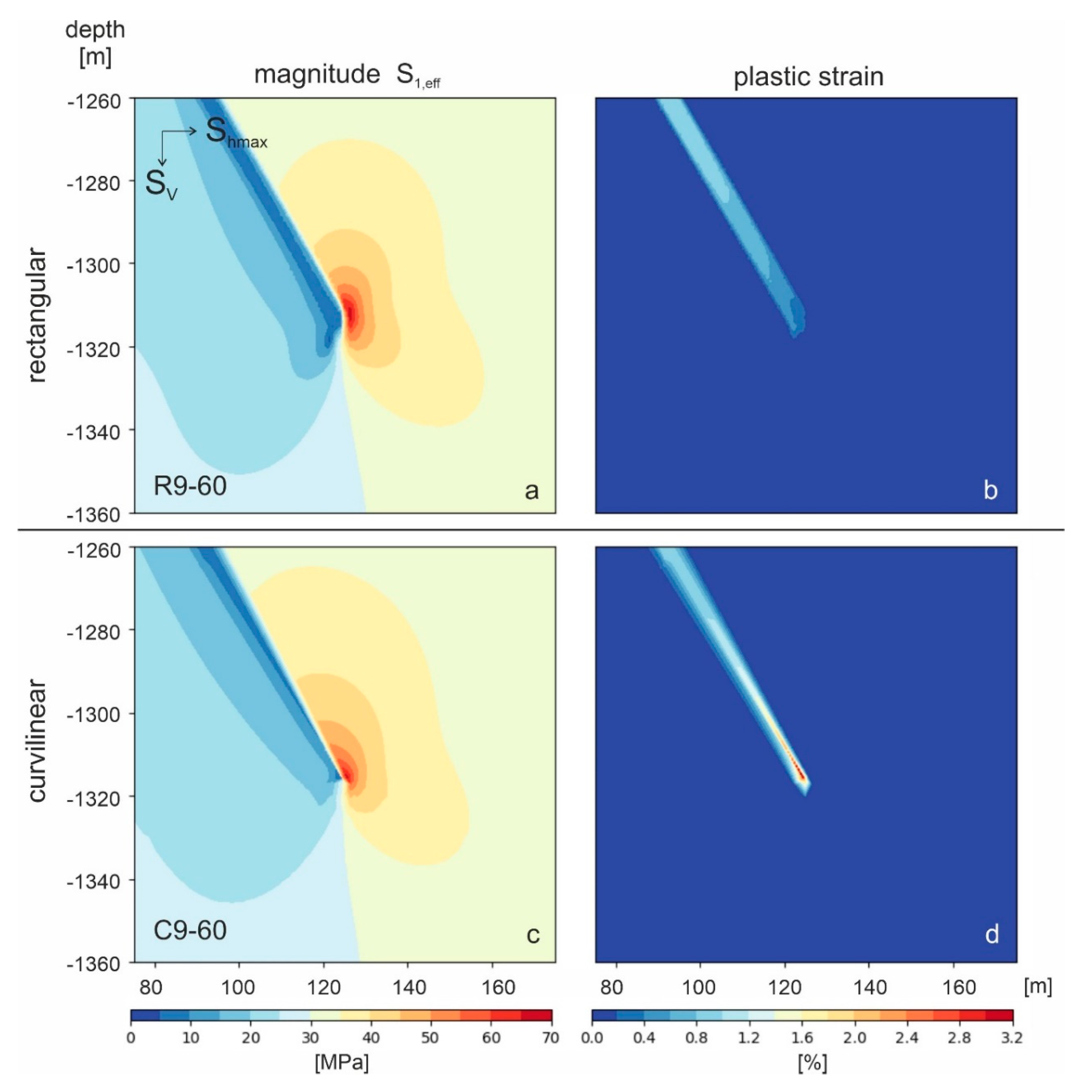
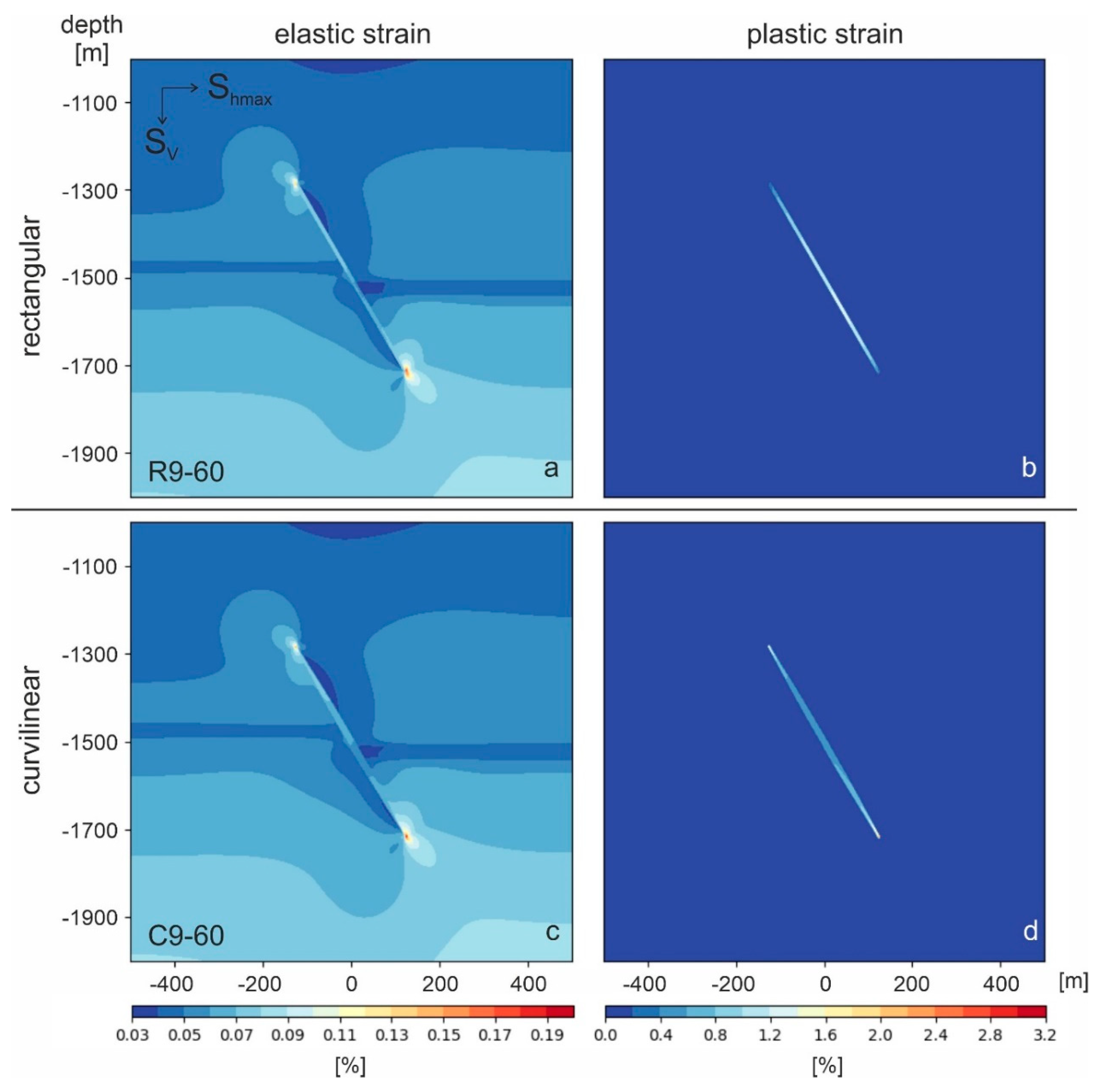
5.3.3. Elastic and Plastic Strain
5.4. Fault Dip
6. Discussion
6.1. Mesh Resolution
6.2. Grid Geometry
6.3. Fault Dip
6.4. Practical Aspects of Model Building
7. Conclusions
- The mesh resolution has to be considered very carefully, since it can—combined with a rectangular grid—lead to serious errors. It needs to be ensured that the fault cells do not interlock with the surrounding, stronger and less permeable host rock as this effects both fluid flow through and straining of the fault zone. This interlocking effect mainly occurs for 1-element width fault zones. For grids with multiple element wide fault zones, the only differences are observed in the vicinity of the fault tips. Three element wide fault zones appear to be appropriate for most reservoir-scale models. Only if the aim of the study is within 10 m of the fault zone, a finer resolution should be considered.
- If the aim of the study is to model the fault zone properly, a curvilinear representation is recommended. In addition to somewhat better fluid migration throughout the whole fault zone, this approach shows higher plastic strain at the fault tips, which appears to be closer to reality.
- If the aim of the study is at a distance of more than 10 m from the fault, both grid geometries are interchangeable. They show similar stress and strain patterns. In this case, the advantage of the rectangular grid is that it generally takes much less time to generate.
- Different fault dips produce different mechanical results, i.e., stress and strain patterns. Therefore, care should be taken to consider a realistic fault dip, e.g., from interpretation of depth-converted seismic sections, rather than using a vertical fault dip for simplification.
- Different fault dips produce similar hydraulic results. If the aim of the study is primarily on hydraulic issues, vertical faults can be an acceptable simplification.
Author Contributions
Funding
Acknowledgments
Conflicts of Interest
References
- Pereira, L.C.; Guimarães, L.J.N.; Horowitz, B.; Sánchez, M. Coupled hydromechanical fault reactivation analysis incorporating evidence theory for uncertainty quantification. Comput. Geotech. 2014, 56, 202–215. [Google Scholar] [CrossRef]
- Rueda, J.C.; Norena, N.V.; Oliveira, M.F.F.; Roehl, D. Numerical Models for Detection of Fault Reactivation in Oil and Gas Fields. In Proceedings of the 48th US Rock Mechanics/Geomechanics Symposium, Minneapolis, MN, USA, 1–4 June 2014. [Google Scholar]
- Fachri, J.T.M.; Røe, P. Volumetric faults in field-sized reservoir simulation models: A first case study. AAPG Bull. 2016, 100, 795–817. [Google Scholar] [CrossRef]
- Manzocchi, T.; Heath, A.E.; Palananthakumar, B.; Childs, C.; Walsh, J. Faults in conventional flow simulation models: A consideration of representational assumptions and geological uncertainties. Pet. Geosci. 2008, 14, 91–110. [Google Scholar] [CrossRef]
- Qu, D.; Røe, P.; Tveranger, J. A method for generating volumetric fault zone grids for pillar gridded reservoir models. Comput. Geosci. 2015, 81, 28–37. [Google Scholar] [CrossRef] [Green Version]
- Segall, P.; Grasso, J.-R.; Mossop, A. Poroelastic stressing and induced seismicity near the Lacq gas field, southwestern France. J. Geophys. Res. Space Phys. 1994, 99, 15423. [Google Scholar] [CrossRef]
- Geertsma, J. Land subsidence abovec ompacting oil and gas reservoirs. J. Pet. Technol. 1973, 5, 734–744. [Google Scholar] [CrossRef]
- Fisher, Q.J.; Jolley, S.J. Treatment of faults in production simulation models. In Structurally Complex Reservoirs; Jolley, S.J., Barr, D., Walsh, J.J., Knipe, R.J., Eds.; Geological Society—Special Publications: London, UK, 2007; Volume 292, pp. 219–233. [Google Scholar]
- Ferronato, M.; Janna, C.; Gambolati, G. Mixed constraint preconditioning in computational contact mechanics. Comput. Methods Appl. Mech. Eng. 2008, 197, 3922–3931. [Google Scholar] [CrossRef]
- Orlić, B.; Wassing, B.B.T. A Study of Stress Change and Fault Slip in Producing Gas Reservoirs Overlain by Elastic and Viscoelastic Caprocks. Rock Mech. Rock Eng. 2012, 46, 421–435. [Google Scholar] [CrossRef]
- Cappa, F.; Rutqvist, J. Modeling of coupled deformation and permeability evolution during fault reactivation induced by deep underground injection of CO2. Int. J. Greenh. Gas Control. 2011, 5, 336–346. [Google Scholar] [CrossRef] [Green Version]
- Zhang, Y.; Langhi, L.; Schaubs, P.; Piane, C.D.; Dewhurst, D.; Stalker, L.; Michael, K. Geomechanical stability of CO2 containment at the South West Hub Western Australia: A coupled geomechanical–fluid flow modelling approach. Int. J. Greenh. Gas Control. 2015, 37, 12–23. [Google Scholar] [CrossRef]
- Jing, L.; Hudson, J. Numerical methods in rock mechanics. Int. J. Rock Mech. Min. Sci. 2002, 39, 409–427. [Google Scholar] [CrossRef]
- Hilley, G.E.; Mynatt, I.; Pollard, D. Structural geometry of Raplee Ridge monocline and thrust fault imaged using inverse Boundary Element Modeling and ALSM data. J. Struct. Geol. 2010, 32, 45–58. [Google Scholar] [CrossRef]
- Fournier, T.; Morgan, J. Insights to slip behavior on rough faults using discrete element modeling. Geophys. Res. Lett. 2012, 39, 1–6. [Google Scholar] [CrossRef] [Green Version]
- Crocher, A.; O’Sullivan, M. Application of the computer code TOUGH2 tot the simulation of supercritical conditions in geothermal systems. Geothermics 2008, 37, 622–634. [Google Scholar] [CrossRef]
- Jayakumar, R.; Sahai, V.; Boulis, A. A Better Understanding of Finite Element Simulation for Shale Gas Reservoirs through a Series of Different Case Histories. In Proceedings of the SPE Middle East Unconventional Gas Conference and Exhibition, Muscat, Oman, 31 January–2 February 2011; Society of Petroleum Engineers: Richardson, TX, USA, 2011; pp. 245–262. [Google Scholar]
- Nasir, O.; Fall, M.; Nguyen, T.S.; Evgin, E. Modeling of the thermohydromechanical–chemical response of Ontario sedimentary rocks to future glaciations. Can. Geotech. J. 2015, 52, 836–850. [Google Scholar] [CrossRef]
- Yale, D.P. Fault and stress magnitude controls on variations in the orientation of in situ stress. In Fracture and In-Situ Stress Characterization of Hydrocarbon Reservoirs; Ameen, M., Ed.; Geological Society—Special Publications: London, UK, 2003; Volume 209, pp. 55–64. [Google Scholar]
- Fredman, N.; Tveranger, J.; Cardozo, N.; Braathen, A.; Soleng, H.; Røe, P.; Skorstad, A.; Syversveen, A.R. Fault facies modeling: Technique and approach for 3-D conditioning and modeling of faulted grids. AAPG Bull. 2008, 92, 1457–1478. [Google Scholar] [CrossRef]
- Faulkner, D.; Jackson, C.; Lunn, R.J.; Schlische, R.; Shipton, Z.K.; Wibberley, C.; Withjack, M. A review of recent developments concerning the structure, mechanics and fluid flow properties of fault zones. J. Struct. Geol. 2010, 32, 1557–1575. [Google Scholar] [CrossRef]
- Morton, R.; Bernier, J.; Barras, J.A. Evidence of regional subsidence and associated interior wetland loss induced by hydrocarbon production, Gulf Coast region, USA. Environ. Earth Sci. 2006, 50, 261–274. [Google Scholar] [CrossRef]
- Chan, A.W.; Zoback, M.D. The role of hydrocarbon production on land subsidence and fault reactivation in the Loiusiana Coastal Zone. J. Coast. Res. 2007, 24, 771–786. [Google Scholar] [CrossRef]
- Fredman, N.; Tveranger, J.; Semshaug, S.; Braathen, A.; Sverdrup, E. Sensitivity of fluid flow to fault core architecture and petrophysical properties of fault rocks in siliciclastic reservoirs: A synthetic fault model study. Pet. Geosci. 2007, 13, 305–320. [Google Scholar] [CrossRef]
- Braathen, A.; Tveranger, J.; Fossen, H.; Skar, T.; Cardozo, N.; Semshaug, S.E.; Bastesen, E.; Sverdrup, E. Fault facies and its application to sandstone reservoirs. AAPG Bull. 2009, 93, 891–917. [Google Scholar] [CrossRef] [Green Version]
- Fachri, M.; Rotevatn, A.; Tveranger, J. Fluid flow in relay zones revisited: Towards an improved representation of small-scale structural heterogeneities in flow models. Mar. Pet. Geol. 2013, 46, 144–164. [Google Scholar] [CrossRef]
- Qu, D.; Tveranger, J. Incorporation of deformation band fault damage zones in reservoir models. AAPG Bull. 2016, 100, 423–443. [Google Scholar] [CrossRef] [Green Version]
- Fischer, K.; Henk, A. A workflow for building and calibrating 3-D geomechanical models—A case study for a gas reservoir in the North German Basin. Solid Earth 2013, 4, 1–9. [Google Scholar] [CrossRef] [Green Version]
- De Souza, A.L.S.; De Souza, J.A.B.; Meurer, G.B.; Naveira, V.P.; Chaves, R.A.P. Reservoir Reomechanics Study for Deepwater Field Identifies Ways to Maximize Reservoir Performance while Reducing Geomechanics Risk. In Proceedings of the SPE Asia Pacific Oil and Gas Conference, Perth, Australia, 22–24 October 2012. [Google Scholar]
- Knai, T.A.; Knipe, R.J. The impact of faults on fluid flow in the Heidrun Field. In Faulting, Fault Sealing and Fluid Flow in Hydrocarbon Reservoirs; Jones, G., Fisher, Q.J., Knipe, R.J., Eds.; Geological Society—Special Publications: London, UK, 1998; Volume 147, pp. 269–282. [Google Scholar]
- Walsh, J.; Watterson, J.; Heath, A.E.; Childs, C. Representation and scaling of faults in fluid flow models. Pet. Geosci. 1998, 4, 241–251. [Google Scholar] [CrossRef]
- Hollund, K.; Mostad, P.; Nielsen, B.F. Havana—A fault modelling tool. In Hydrocarbon Seal Quantification; Koestler, A.G., Hunsdale, R., Eds.; Norwegian Petroleum Society—Special Publications: Oslo, Norway, 2002; Volume 11, pp. 157–171. [Google Scholar]
- Jolley, S.J.; Dijk, H.; Lamens, J.H.; Fisher, Q.J.; Manzocchi, T.; Eikmans, H.; Huang, Y. Faulting and fault sealing in production simulation models: Brent Province, northern North Sea. Pet. Geosci. 2007, 13, 321–340. [Google Scholar] [CrossRef] [Green Version]
- Manzocchi, T.; Walsh, J.; Nell, P.; Yielding, G. Fault transmissibility multipliers for flow simulation models. Pet. Geosci. 1999, 5, 53–63. [Google Scholar] [CrossRef]
- Crawford, B.R.; Myers, R.D.; Woronow, A.; Faulkner, D.R.; Rutter, E.H. Porosity–permeability relationships in clay-bearing fault gouge. In Proceedings of the Society of Petroleum Engineers/International Society of Rock Mechanics Conference, Iving, TX, USA, 20–23 October 2002. [Google Scholar]
- Myers, R.D.; Allgood, A.; Hjellbakk, A.; Vrolijk, P.; Briedis, N. Testing fault transmissibility predictions in a structurally dominated reservoir: Ringhorne Field, Norway. In Structurally Complex Reservoirs; Jolley, S.J., Barr, D., Walsh, J.J., Knipe, R.J., Eds.; Geological Society—Special Publications: London, UK, 2007; Volume 292, pp. 271–294. [Google Scholar]
- Tveranger, J.; Aanonsen, S.; Braathen, A.; Espedal, M.; Fossen, H.; Hesthammer, J.; Howell, J.; Pettersen, Ø.; Skorstad, A.; Skar, T.; et al. The Fault Facies Project. In Proceedings of the Production Geoscience, Stavanger, Norway, 29–30 May 2004. [Google Scholar]
- Byerlee, J. Friction of rocks. Pageoph 1978, 116, 615–626. [Google Scholar] [CrossRef]
- Wibberley, C.; Yielding, G.; DiToro, G. Recent advances in the understanding of fault zone internal structure: A review. In The Internal Structure of Fault Zones: Implications for Mechanical and Fluid-Flow Properties; Wibberley, C., Kurz, W., Imber, J., Holdsworth, R.E., Collettini, C., Eds.; Geological Society—Special Publications: London, UK, 2008; Volume 299, pp. 5–33. [Google Scholar]
- Barton, N. Shear strength criteria for rock, rock joints, rockfill and rock masses: Problems and some solutions. J. Rock Mech. Geotech. Eng. 2013, 5, 249–261. [Google Scholar] [CrossRef] [Green Version]
- Hergert, T.; Heidbach, O.; Bécel, A.; Laigle, M. Geomechanical model of the Marmara Sea region-I. 3-D contemporary kinematics. Geophys. J. Int. 2011, 185, 1073–1089. [Google Scholar] [CrossRef]
- Franceschini, A.; Ferronato, M.; Janna, C.; Teatini, P. A novel Lagrangian approach for the stable numerical simulation of fault and fracture mechanics. J. Comput. Phys. 2016, 314, 503–521. [Google Scholar] [CrossRef]
- Rinaldi, A.P.; Jeanne, P.; Rutqvist, J.; Cappa, F. Geomechanical effects during large-scale underground injection. In Proceedings of the 47th US Rock Mechanics—Geomechanics Symposium, San Francisco, CA, USA, 23–26 June 2013. [Google Scholar]
- Vilarrasa, V.; Makhnenko, R.Y.; Laloui, L. Potential for Fault Reactivation Due to CO2 Injection in a Semi-Closed Saline Aquifer. Energy Procedia 2017, 114, 3282–3290. [Google Scholar] [CrossRef] [Green Version]
- Treffeisen, T.; Henk, A. Representation of faults in reservoir-scale geomechanical finite element models—A comparison of different modelling approaches. J. Struct. Geol. 2020, 131, 1–12. [Google Scholar] [CrossRef]
- Buchmann, T.J.; Connolly, P.T. Contemporary kinematics of the Upper Rhine Graben: A 3D finite element approach. Glob. Planet. Chang. 2007, 58, 287–309. [Google Scholar] [CrossRef]
- Ye, S.; Franceschini, A.; Zhang, Y.; Janna, C.; Gong, X.; Yu, J.; Teatini, P. A Novel Approach to Model Earth Fissure Caused by Extensive Aquifer Exploitation and its Application to the Wuxi Case, China. Water Resour. Res. 2018, 54, 2249–2269. [Google Scholar] [CrossRef]
- Prevost, J.H.; Sukumar, N. Faults simulations for three-dimensional reservoir-geomechanical models with the extended finite element method. J. Mech. Phys. Solids 2016, 86, 1–18. [Google Scholar] [CrossRef]
- Deb, R.; Jenny, P. Modeling of shear failure in fractured reservoirs with a porous matrix. Comput. Geosci. 2017, 21, 1119–1134. [Google Scholar] [CrossRef]
- Will, J.; Eckardt, S. optiRiss—Simulation-based optimization and risk evaluation of enhanced geothermal systems. In Proceedings of the 12 Weimarer Optimierungs und Stochastiktage, Weimar, Germany, 5–6 November 2015. [Google Scholar]
- Schlegel, R. Neue Geomechanische Materialmodelle. CADFEM J. 2016, 1, 24–25. [Google Scholar]
- Syversveen, A.; Skorstad, A.; Soleng, H.; Røe, P.; Tveranger, J. Facies modelling in fault zones. In Proceedings of the 10th European Conference on the Mathematics of Oil Recovery, Amsterdam, The Netherlands, 4–7 September 2006. [Google Scholar]
- Sanchez, E.C.; Zegarra, E.; Oliveira, M.F.F.; Roehl, D. Application of a 2D equivalent continuum approach to the assessment of geological fault reactivation in reservoirs. In Proceedings of the XXXVI Ibero-Latin American Congress on Computational Methods in Engineering, Rio de Janeiro, Brazil, 22–25 November 2015. [Google Scholar]
- Schuite, J.; Longuevergne, L.; Bour, O.; Burbey, T.J.; Boudin, F.; Lavenant, N.; Davy, P. Understanding the Hydromechanical Behavior of a Fault Zone From Transient Surface Tilt and Fluid Pressure Observations at Hourly Time Scales. Water Resour. Res. 2017, 53, 10558–10582. [Google Scholar] [CrossRef] [Green Version]
- Ghavidel, A.; Mousavi, S.R.; Rashki, M. The Effect of FEM Mesh Density on the Failure Probability Analysis of Structures. KSCE J. Civ. Eng. 2017, 22, 2370–2383. [Google Scholar] [CrossRef]
- Azarfar, B.; Peik, B.; Abbasi, B. A Discussion on Numerical Modeling of Fault for Large Open Pit Mines. In Proceedings of the 52th US Rock Mechanics/Geomechanics Symposium, Seattle, WA, USA, 17–20 June 2018. [Google Scholar]
- Knupp, P.M. Mesh quality improvement for SciDAC applications. J. Phys. Conf. Ser. 2006, 46, 458–462. [Google Scholar] [CrossRef]
- Henk, A. Numerical Modelling of Faults. In Understanding Faults—Detecting, Dating and Modeling, 1st ed.; Tanner, D., Brandes, C., Eds.; Elsevier: Amsterdam, The Netherlands, 2019; pp. 147–164. [Google Scholar]
- Olden, P.; Pickup, G.E.; Jin, M.; Mackay, E.J.; Hamilton, S.; Somerville, J.; Todd, A. Use of rock mechanics laboratory data in geomechanical modelling to increase confidence in CO2 geological storage. Int. J. Greenh. Gas Control. 2012, 11, 304–315. [Google Scholar] [CrossRef]
- De Souza, A.L.S.; De Souza, J.A.B.; Meurer, G.B.; Chaves, R.A.P.; Frydman, M.; Pastor, J. Integrated 3D geomechanics and reservoir simulation optimize performance avoid fault reactivation. World Oil 2014, 4, 55–58. [Google Scholar]
- Rippon, J.H. Contoured patterns of the throw and hade of normal faults in the Coal Measures (Westphalian) of northwest Derbyshire. Proc. Yorks. Geol. Soc. 1985, 45, 147–161. [Google Scholar] [CrossRef]
- Cowie, P.A.; Scholz, C.H. Displacement-length scaling relationship for faults: Data synthesis and discussion. J. Struct. Geol. 1992, 14, 1149–1156. [Google Scholar] [CrossRef]
- Chopra, S.; Marfurt, K. Seismic Attributes for Prospect Identification and Reservoir Characterization, 1st ed.; SEG Geophysical Developments 11: Tulsa, OK, USA, 2007. [Google Scholar]
- Couples, G.; Ma, J.; Lewis, H.; Olden, P.; Quijano, J.; Fasae, T.; Maguire, R. Geomechanics of faults: Impacts on seismic imaging. First Break 2007, 25, 83–90. [Google Scholar]
- Tanner, D.C.; Buness, H.; Igel, J.; Günther, T.; Gabriel, G.; Skiba, P.; Plenefisch, T.; Gestermann, N.; Walter, T.R. Fault detection. In Understanding Faults—Detecting, Dating and Modeling, 1st ed.; Tanner, D., Brandes, C., Eds.; Elsevier: Amsterdam, The Netherlands, 2019; pp. 81–146. [Google Scholar]
- Geldart, L.P.; Sheriff, R.E. Exploration Seismology, 2nd ed.; Cambridge University Press: Cambridge, UK, 1995. [Google Scholar]
- Buske, S.; Gutjahr, S.; Sick, C. Fresnel volume migration of single-component seismic data. Geophysics 2009, 74, 47–55. [Google Scholar] [CrossRef]
- Liu, E.; Martinez, A. Seismic Fracture Characterization, Concepts and Practical Applications. In Proceedings of the EAGE, Copenhagen, The Netherlands, 4–7 June 2012. [Google Scholar]
- Moser, T.J.; Howard, C. Diffraction imaging in depth. Geophys. Prospect. 2008, 56, 627–641. [Google Scholar] [CrossRef]
- Ghose, R.; Carvalho, J.; Loureiro, A. Signature of fault zone deformation in near-surface soil visible in shear wave seismic reflections. Geophys. Res. Lett. 2013, 40, 1074–1078. [Google Scholar] [CrossRef] [Green Version]
- Baysal, E.; Kosloff, D.; Sherwood, J.W.C. Reverse time migration. Geophysics 1983, 48, 1514–1524. [Google Scholar] [CrossRef] [Green Version]
- Jones, I.F.; Ibbotson, K.; Grimshaw, M.; Plasterie, P. 3-D prestack depth migration and velocity model building. Geophysics 1998, 17, 897–906. [Google Scholar]
- Anderson, E.M. The Dynamics of Faulting and Dyke Formation with Application to Britain, 2nd ed.; Oliver and Boyd: Edinburgh, UK, 1951. [Google Scholar]
- Ansys 19.2; Ansys Inc.: Canonsburg, PA, USA, 2019.
- Johri, M.; Zoback, M.D.; Hennings, P. A scaling law to characterize fault-damage zones at reservoir depths. AAPG Bull. 2014, 98, 2057–2079. [Google Scholar] [CrossRef] [Green Version]
- Jaeger, J.; Cook, N.G.; Zimmerman, R. Fundamentals of Rock Mechanics, 4th ed.; Wiley-Blackwell: Oxford, UK, 2007. [Google Scholar]
- Wang, H.F. Theory of Linear Poroelasticity—With Applications to Geomechanics and Hydrogeology; Princeton University Press: Princeton, NJ, USA; Oxford, UK, 2000. [Google Scholar]
- Shapiro, S. Fundamentals of poroelasticity. In Fluid-Induced Seismicity; Shapiro, S., Ed.; Cambridge University Press: Cambridge, UK, 2015; pp. 48–117. [Google Scholar]
- Cheng, A.H.D. Poroelasticity; Springer International Publishing: Basel, Switzerland, 2016. [Google Scholar]
- Streit, J.E.; Hillis, R.R. Estimating fault stability and sustainable fluid pressures for underground storage of CO2 in porous rock. Energy 2004, 29, 1445–1456. [Google Scholar] [CrossRef]
- Holdsworth, R.E. Weak faults—Rotten cores. Science 2004, 303, 181–182. [Google Scholar] [CrossRef]
- Faulkner, D. A model for the variation in permeability of clay-bearing fault gouge with depth in the brittle crust. Geophys. Res. Lett. 2004, 31, 1–5. [Google Scholar] [CrossRef]
- Collettini, C.; Niemeijer, A.; Viti, C.; Marone, C. Fault zone fabric and fault weakness. Nature 2009, 462, 907–910. [Google Scholar] [CrossRef]
- Caine, J.S.; Evans, J.P.; Forster, C.B. Fault zone architecture and permeability structure. Geology 1996, 24, 1025. [Google Scholar] [CrossRef]
- Agosta, F.; Prasad, M.; Aydin, A. Physical properties of carbonate fault rocks, fucino basin (Central Italy): Implications for fault seal in platform carbonates. Geofluids 2007, 7, 19–32. [Google Scholar] [CrossRef]
- Cuisiat, F.; Jostad, H.P.; Andresen, L.; Skurtveit, E.; Skomedal, E.; Hettema, M.; Lyslo, K. Geomechanical integrity of sealing faults during depressurization of the Statfjord field. J. Struct. Geol. 2010, 32, 1754–1767. [Google Scholar] [CrossRef]
- Liu, Y. Choose the Best Element Size to Yield Accurate FEA Results While Reduce FE Models’s Complixity. Br. J. Eng. Technol. 2013, 1, 13–28. [Google Scholar]
- Ching, J.; Phoon, K.K. Effect of element sizes in random field finite element simulations of soil shear strength. Comput. Struct. 2013, 126, 120–134. [Google Scholar] [CrossRef]
- Ching, J.; Hu, Y.-G. Effect of Element Size in Random Finite Element Analysis for Effective Young’s Modulus. Math. Probl. Eng. 2016, 2016, 1–10. [Google Scholar] [CrossRef] [Green Version]
- Ashford, S.A.; Sitar, N. Effect of element size on the static finite element analysis of steep slopes. Int. J. Numer. Anal. Methods Géoméch. 2001, 25, 1361–1376. [Google Scholar] [CrossRef]
- Huang, J.; Griffiths, D. Determining an appropriate finite element size for modelling the strength of undrained random soils. Comput. Geotech. 2015, 69, 506–513. [Google Scholar] [CrossRef]
- Li, Y.; Wierzbicki, T. Mesh-size Effect Study of Ductile Fracture by Non-local Approach. In Proceedings of the SEM Annual Conference, Albuquerque, NM, USA, 1–4 June 2009. [Google Scholar]
- More, T.; Bindu, R.S. Effect of Mesh Size on Finite Element Analysis of Plate Structure. Int. J. Eng. Sci. Innov. Technol. 2015, 4, 1–5. [Google Scholar]
- Dutt, A. Lovely Professional University Effect of Mesh Size on Finite Element Analysis of Beam. Int. J. Mech. Eng. 2015, 2, 8–10. [Google Scholar] [CrossRef] [Green Version]
- Liu, Y.; Glass, G. Effects of Mesh Density on Finite Element Analysis. In Proceedings of the SAE World Congress, Detroit, MI, USA, 16–18 April 2013. [Google Scholar]
- Gudmundsson, A. Rock Fractures in Geological Processes; Cambridge University Press: Cambridge, UK, 2011. [Google Scholar]
- Dyskin, A.V.; Germanovich, L.N. A model of crack growth in micro cracked rock. Int. J. Rock Mech. 1993, 30, 813–820. [Google Scholar] [CrossRef]
- Reches, Z.; Lockner, D.A. Nucleation and growth of faults in brittle rocks. J. Geophys. Res. Space Phys. 1994, 99, 18159–18173. [Google Scholar] [CrossRef]
- Hoek, E.; Martin, C. Fracture initiation and propagation in intact rock—A review. J. Rock Mech. Geotech. Eng. 2014, 6, 287–300. [Google Scholar] [CrossRef] [Green Version]
- Brace, W.F. An extension of the Griffith theory of fracture to rocks. J. Geophys. Res. Space Phys. 1960, 65, 3477–3480. [Google Scholar] [CrossRef]
- Cowie, P.A.; Shipton, Z.K. Fault tip displacement gradients and process zone dimensions. J. Struct. Geol. 1998, 20, 983–997. [Google Scholar] [CrossRef]
- Brandes, C.; Tanner, D. Fault mechanics and earthquakes. In Understanding Faults—Detecting, Dating and Modeling, 1st ed.; Tanner, D., Brandes, C., Eds.; Elsevier: Amsterdam, The Netherlands, 2019; pp. 11–80. [Google Scholar]
- Lin, J.; Parmentier, E. Quasistatic propagation of a normal fault: A fracture mechanics model. J. Struct. Geol. 1988, 10, 249–262. [Google Scholar] [CrossRef]


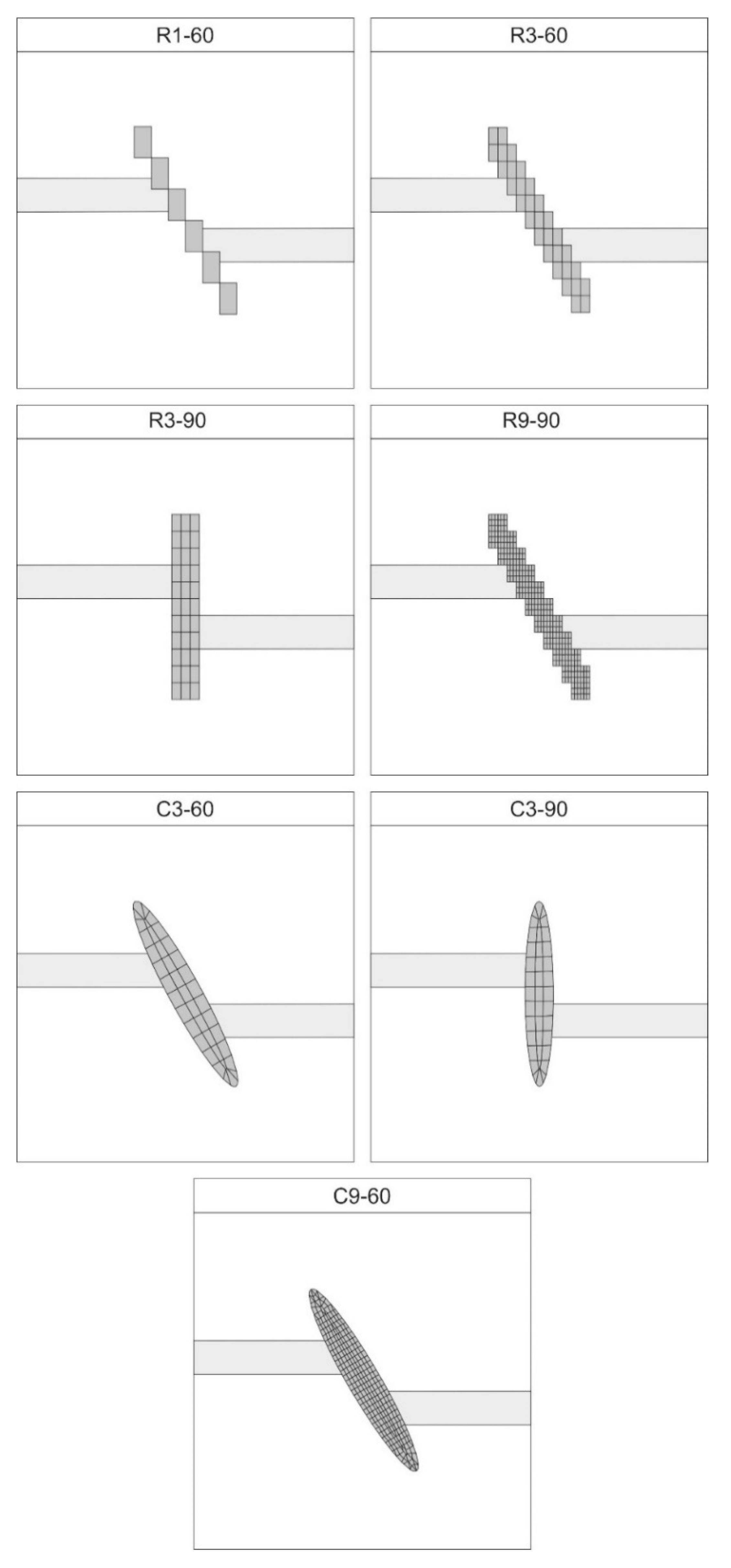
| Model Name | Grid Geometry | Fault Zone Width (Number of Elements) | Fault Dip (°) |
|---|---|---|---|
| R1-60 | rectangular | 1 | 60 |
| R3-60 | rectangular | 3 | 60 |
| R3-90 | rectangular | 3 | 90 |
| R9-60 | rectangular | 9 | 60 |
| C3-60 | curvilinear | 3 | 60 |
| C3-90 | curvilinear | 3 | 90 |
| C9-60 | curvilinear | 9 | 60 |
| Mechanical | Symbol | Fault Zone | Reservoir | Over-/Underburden |
|---|---|---|---|---|
| Young’s modulus (GPa) | E | 10 | 30 | 30 |
| Poisson’s’ ratio (–) | ν | 0.23 | 0.23 | 0.23 |
| Friction angle (°0) | φ | 10 | 40 | 40 |
| Cohesion (MPa) | c | 4 | 20 | 20 |
| Tensile strength (MPa) | TS | 5 | 20 | 20 |
| Density (kg/m3) | ρ | 2400 | 2400 | 2400 |
| Hydraulic | - | - | - | - |
| Biot coefficient (–) | A | 0.9 | 0.5 | 0.5 |
| Permeability (m2) | k | 10−14 | 5−12 | 10−17 |
| Porosity (–) | ϕ | 0.15 | 0.15 | 0.025 |
© 2020 by the authors. Licensee MDPI, Basel, Switzerland. This article is an open access article distributed under the terms and conditions of the Creative Commons Attribution (CC BY) license (http://creativecommons.org/licenses/by/4.0/).
Share and Cite
Treffeisen, T.; Henk, A. Faults as Volumetric Weak Zones in Reservoir-Scale Hydro-Mechanical Finite Element Models—A Comparison Based on Grid Geometry, Mesh Resolution and Fault Dip. Energies 2020, 13, 2673. https://doi.org/10.3390/en13102673
Treffeisen T, Henk A. Faults as Volumetric Weak Zones in Reservoir-Scale Hydro-Mechanical Finite Element Models—A Comparison Based on Grid Geometry, Mesh Resolution and Fault Dip. Energies. 2020; 13(10):2673. https://doi.org/10.3390/en13102673
Chicago/Turabian StyleTreffeisen, Torben, and Andreas Henk. 2020. "Faults as Volumetric Weak Zones in Reservoir-Scale Hydro-Mechanical Finite Element Models—A Comparison Based on Grid Geometry, Mesh Resolution and Fault Dip" Energies 13, no. 10: 2673. https://doi.org/10.3390/en13102673