Enhance of Energy Harvesting from Transverse Galloping by Actively Rotating the Galloping Body

Abstract

Kinematic rotary control is here proposed conceptually to enhance energy harvesting from Transverse Galloping. The effect of actively orientating the galloping body with respect to the incident flow, by imposing externally a rotation of the body proportional to the motion-induced angle of attack, is studied. To this end, a theoretical model is developed and analyzed, and numerical computations employing the Lattice Boltzmann Method are carried out. Good agreement is found between theoretical model predictions and numerical simulations results. It is found that it is possible to increase significantly the efficiency of energy harvesting with respect to the case without active rotation, which opens the path to consider this idea in practical realizations.

1. Introduction

During the last decade, the applied interest in the field of Flow-Induced vibrations has been enlarged by considering phenomena like Transverse Galloping or Vortex-induced Vibrations as the means to harvest useful energy from fluid flows. In those cases, the aim is to promote the Flow-Induced vibration phenomenon, in order to extract as much as possible part of the kinetic energy from the incoming flow and to transfer it to the body, in the form of mechanical oscillatory energy, and subsequently convert this mechanical energy into electrical energy by electromagnetic, piezoelectric, or electrostatic means. Bernitsas and his group of collaborators [1,2] proposed a system for electric power generation from marine/river currents taking advantage of the phenomenon of oscillations induced by vortex detachment in cylinders (Vortex-Induced Vibrations). Later on, in [3], the idea of taking advantage of the Transverse Galloping phenomenon was considered and, through analytical modeling, the role of the main parameters governing the problem, namely the geometry of the cross-section, mechanical parameters (mass, damping, stiffness) and flow velocity, was established and high energy transfer potential was proven. Since then, different concepts of energy extraction based on Transverse Galloping have appeared, with a focus on the large scale where a significant production of electric energy is desired [4], or to generate small amounts of electrical energy (of the order of milli-Watts) that can be used, for example, to supply electrical power to autonomous sensors and actuators and to avoid their dependence on batteries; see, for example, [5,6,7,8,9].

Very briefly, we can say that Transverse Galloping is a fluid-elastic instability that appears in some elastic bluff bodies when the velocity of the incident flow exceeds a critical value. Then, a small transverse displacement of the body induces an angle of attack relative to the incoming flow and a fluid force appears in the direction of the displacement in such a way that a net flux of energy from the fluid flow to the body appears and the later starts to oscillate transverse to the flow with increasing amplitude until a Limit Cycle of Oscillations is reached. Transverse Galloping is a self-induced phenomenon mainly driven by the motion-induced angle of attack (and not by vortex shedding like in Vortex-Induced Vibrations), which can only appear for specific cross-sections in which a variation of the motion-induced angle of attack produces a transverse fluid force in the direction of the velocity of oscillation. One notable difference of Transverse Galloping response compared to that of Vortex-Induced Vibrations is that, in the former, the amplitude of oscillations grows continuously with the incoming flow speed limit. For a detailed review of Transverse Galloping characteristics, the reader is referred to [10,11,12].

In a simplified manner, an energy-focused Transverse Galloping system is comprised of three main elements: (i) the galloping body, immersed in the fluid flow where the transverse fluid forces appear responsible for the transverse galloping phenomenon, (ii) the elastic system provides the restoring force and allows oscillations to happen, and (iii) a transducer, where the oscillatory mechanical power of the body is converted into electrical energy. The problem is fully coupled (double coupling fluid-solid-electrical), thus an integral perspective has to be taken into account in order to fully establish design rules to be able to harness energy efficiently. Some optimization studies in these three different elements have been carried out in the past: for example [3,13], looking for optimal cross-section geometry of the galloping body (let us say, looking for optimization on the “fluid side”); Reference [14] focused on the optimization of the “elastic side” by considering a dual mass system, or [15,16] working in the “electrical side", looking for the optimal electrical impedance.

Here, we present a forward step in the search for optimal solutions from the “fluid side” (that is, fluid–solid interaction) part of the energy-focused galloping system, and we study the effect of actively orientating the galloping body with respect to the incident flow by imposing externally a rotation of the body. In combination with the vertical motion, the rotation contributes to change the angle of attack of the body with respect to the incoming flow and hence the flow around it and the transverse fluid force and, therefore, the energy transfer from the flow to the oscillating body. Questions naturally arising are, for example, How does it affect rotation?, Can more power be harnessed?, Which is the optimal rotation law? In order to shed light on these questions, a theoretical model, where quasi-steady hypothesis is taken into account, to include the effect of the rotation has been developed and presented here. Since transverse galloping is driven by the motion-induced angle of attack, which is linked to the velocity of body oscillations, here we consider that rotation is proportional to the motion-induced angle of attack. As will be shown, following this strategy, the energy transfer from the flow to the galloping body can be significantly increased.

In the following section, Section 2, the theoretical model developed is presented and analyzed. A validation of the model is carried out in Section 3 by comparison with results obtained via numerical simulations following the Lattice Boltzmann Method. Finally, concluding remarks are drawn in Section 4.

2. Theoretical Model

For modeling purposes, we consider the simplified case of a prismatic galloping body elastically mounted in such a way that oscillations take place only on the transverse direction of the flow and is actively forced to rotate along its longitudinal axis with a prescribed rotation law (see Figure 1). The body is linked to a harvester system in order to extract useful energy. For simplicity, a generic linear viscous damper is considered here to model the harvester system. This can be a good approximation, for example, for electromagnetic conversion when the frequency of oscillations is low so that the effect of the inductance is negligible. In this case, the mechanical effect of the harvester is equivalent to that of a viscous damper, as shown briefly in the Appendix B or in [15,17]. Note that only energy is harvested from the transverse motion. Appropriate balance between inertia, stiffness, backlash force from the harvester, and fluid force gives the following ordinary differential equation for the transverse displacement y:

$$m\ddot{y}+c\dot{y}+ky=\frac{1}{2}\rho U^{2}D{C}_Y,$$

(1)

where m is the mass per unit length of the body, c is a damping constant per unit length due to the harvester (note that $-c\dot{y}$ is the backlash force due to the harvester), k is the stiffness constant per unit length, $\rho$ is the fluid density, U is the undisturbed velocity of the incident flow, D the cross-section length of the body, and $C_Y$ is the instantaneous fluid force coefficient in the transverse direction to the incident flow. Finally, the dot symbol stands for differentiation with respect to physical time t.

Equation (1) can now be rewritten in dimensionless form taking D and ${\omega }_N^{-1}={(m/k)}^{1/2}$ as characteristic lengthscale and timescale. Then,

$$Y^{\prime \prime }+2\zeta Y^{\prime }+Y=\frac{U^{*2}}{2m^{*}}{C}_Y,$$

(2)

where a comma stands differentiation with respect to the dimensionless time, $\tau ={\omega }_{N}t$, $Y=y/D$ is the normalized displacement, $\zeta =c/\left(2m{\omega }_N\right)$ is the dimensionless damping, $U^{*}=U/\left({\omega }_{N}D\right)$ the reduced velocity, and $m^{*}=m/\left(\rho D^2\right)$ is the mass ratio.

In order to describe $C_Y$, the quasi-steady hypothesis is usually resorted to [12] since galloping is typically a low-frequency oscillation phenomenon where the characteristic timescale of the oscillation (of order $2\pi {(m/k)}^{1/2}$) is large enough compared to the characteristic timescale of the flow (of order $D/U$). Then, the fluid force is only dependent on the instantaneous attitude of the prism with respect to the incident flow, and can be evaluated through the steady drag and lift fluid force coefficients evaluated at the instantaneous angle of attack. In this case, due to the rotation of the body, the angle of attack $\alpha$ is the sum of the motion-induced angle of attack ${\alpha }_M$ and the rotation applied to the body $\theta$ that is $\alpha ={\alpha }_M+\theta$, see Figure 1, and therefore

$$C_Y={\left(\frac{U_r}{U}\right)}^2\left(-C_L\left({\alpha }_M+\theta \right)cos{\alpha }_M-C_D\left({\alpha }_M+\theta \right)sin{\alpha }_M\right).$$

(3)

Since $cos{\alpha }_M=U/U_r$, it follows that

$$C_Y=-\frac{1}{cos{\alpha }_M}\left(C_L\left({\alpha }_M+\theta \right)+C_D\left({\alpha }_M+\theta \right)tan{\alpha }_M\right).$$

(4)

From Figure 1, it follows that $tan{\alpha }_M=\dot{y}/U=Y^{\prime }/U^{*}$ so that, in a generic sense, if $\theta$ is known at any instant (rotating law) as well as lift and drag coefficients, $C_L$ and $C_D$, dependence with angle of attack, Equation (2) may be solved taking into account Equation (4).

Here, in order to go forward in the analytical modeling of the problem, maintaining a compromise between simplicity, to make a useful comprehensive analysis, and accuracy, let us approximate the $C_L$ and $C_D$ dependence with angle of attack by just two-term polynomial functions,

$$C_L\approx l_1\alpha +l_3{\alpha }^3,C_D\approx d_0+d_2{\alpha }^2,$$

(5)

where $l_1,l_3,d_0,d_2$ are fitting coefficients that depend mainly on the cross-section geometry and Reynolds number. An odd polynomial has been considered for $C_L$ and an even one for $C_D$ because the cross-section of galloping bodies present usually symmetry with respect to the direction at zero angle of attack [10].

Substituting Equation (5) into Equation (4) gives

$$C_Y\approx -\frac{1}{cos{\alpha }_M}\left(l_1({\alpha }_M+\theta )+l_3{({\alpha }_M+\theta )}^3+\left(d_0+d_2{({\alpha }_M+\theta )}^2\right)tan{\alpha }_M\right),$$

(6)

which, for a fixed cross-section and Reynolds number, expresses the vertical fluid force coefficient as a function of the motion-induced angle of attack (${\alpha }_M$) and rotation law ($\theta$).

2.1. Rotation Proportional to the Motion-Induced Angle of Attack

As anticipated earlier, galloping is driven by the motion-induced angle of attack, so that it seems natural to consider a rotation law proportional to the motion-induced angle of attack. Therefore, we consider the case where the galloping body is rotated as

$$\theta =K_1{\alpha }_M,$$

(7)

where $K_1$ is a constant of proportionality. Substituting Equation (7) into Equation (6), one finds

$$C_Y=-\frac{1}{cos{\alpha }_M}\left(l_1(1+K_1){\alpha }_M+l_3{(1+K_1)}^3{\alpha }_M^3+\left(d_0+d_2{(1+K_1)}^2{\alpha }_M^2\right)tan{\alpha }_M\right),$$

(8)

so that $C_Y$ is now a function of ${\alpha }_M$ for each value $K_1$. The motion-induced angle of attack is small if the velocity of oscillation is small compared to the incoming flow speed, since ${\alpha }_M={tan}^{-1}(Y^{\prime }/U^{*})$. In those cases, we can make ${\alpha }_M\approx tan{\alpha }_M$, $cos{\alpha }_M\approx 1$ and therefore from Equation (8),

$$C_Y=-\left(\left(l_1\left(1+K_1\right)+d_0\right)\right)tan{\alpha }_M-\left(d_2{\left(1+K_1\right)}^2+l_3{\left(1+K_1\right)}^3\right)tan{\alpha }_M^3,$$

(9)

or written in a more compact way,

$$C_Y=\widetilde{a_1}tan{\alpha }_M+\widetilde{a_3}tan{\alpha }_M^3,$$

(10)

with

$$\widetilde{a_1}=-l_1(1+K_1)-d_0,$$

(11)

and

$$\widetilde{a_3}=-d_2{(1+K_1)}^2-l_3{(1+K_1)}^3.$$

(12)

In Equation (10), the galloping aerodynamics is given by two coefficients where the rotation effect is included. This notation is convenient in order to make easy comparison with energy harvesting results obtained previously for the case without rotation [3]. Substituting Equation (10) into Equation (2) and taking into account that $tan{\alpha }_M=Y^{\prime }/U^{*}$, one finds

$$\begin{array}{c}\hfill Y^{″}+2\zeta Y^{\prime }+Y=\frac{{U*}^2}{2m^{*}}\left(\widetilde{a_1}\frac{Y^{\prime }}{U^{*}}+\widetilde{a_3}\frac{{Y\prime }^3}{{U*}^3}\right).\end{array}$$

(13)

For galloping, it is necessary that $\widetilde{a_1}>0$ (that is $-l_1(1+K_1)-d_0>0$), and then $\widetilde{a_3}<0$.

It is instructive to see how $K_1$ affects galloping coefficients, and it can be seen that

$$\frac{\widetilde{a_1}}{a_1}=1+\frac{1}{1+c_1}{K}_1,$$

(14)

where $c_1=d_0/l_1$. This shows that $\widetilde{a_1}/a_1$ is linearly proportional to $K_1$ (note $a_1$ is the first (linear) galloping coefficient without actuation that is $a_1=\widetilde{a_1}$ for $K_1=0$). $d_0$ is positive (drag coefficient at angle of attack zero) and for galloping bodies $l_1<0$, so the first galloping coefficient will be increased for positive values of $K_1$.

In addition, we can find

$$\frac{\widetilde{a_3}}{a_3}=\frac{1}{1+c_2}{(1+K_1)}^2+\frac{c_2}{1+c_2}{(1+K_1)}^3,$$

(15)

where $a_3=-d_2-l_3$ is the nonlinear galloping coefficient without actuation ($K_1=0$) and $c_2=l_3/d_2$. Note that, for galloping bodies, $a_1=-d_0-l_1>0$ so that $-1<c_1<0$ and $a_3=-d_2-l_3>0$, which means that $c_2<-1$.

2.2. Galloping Response

Equation (13) allows an analytical approach when the nonlinear terms are small compared to the linear ones—that is, when $m^{*}{U}^{*}\gg 1$. In this case, solution to the nonlinear Equation (13) is close to that of its linear version and thus one may assume that the steady-state response is sinusoidal, $Y=A^{*}sin\left({\omega }^{*}\tau \right)$, where $A^{*}=A/D$ and ${\omega }^{*}=\omega /{\omega }_N$ being A and $\omega$ the amplitude circular frequency of steady-state oscillations. In addition, if one takes into account that ${cos}^3\left({\omega }^{*}\tau \right)\approx 3cos\left({\omega }^{*}\tau \right)/4$, (i.e., higher order terms in $cos\left(3{\omega }^{*}\tau \right)$ are neglected), equating sine and cosine terms, after some algebra, one gets (see Appendix C for details)

$${\omega }^{*}=1;A^{*}={\left(\frac{4U^{*}}{3\widetilde{a_3}}\left(4m^{*}\zeta -\widetilde{a_1}{U}^{*}\right)\right)}^{1/2}.$$

(16)

Oscillations are only possible when $A^{*}>0$, thus the initial reduced velocity at which galloping oscillations are expected is recovered $U_g^{*}=4m^{*}\zeta /\widetilde{a_1}$. As $\widetilde{a_1}$ increases for larger values of $K_1$ (see Equation (14)), the initial reduced velocity where galloping starts is reduced as $K_1$ is increased. Noteworthy, for high enough negative values of $K_1$, $\widetilde{a_1}$ takes a negative value and galloping is avoided, which are interesting results from the practical side when the interest is to protect a structural element against Transverse Galloping.

An important parameter is the asymptotic slope of $A^{*}$ for large enough $U^{*}$, obtained by considering $4m^{*}\zeta$ to be much smaller than $\widetilde{a_1}{U}^{*}$, which yields

$$\frac{A_{\infty }^{*}}{U^{*}}={\left(-\frac{4\widetilde{a_1}}{3\widetilde{a_3}}\right)}^{1/2}.$$

(17)

2.3. Energy Harvesting Efficiency

The net mean power harvested is the mean power harnessed $P_H$ at the viscous damper minus the losses due to the power spent to rotate the prism. The mean power applied to rotate the prism $P_R$ is

$$P_R=\frac{1}{T}{\int }_0^T(T_I+T_F)\dot{\theta }dt,$$

(18)

where $T_I$ refers to the inertial torque, $T_F$ is the fluid torque on the body, and T is an averaging time. $T_I$ is proportional to the angular acceleration $\ddot{\theta }$, thus, for close-to-sinusoidal actuation, the contribution to Equation (18) is negligible. In addition, $T_F$ in a quasi-steady manner is proportional to the angular position $\theta$; hence, for near sinusoidal rotations, these terms can also be neglected, resulting in an overall null power consumption.

The mean power harnessed $P_H$ at the viscous damper can be defined as

$$P_H=\frac{1}{T}{\int }_0^{T}c{\dot{y}}^{2}dt.$$

(19)

For sinusoidal oscillations of amplitude A and circular frequency $\omega$, $y\left(t\right)=Asin\left(\omega t\right)$ and $\dot{y}=A\omega cos\left(\omega t\right)$. Substituting $\dot{y}$ into Equation (19), it follows that

$$P_H=\frac{c{A}^2{\omega }^2}{2}=m{\omega }_N^3{D}^2\zeta A^{*2}{\omega }^{*2}.$$

(20)

A conversion factor (or efficiency) can be introduced in the same way as in [3], as the mean power dissipated at the viscous damper divided by the total power in the incoming flow per unit length,

$$\eta =\frac{P_H}{\frac{1}{2}\rho U^{3}D}.$$

(21)

Substituting Equation (16) into Equations (20) and (21), one finds

$$\eta =\frac{8m^{*}\zeta }{3\widetilde{a_3}{U}^{*2}}\left(4m^{*}\zeta -\widetilde{a_1}{U}^{*}\right).$$

(22)

The maximum efficiency can be found by differentiating Equation (22) with respect to $U^{*}$ and equating to zero:

$${\eta }_{max}=\frac{-{\widetilde{a_1}}^2}{6\widetilde{a_3}},$$

(23)

which happens at a reduced velocity of $U^{*}=2U_g^{*}$.

It is instructive to compare the maximum efficiency with actuation to that achieved without actuation ($K_1=0$). To this end, let us substitute Equations (14) and (15) into Equation (23),

$${\eta }_{max}=\frac{-{\widetilde{a_1}}^2}{6\widetilde{a_3}}=-\frac{a_1^2}{6a_3}\frac{{\left(1+\frac{K_1}{1+c_1}\right)}^2}{\frac{{(1+K_1)}^2}{1+c_2}+\frac{c_2{(1+K_1)}^3}{1+c_2}}={\eta }_{max0}M,$$

(24)

where ${\eta }_{max0}=-a_1^2/\left(6a_3\right)$ is the maximum efficiency achieved without actuation and M is a function of $K_1$ and cross-section aerodynamic characteristics ($c_1$ and $c_2$ or, equivalently, $d_0/l_1$ and $l_3/d_2$) that recovers the rotation effect in maximum efficiency. When $M>1$, rotation enhances energy harvesting efficiency. For positive values of $K_1$, from Equation (24), it is seen that M is greater than one if

$$c_2<\frac{-2c_1^2-2c_1}{3c_1^2+4c_1+1}.$$

(25)

Figure 2 shows graphically the zone of aerodynamic parameters $d_0/l1$ and $l_3/d_2$ where positive actuation ($K_1>0$) means an increase in maximum efficiency (that is, $M>1$).

It is also possible to compute the optimal value of $K_1$ by differentiating Equation (24) with respect to $K_1$, equating to zero and solving, to get

$$K_1^{op}=-\left(1+C+3c_1/2\right),$$

(26)

with

$$C={\left(c_1\left(9c_1{c}_2-8\right)/c_2\right)}^{1/2}.$$

(27)

Then, the maximum magnification of efficiency with actuation is obtained by evaluating (see Equation (24)) at $K_1^{op}$ giving the

$$M_{max}=-\frac{2{(2C+c_1)}^2(c_2+1)}{{(2C+3c_1)}^2{(c1+1)}^2(2C+3c_1{c}_2-2)},$$

(28)

a relationship that is shown graphically in Figure 3. As seen, magnification due to actuation grows as both $c_1$ and $c_2$ grows (in absolute value).

3. Numerical Simulations and Validation of the Mathematical Model

In order to validate the mathematical model presented earlier and check the results it provided, we carried out numerical simulations of the fluid–structure interaction problem at hand using a previously validated Lattice Boltzmann Method code (see [18] or Appendix A for details). The problem sketched in Figure 1 was solved numerically where a D-section galloping body was taken into account. A D-section has been chosen following the work presented in [19], where several cross-section shapes were analyzed (triangles, biconvex, rhombi, and D-shape). It was shown that, for energy extraction purposes, the most suitable shape is the D-section. The transverse dynamics of the body are governed by Equation (2), and the body is forced to rotate around the center point ($x=0$, $y=0$) following the law given in Equation (7). The instantaneous fluid force coefficient $C_Y$ is now computed with the Lattice Boltzmann Method (instead of analytically taking into account the quasi-steady hypothesis, as made in Section 2). The mass ratio $m^{*}$ of the body was 10, mechanical damping $\zeta =0.04$, the Reynolds number 100, and the natural frequency of oscillations was varied to change the reduced velocity $U^{*}$ in each simulation case. The Reynolds number was 100 in order to have a reasonable computational cost that allows for solving a large number of cases in an affordable time. For each simulation case, the temporal evolution of the flow field, temporal evolution of displacement of the D-section cylinder, and fluid forces and torque on it are found. Then, the steady-state of oscillations is obtained (say $A^{*}$ and ${\omega }^{*}$; in all cases, oscillations were sinusoidal) as well as mean power dissipated at the harvester and mean power spent to rotate the cylinder.

3.1. Computational Domain and Boundary Conditions

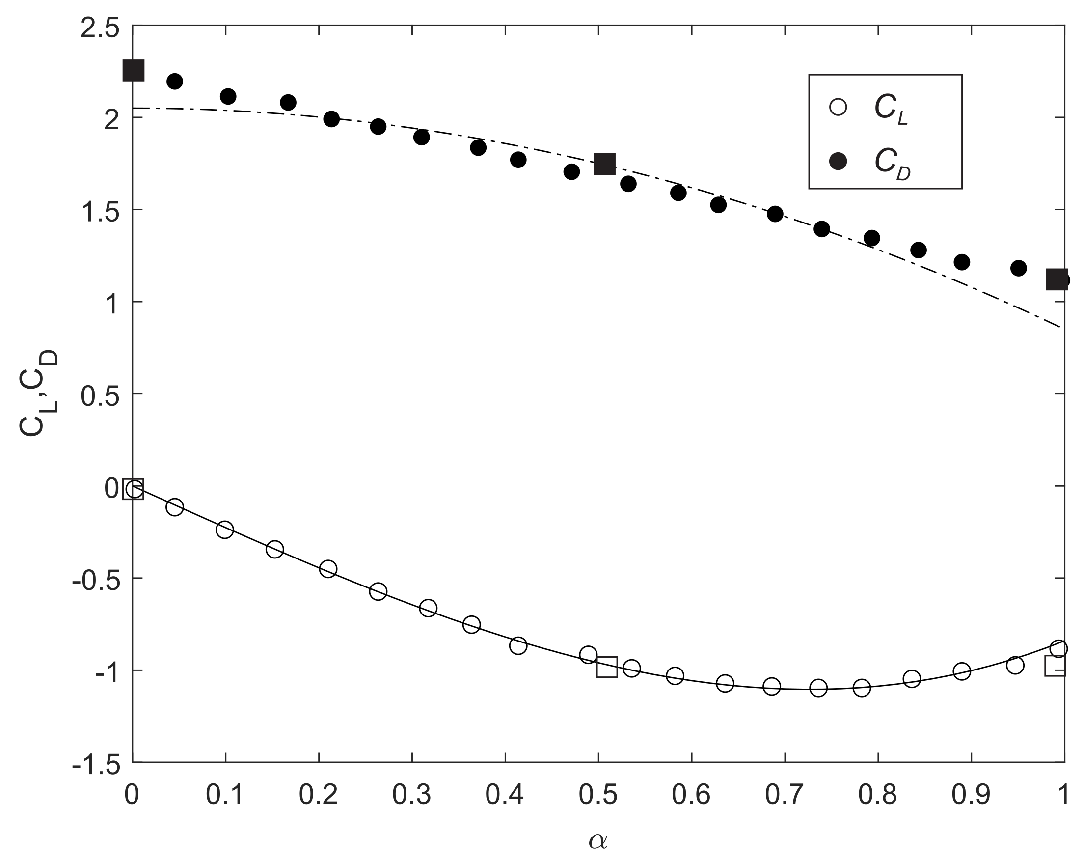
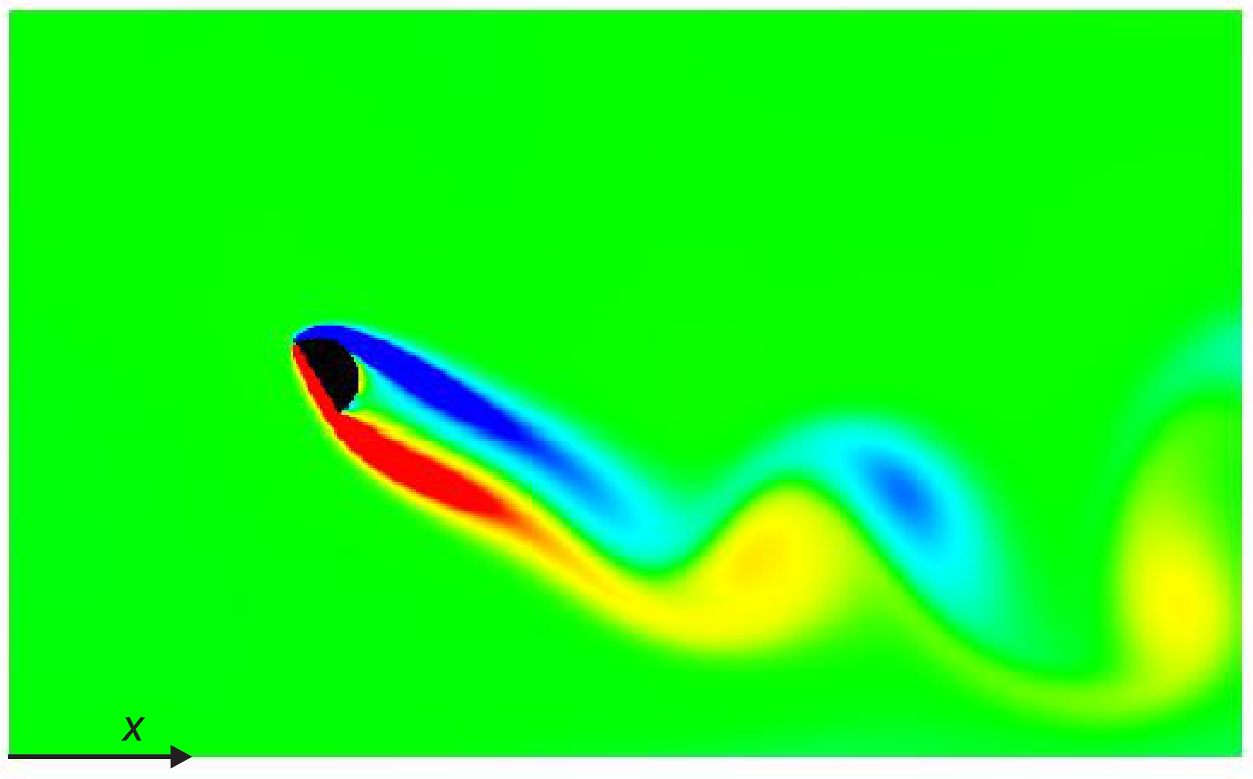
The computational domain and boundary conditions are shown in Figure 4. The diameter of the D-Section has 40 lattice points (observe that the number of lattice points for the diameter of the cylinder $N_D$ is linked to the Reynolds number $Re$, kinematic viscosity $\nu$, and inflow velocity U (free of turbulence), since $N_D=\nu Re/U$) and the computational domain chosen is 40D × 30D, giving a size of 1600 × 1200 lattice points. The left boundary was set to be a velocity specified inflow boundary condition with constant velocity profile U. To simulate the incompressible condition, the Mach number must be low enough; to this end, the inflow velocity U was set to 0.05 (the velocity of sound is $c_s=1/\sqrt{3}$ so that the Mach number at the inflow is $Ma=U\sqrt{3}$ and $M{a}^2$ is of order 0.01). The rest of the outer computational boundaries were considered outflows. For the boundary conditions on the body, a no-slip boundary condition has been applied that is fluid velocity equal to body velocity (see Appendix A for details about how physical boundary conditions are implemented).

3.2. Results

First of all, static numerical simulations were carried out to compute static drag and lift coefficients. To this end, no-motion was imposed ($Y=Y^{\prime }=Y^{\prime \prime }=0$) and a fixed angle of attack ($\theta$ fixed). Figure 5 shows the dependence of the lift and drag coefficients with the angle of attack $\alpha$ from the numerical simulations carried. As said before, the Reynolds number was 100. In addition, results from [20] are presented for validation purposes, as well as polynomial fitting curves obtained by least squares minimization (see Equation (5); $l_1=-2.28,l_3=1.44$, $d_0=2.05$ and $d_2=-1.20$).

In Figure 6left, the theoretical variation of galloping coefficients $\widetilde{a_1}$ and $\widetilde{a_3}$ with $K_1$ is shown. Note that this variation is obtained from Equations (11) and (12) once fitting coefficients for $C_L$ and $C_D$ are known. Figure 6right shows the transverse fluid force coefficient $C_Y$ as a function of the motion induced angle of attack ${\alpha }_M$, for different values of $K_1$ (see Equation (9)). It can be seen that, as $K_1$ is increased so is the maximum value of $C_Y$, but such maximum occurs for lower values of ${\alpha }_M$. In addition, increasing $K_1$ makes the curve of $C_Y$ with respect to ${\alpha }_M$ narrower and the cut of the curve with $C_Y=0$ occurs for lower values of ${\alpha }_M$, except for a small range between $0<K_1<0.3$.

Figure 7 presents steady-state amplitude of oscillations and energy harvesting efficiency as a function of the the reduced velocity for two different positive values of $K_1$. As can be seen, the quasi-steady theoretical model presented (Equation (16)) for the normalized amplitude of oscillations and Equation (22) for the efficiency) is capable of predicting fairly correctly the amplitude of oscillation and, to a lesser extent, the efficiency of energy harvesting when compared to the full fluid–structure–interaction numerical simulations which also showed a nearly sinusoidal response. For $K_1=0.5$, the maximum efficiency achieved is 0.14 (taken from numerical computations), whereas, for $K_1=1$, this figure has been increased to 0.16.

Figure 8 plots the maximum efficiency ${\eta }_{max}$ as a function of $K_1$ predicted by the theoretical model (Equation (24)) along with results obtained in numerical simulations. Agreement between theoretical model and computational results is good. Regarding computational results, for $K_1=0$, galloping solution without rotation, the maximum efficiency is ${\eta }_{max0}=0.05$. As $K_1$ is increased, the efficiency increases rapidly with $K_1$ until a maximum efficiency of ${\eta }_{max}=0.16$, obtained at $K_1=0.8$. Further increasing $K_1$ leads to a slow reduction of the maximum efficiency achievable. Therefore, through the rotation law investigated (and for a D-section at Reynolds 100), it is possible to increase the maximum achievable efficiency by a factor slightly higher than three times. It is noteworthy that the low efficiency for $K_1=0$ is mainly due to the Reynolds number (as it has a major effect on the detachment of the flow) and thus it is expected that, for the D-section at higher Reynolds number (or another cross-section shape), the maximum efficiency at $K_1=0$ will be higher and thus there will be a potential to obtain high values of ${\eta }_{max}$ thought the rotation actuation proposed.

It is interesting to study how much power is spent to rotate the body in order to see to what extent the hypothesis introduced in the theoretical model (that is, zero mean power to rotate the body) is valid. The mean power to rotate the body is:

$$P_R=\frac{1}{T}{\int }_0^T\left(M+\frac{1}{8}m{D}^2\ddot{\theta }\right)\dot{\theta }dt,$$

(29)

where T is an averaging time, M the fluid torque applied on the center of rotation, and $\dot{\theta }$ and $\ddot{\theta }$, respectively, the rotation velocity and acceleration.

Equation (29) can be made dimensionless dividing it by the kinetic power in the incoming flow:

$${\eta }_R=\frac{2P_R}{\rho U^{3}D}.$$

(30)

As an example, for a reduced velocity of $U^{*}=2.75$ and $K_1=0.5$, a value of ${\eta }_R=-0.0013$ was computed, whereas the efficiency of energy harvesting is 0.125, meaning that the power spent to rotate the body is around 1% of the power harvester. This result corroborates the idea taken from the quasi-steady analysis: the power spent to rotate the body should be small. Figure 9 shows numerical results obtained for $U^{*}=2.75$ and $K_1=0.5$, in terms of dimensionless amplitude of transverse oscillations (Figure 9a), fluid torque coefficient (Figure 9b), velocity of rotation and acceleration of rotations (Figure 9c). The following can be observed: (i) the transverse oscillations are quasi-sinusoidal, (ii) velocity and acceleration of rotating angle are nearly sinusoidal and there is almost a 90° phase shift between them so that the contribution to Equation (29) is nearly zero, and (iii) the torque is close to being in phase with rotation angle. These results explain that power spent to rotate the body is small.

For a better understanding from the physical point of view, the flow pattern (vorticity) around the galloping body is presented here for the case without actuation ($K_1=0$) and for a particular case with actuation ($K_1=1$), reduced velocity 4 and $\zeta =0.04$. In Figure 10, the wake structure after the body without actuation exhibits characteristic large-scale vortices being shed independently from the body’s oscillation at its own frequency. Thus, the wake pattern resembles that of a wave as each vortex is shed at different points of the cycle of oscillation following the Strouhal frequency of vortex emission for the body at rest ($f_v/f_N=St{U}^{*}$, where $St$ is the characteristic Strouhal number of the cross-section and $f_v$ the frequency of vortex shedding); thus, there is no synchronization between vortex shedding and oscillation.

On the other hand, in Figure 11, the wake after the body with actuation ($K_1=1$) exhibits a quite different flow pattern. Only independent vortices are formed at the point of maximum displacement during the cycle of oscillations when the body changes direction (maximum acceleration). The near-wake behind the body shows bounded vorticity which only breaks into an independent vortex downstream. This could be related to the fact that, through orientating the galloping body, it becomes much less bluff and the flow remains further attached.

For completeness, other cross-section shapes (equilateral triangle, rectangle and 45° rhombi) have been numerically simulated for $U^{*}=4$, $K_1=1$ (also $m*=10$ and $\zeta =0.04$). In terms of energy extraction efficiency, the following figures were obtained: $\eta =0.09$ for the D-shape, $\eta =0.04$ for the equilateral triangle, $\eta =0.01$ for the rectangular body (1:2 side relationship), and $\eta =0.001$ for the rhombus. From Figure 11 and Figure 12, it is seen that the most slender near-wake is given for the D-shape one.

4. Conclusions

The idea of imposing a rotation proportional to the motion-induced angle of attack on a galloping body has been studied, with its potential use for energy harvesting purposes in mind. A quasi-steady theoretical model to evaluate the dynamical behavior and the maximum efficiency of energy harvesting from Transverse Galloping with active pitch control has been developed and analyzed. The proposed model requires that the characteristic timescale of oscillation and rotation has to be much larger than the characteristic timescale of flow convection, which takes place usually under Transverse Galloping. In spite of the simplifications introduced in the model in order to arrive to analytical mathematical relationships (quasi-steady conditions, two term polynomial fitting of drag and lift coefficients, small motion-induced angle of attack, harmonic response), the present model is capable of correctly predicting the dynamics of oscillation as well as the energy harvested from the flow, with good agreement with computational results of the full fluid–solid interaction problem obtained through the Lattice Boltzmann Method. Note that the model may be useful as a design tool for practical implementations, for example to choose in advance the optimal rotating law (optimal $K_1$).

As a major result, it has been found that it is possible to increase importantly the efficiency of energy extraction (within the range of parameters tested), in particular, ${\eta }_{max}$ has been increased up to three times with respect to the case without active rotation. Thanks to the pitch control law chosen, proportional to the motion-induced angle of attack and hence linked to the body’s velocity, pitch variations are smooth and nearly sinusoidal (as the response of the body). To our knowledge, this type of active actuation linked to the body’s dynamics response and with energy harvesting purposes is suggested here for the first time, and can be of interest from both the basic and the applied side. In addition, it should be noted that the proposed active actuation could be of interest to diminish Transverse Galloping response, to protect a structural element—for example, fixing a negative value of $K_1$; as $K_1$ becomes more negative, $\widetilde{a_1}$ coefficient is diminished and galloping response is attenuated, in fact, for a high enough negative value of $K_1$, galloping is not possible. Finally, it should be noted that other rotating laws can be considered and should be evaluated.

References

1. Bernitsas, M.M.; Raghavan, K.; Ben-Simon, Y.; Garcia, E.M.H. VIVACE (Vortex Induced Vibration Aquatic Clean Energy): A New Concept in Generation of Clean and Renewable Energy from Fluid. J. Offshore Mech. Arct. Eng. ASME Trans. 2006, 130, 041101. [Google Scholar] [CrossRef]
2. Bernitsas, M.M.; Ben-Simon, Y.; Raghavan, K.; Garcia, E.M.H. The VIVACE Converter: Model Tests at Reynolds Numbers Around 105. J. Offshore Mech. Arct. Eng. ASME Trans. 2006, 131, 1–13. [Google Scholar]
3. Barrero-Gil, A.; Sanz-Andres, A.; Alonso, G. Energy Harvesting from Transverse Galloping. J. Sound Vib. 2006, 329, 2873–2883. [Google Scholar] [CrossRef] [Green Version]
4. Barrero-Gil, A.; Lopez, A.G.V.; Perez, J.R.A.; Acedo, Ó.P.; Ludlam, D.V.; Xu, J.X. Energy Converters and Energy Conversion Systems. U.S. Patent 9,541,058, 10 January 2017. [Google Scholar]
5. Sirohi, J.; Mahadik, R. Harvesting Wind Energy Using a Galloping Piezoelectric Beam. J. Vib. Acoust. 2010, 134, 011009. [Google Scholar] [CrossRef]
6. Sirohi, J.; Mahadik, R. Piezoelectric wind energy harvester for low-power sensors. J. Intell. Mater. Syst. Struct. 2011, 22, 2215–2228. [Google Scholar] [CrossRef]
7. Zhao, L.; Tang, L.; Yang, Y. Comparison of modeling methods and parametric study for a piezoelectric wind energy harvester. Smart Mater. Struct. 2013, 22, 125003. [Google Scholar] [CrossRef]
8. Yang, Y.; Zhao, L.; Tang, L. Comparative study of tip cross-sections for efficient galloping energy harvesting. Appl. Phys. Lett. 2013, 102, 064105. [Google Scholar] [CrossRef]
9. Xu-Xu, J.; Vicente-Ludlam, D.; Barrero-Gil, A. Theoretical study of the energy harvesting of a cantilever with attached prism under aeroelastic galloping. Eur. J. Mech. 2016, 60, 189–195. [Google Scholar] [CrossRef]
10. Blevins, R. Flow-Induced Vibrations, Van Nostrand Reinhold; Van Nostrand Reinhold Company: New York, NY, USA, 1990. [Google Scholar]
11. Naudascher, E.; Rockwell, D. Flow-Induced Vibrations: An Engineering Guide; A.A. Balkema: Rotterdam, Avereest, The Netherlands, 1994. [Google Scholar]
12. Païdoussis, M.P.; Price, S.J.; De Langre, E. Fluid-Structure Interactions: Cross-Flow-Induced Instabilities; Cambridge University Press: Cambridge, UK, 2011. [Google Scholar]
13. Abdelkefi, A.; Yan, Z.; Hajj, M.R. Performance analysis of galloping-based piezoaeroelastic energy harvesters with different cross-section geometries. J. Intell. Mater. Syst. Struct. 2014, 25, 246–256. [Google Scholar] [CrossRef]
14. Vicente-Ludlam, D.; Barrero-Gil, A.; Velazquez, A. Enhanced mechanical energy extraction from transverse galloping using a dual mass system. J. Sound Vib. 2015, 339, 290–303. [Google Scholar] [CrossRef] [Green Version]
15. Vicente-Ludlam, D.; Barrero-Gil, A.; Velazquez, A. Optimal electromagnetic energy extraction from transverse galloping. J. Fluids Struct. 2014, 51, 281–291. [Google Scholar] [CrossRef] [Green Version]
16. Abdelmoula, H.; Abdelkefi, A. Piezoaeroelastic investigation on the control and energy harvesting of galloping systems. In Proceedings of the 57th AIAA/ASCE/AHS/ASC Structures, Structural Dynamics, and Materials Conference, San Diego, CA, USA, 4–8 January 2016. [Google Scholar]
17. Rizzoni, G.; Hartley, T.T. Principles and Applications of Electrical Engineering; Mc-Graw Hill: New York, NY, USA, 2000. [Google Scholar]
18. Vicente-Ludlam, D.; Barrero-Gil, A.; Velazquez, A. Flow-induced vibration of a rotating circular cylinder using position and velocity feedback. J. Fluids Struct. 2017, 72, 127–151. [Google Scholar] [CrossRef]
19. Sorribes-Palmer, F.; Sanz-Andres, A. Optimization of energy extraction in transverse galloping. J. Fluids Struct. 2013, 43, 124–144. [Google Scholar] [CrossRef] [Green Version]
20. Bhinder, A.; Sarkar, S.; Dalal, A. Flow over and forced convection heat transfer around a semi-circular cylinder at incidence. Int. J. Heat Mass Transf. 2012, 55, 5171–5184. [Google Scholar] [CrossRef]
21. Higuera, F.J. Boltzmann approach to lattice gas simulations. EPL (Europhys. Lett.) 1989, 9, 663. [Google Scholar] [CrossRef]
22. Mei, R.; Luo, L.S.; Shy, W. An accurate curved boundary treatment in the lattice Boltzmann method. J. Comput. Phys. 1999, 155, 307–330. [Google Scholar] [CrossRef]
23. Zhou, Q.; He, X. On pressure and velocity boundary conditions for the lattice Boltzmann BGK model. Phys. Fluids 1997, 9, 1591–1598. [Google Scholar] [CrossRef] [Green Version]
24. Yu, D.; Mei, R.; Luo, L.S.; Shy, W. Viscous flow computations with the method of lattice Boltzmann equation. Progress Aerosp. Sci. 2003, 39, 329–367. [Google Scholar] [CrossRef]
25. Caiazzo, A.; Junk, M. Boundary forces in lattice Boltzmann: Analysis of momentum exchange algorithm. Comput. Math. Appl. 2008, 55, 1415–1423. [Google Scholar] [CrossRef]
Figure 1. Schematics of the forces acting on the galloping body.
Energies 13 00091 g001
Figure 2. Boundary of magnification factor equal to one, M = 1 , as a function of c 1 = d 0 / l 1 and c 2 = l 3 / d 2 .
Energies 13 00091 g002
Figure 3. Contour plot of maximum magnification factor M m a x as a function of c 1 = d 0 / l 1 and c 2 = l 3 / d 2 .
Energies 13 00091 g003
Figure 4. Schematics of the computational domain and boundary conditions. Detailed mesh around the cross-section is also shown.
Energies 13 00091 g004
Figure 5. C L and C D static coefficients dependence on the angle of attack (in radians) computed through numerical Lattice Boltzmann Method computations for a D-section at Re = 100. Polynomial fitting is shown with a solid line for C L ( l 1 = 2.28 , l 3 = 1.44 ) and dashed line C D ( d 0 = 2.05 and d 2 = 1.20 ) for For comparison purposes, results (squares) from [20] are also presented.
Energies 13 00091 g005
Figure 6. (left) Variation of a 1 ˜ and a 3 ˜ with K 1 . (right) Transverse fluid force coefficient C Y as a function of the motion induced angle of attack α M for different positive values of K 1 .
Energies 13 00091 g006
Figure 7. Normalized amplitude of oscillations A * and efficiency η as function of the reduced velocity U * for K 1 = 0.5 (a,b) and K 1 = 1 (c,d). White circles stand for results from the Lattice Boltzmann Method computations and solid lines from the quasi-steady model.
Energies 13 00091 g007
Figure 8. Maximum efficiency of energy harvesting as a function of K 1 . Results from Lattice Boltzmann Method computations are in white circles and theoretical predictions are from the quasi-steady model (Equation (24)).
Energies 13 00091 g008
Figure 9. (a) temporal evolution of the dimensionless transverse displacement of the body; (b) fluid torque coefficient evolution in time; (c) rotation speed and acceleration. U * = 2.75 , K 1 = 0.5 , m * = 10 , ζ = 0.04 , where a steady-state of oscillations has been reached.
Energies 13 00091 g009
Figure 10. Vorticity contour without actuation for a reduced velocity of U * = 4 , mass ratio m * is 10, and damping parameter ζ = 0.04 . The vorticity field when the body is at Y = 0 and going upwards is shown.
Energies 13 00091 g010
Figure 11. Vorticity contour with actuation ( K 1 = 1 ) for a reduced velocity of U * = 4 , mass ratio m * is 10, and damping parameter ζ = 0.04 . The vorticity field when the body is at Y = 0 and going downwards is shown.
Energies 13 00091 g011
Figure 12. Vorticity contour with actuation ( K 1 = 1 ) for a reduced velocity of U * = 4 , mass ratio m * is 10, and damping parameter ζ = 0.04 for equilateral triangle, rectangle (1:2 side), and 45° rhombi. It is shown the vorticity field when the body is at Y = 0 and going downwards.
Energies 13 00091 g012