A Systematic Approach to Predict the Economic and Environmental Effects of the Cost-Optimal Energy Renovation of a Historic Building District on the District Heating System

Abstract
:1. Introduction
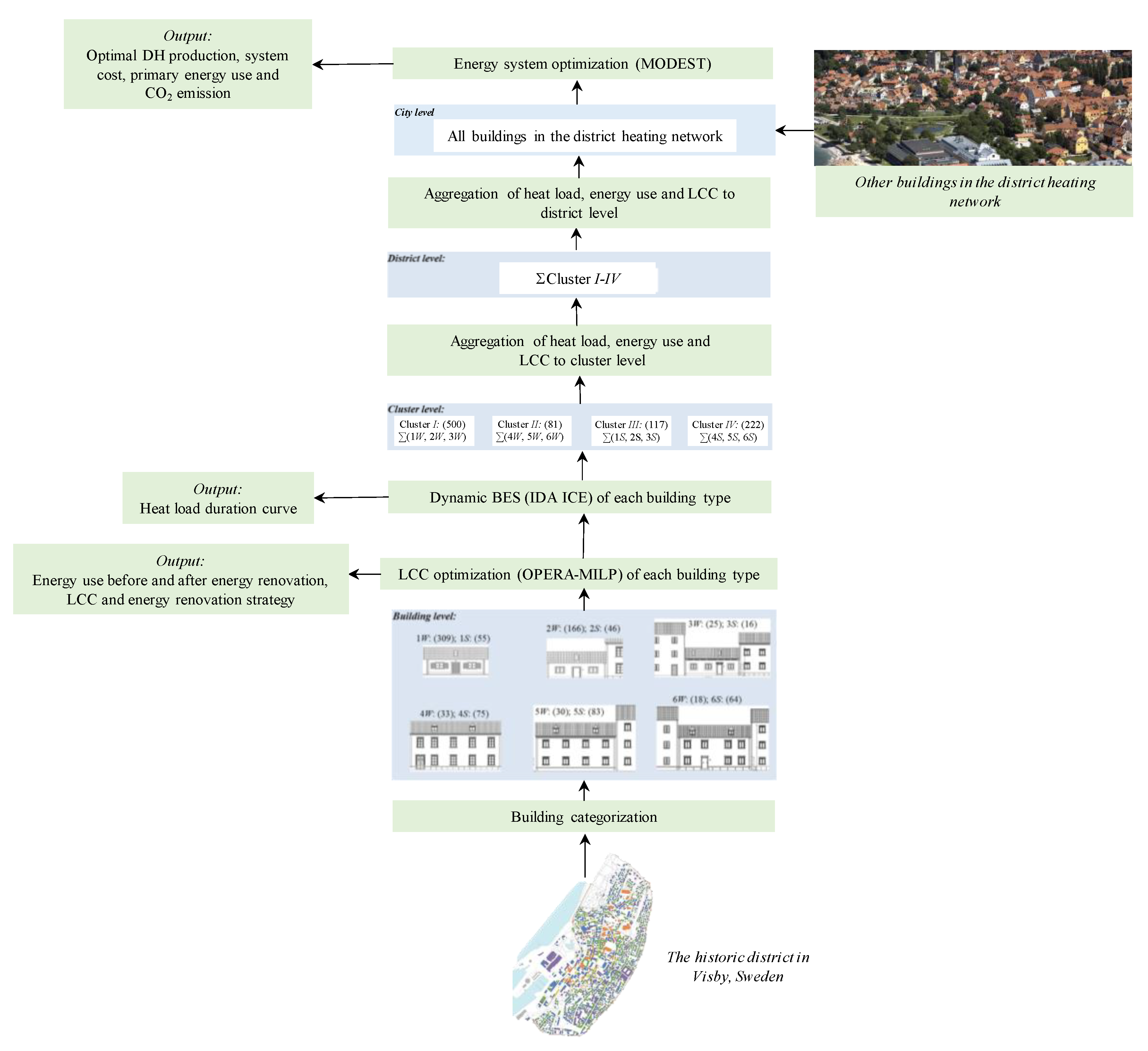
2. Systems Approach and Computational Tools
2.1. Life Cycle Cost Optimization in Buildings: OPERA-MILP
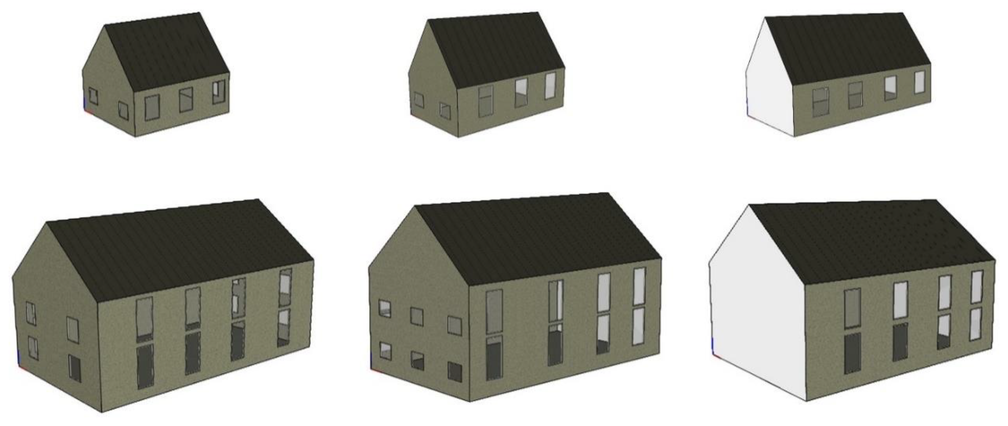
2.2. Building Energy Simulation: IDA ICE
2.3. Energy System Optimization: MODEST
3. Description of the Historic District and the District Heating System in Visby
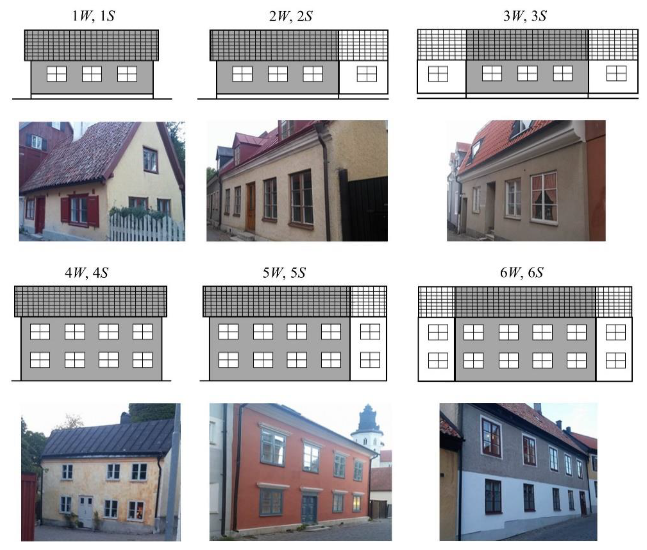
3.1. The Historic District
- Inventory of the building stock, i.e., gathering and compilation of building data;
- Categorization (allocating buildings in groups depending on the number of adjoining walls, number of stories and floor area);
- Selection of building types that are representative of the building stock (each building type selected based on average values of various building characteristics).
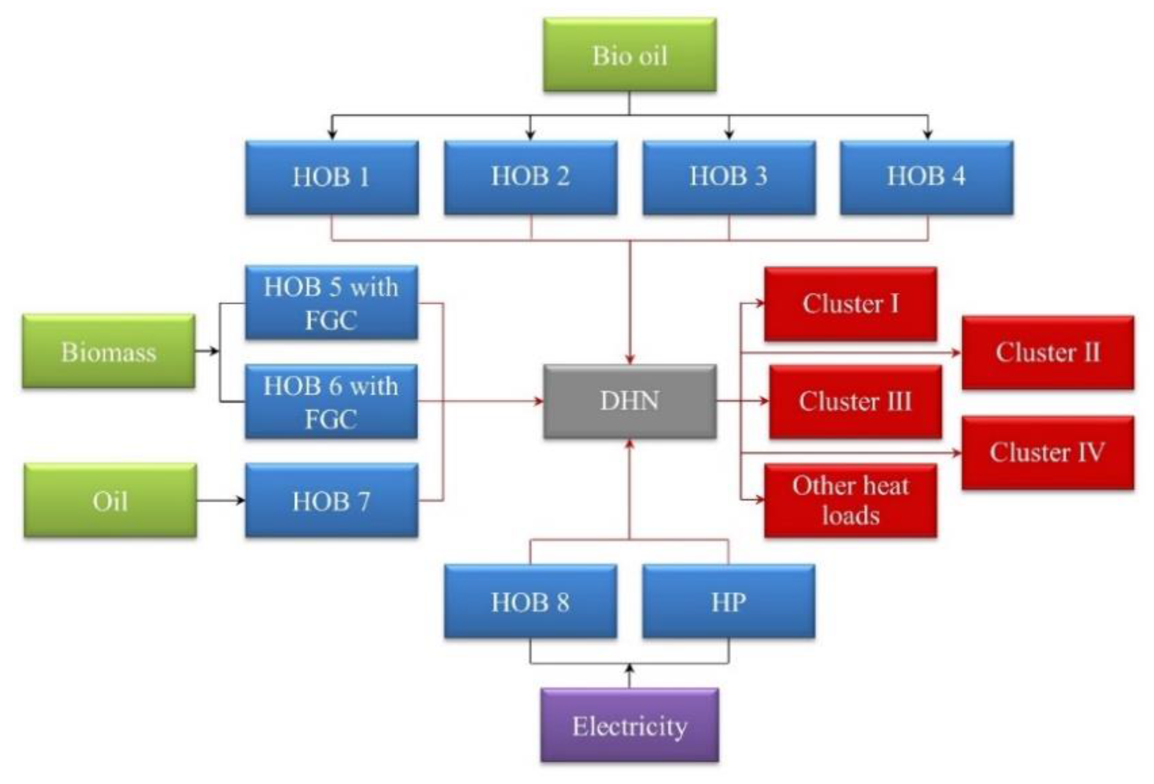
3.2. The District Heating System
4. Input Data
4.1. Input Data: OPERA-MILP
4.2. Input Data: IDA ICE
4.3. Input Data: MODEST
5. Results and Discussion
5.1. Energy Use, LCC, and System Cost, Net Income and Environmental Effects of the DH System before Energy Renovation of the Studied Buildings in Visby
5.1.1. Building Level
5.1.2. Cluster Level
5.1.3. District Level
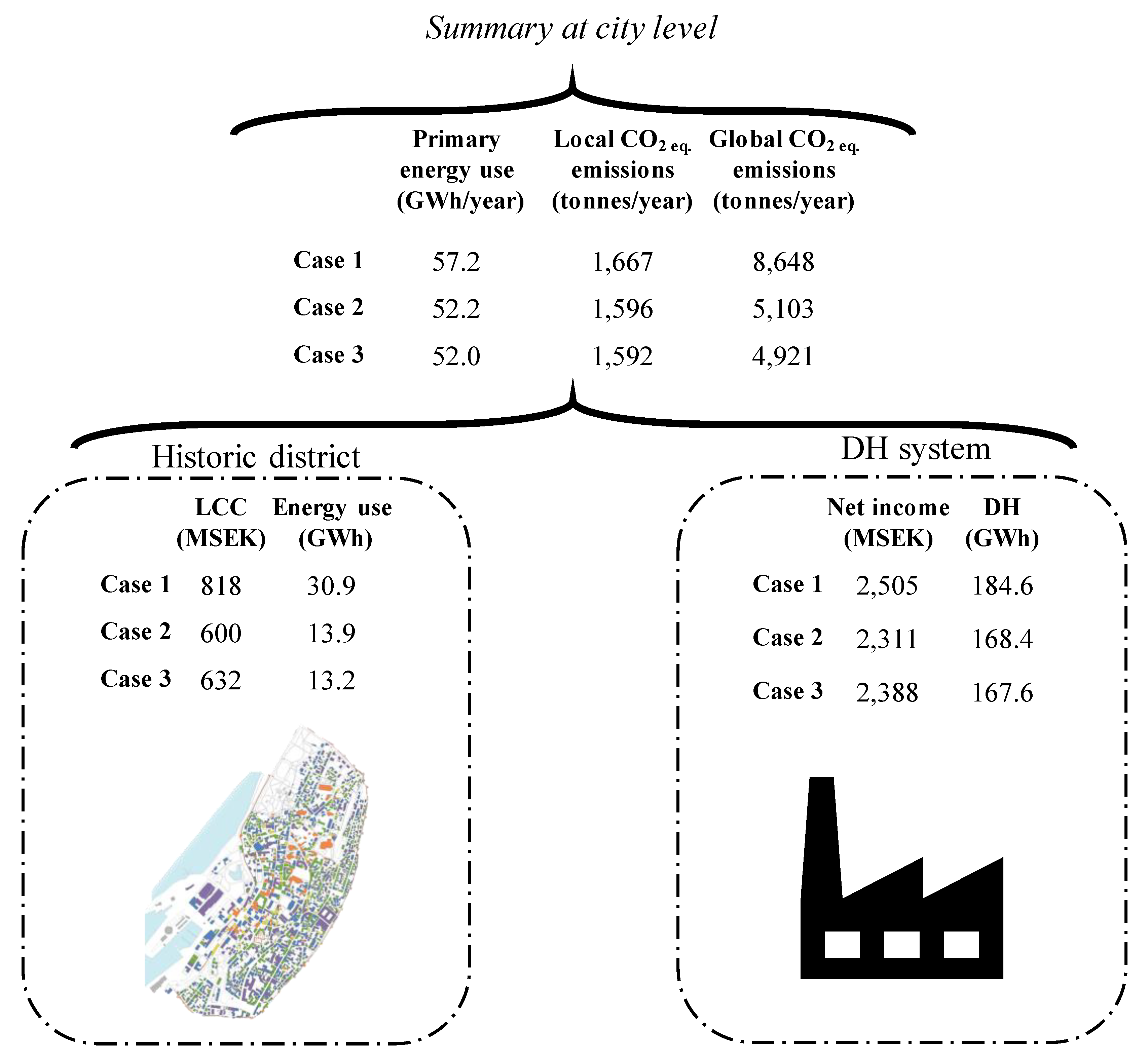
5.1.4. City Level
5.2. Cost-Optimal Energy Renovation; EEMs, Energy Use, LCC and System Cost, Net Income and Environmental Effects of the DH System
5.2.1. Building Level
- Floor insulation in the range between 24 cm and 32 cm is profitable for Cases 2 and 3 in Cluster I and Cluster III, i.e., building types standing on crawl space, because of high transmission losses originally
- Roof insulation is generally profitable in all clusters and cases because of low retrofit costs (despite an originally low U-value). The suggested insulation thickness varies between 10 and 18 cm at LCC optimum (Case 2). The corresponding figure for the energy target according to the Swedish building regulations (Case 3) for the building types varies more, due to the cost-effective comparison between EEMs on the building envelope
- Inside insulation of the external walls is profitable for all cases in the stone buildings, Cluster III and Cluster IV, because of a high U-value before renovation, 1.80–1.97 W/(m2·°C). The suggested insulation thickness is 20 cm in Case 2, but varies between 2 and 20 cm in Case 3, due to the cost-effective comparison between EEMs. The inside insulation of the external walls is also necessary in some of the wooden buildings to achieve the energy targets in Case 3.
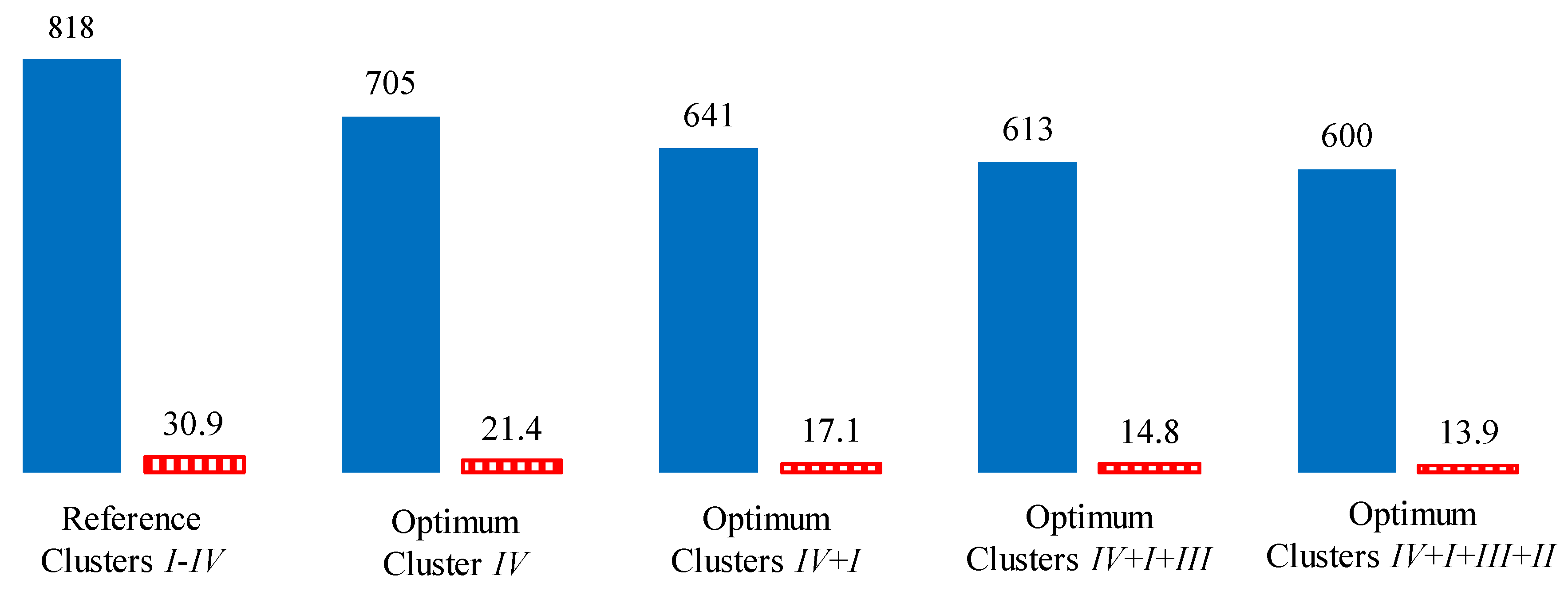
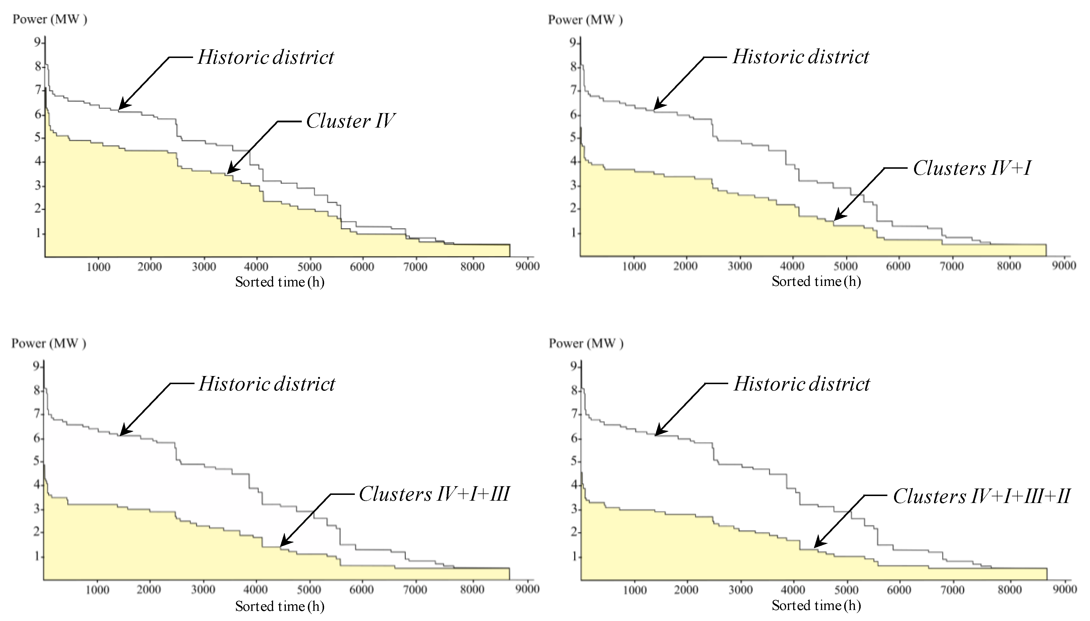
5.2.2. Cluster Level
5.2.3. District Level
5.2.4. City Level
6. Conclusions
Author Contributions
Funding
Acknowledgments
Conflicts of Interest
References
- U. Persson and S. Werner. Available online: http://www.heatroadmap.eu/resources/STRATEGO%20WP2%20-%20Background%20Report%204%20-%20Heat%20%26%20Cold%20Demands.pdf (accessed on 9 November 2017).
- The Swedish Energy Agency. Energy in Sweden 2019. An Overview; The Swedish Energy Agency: Stockholm, Sweden, 2019; ISSN 1404-3343. [Google Scholar]
- Artola, I.; Rademaekers, K.; Williams, R.; Yearwood, J. Boosting Building Renovation: What potential and value for Europe? 2016, PE 587.326; European Union: Brussels, Belgium, 2016. [Google Scholar]
- National Board of Housing, Building and Planning. Energy Use in Buildings-Technical Characteristics and Calculations-Results from the Project BETSI; National Board of Housing, Building and Planning: Karlskrona, Sweden, 2010; ISBN 978-91-86559-83-0.
- Liu, L.; Rohdin, P.; Moshfegh, B. Investigating cost-optimal refurbishment strategies for the medieval district of Visby in Sweden. Energy Build. 2017, 158, 750–760. [Google Scholar] [CrossRef]
- Åberg, M.; Henning, D. Optimisation of a Swedish district heating system with reduced heat demand due to energy efficiency measures in residential buildings. Energy Policy 2011, 39, 7839–7852. [Google Scholar] [CrossRef]
- Manfren, M.; Caputo, P.; Costa, G. Paradigm shift in urban energy systems through distributed generation: Methods and models. Appl. Energy 2011, 88, 1032–1048. [Google Scholar] [CrossRef]
- Åberg, M.; Widén, J. Development, validation and application of a fixed district heating model structure that requires small amounts of input data. Energy Convers. Manag. 2013, 75, 74–85. [Google Scholar] [CrossRef]
- Åberg, M. Investigating the impact of heat demand reductions on Swedish district heating production using a set of typical system models. Appl. Energy 2014, 118, 246–257. [Google Scholar] [CrossRef]
- Lundström, L.; Wallin, F. Heat demand profiles of energy conservation measures in buildingsand their impact on a district heating system. Appl. Energy 2016, 161, 290–299. [Google Scholar] [CrossRef] [Green Version]
- Le Truong, N.; Dodoo, A.; Gustavsson, L. Effects of heat and electricity saving measures in district-heated multistory residential buildings. Appl. Energy 2014, 118, 57–67. [Google Scholar] [CrossRef]
- Lidberg, T.; Gustafsson, M.; Myhren, J.A.; Olofsson, T.; Ödlund, L. Environmental impact of energy refurbishment of buildings within different district heating systems. Appl. Energy 2018, 227, 231–238. [Google Scholar] [CrossRef]
- Difs, K.; Bennstam, M.; Trygg, L.; Nordenstam, L. Energy conservation measures in buildings heated by district heating-A local energy system perspective. Energy 2010, 35, 3194–3203. [Google Scholar] [CrossRef] [Green Version]
- Lidberg, T.; Oloffson, T.; Trygg, L. System impact of energy efficient building refurbishment within a district heated region. Energy 2016, 106, 45–53. [Google Scholar] [CrossRef]
- Division of Energy Systems at Linköping University. Converter; Linköping University: Linköping, Sweden, 2016. [Google Scholar]
- Liu, L.; Rohdin, P.; Moshfegh, B. LCC assessments and environmental impacts on the energy renovation of a multi-family building from the 1890s. Energy Build. 2016, 133, 823–833. [Google Scholar] [CrossRef]
- Broström, T.; Eriksson, P.; Liu, L.; Rohdin, P.; Ståhl, F.; Moshfegh, B. A method to assess the potential for and consequences of energy retrofits in Swedish historic buildings. Hist. Environ. Policy Pract. 2014, 5, 150–166. [Google Scholar] [CrossRef]
- Gustafsson, S.-I. Mixed integer linear programming and building retrofits. Energy Build. 1998, 28, 191–196. [Google Scholar] [CrossRef]
- Gustafsson, S.-I. Optimal fenestration retrofits by use of MILP programming technique. Energy Build. 2001, 33, 843–851. [Google Scholar] [CrossRef]
- Henning, D. Optimisation of Local and National Energy Systems. Development and Use of the MODEST Model. Doctoral Dissertation, No. 559. Division of Energy Systems, Linköping University, Linköping, Sweden, 1999. [Google Scholar]
- Gebremedhin, A. A Regional and Industrial Co-Operation in District Heating Systems. Doctoral Dissertation, No. 849. Division of Energy Systems, Linköping University, Linköping, Sweden, 2003. [Google Scholar]
- Sundberg, G.; Henning, D. Investments in combined heat and power plants: Influence of fuel price on cost minimised operation. Energy Convers. Manag. 2002, 43, 639–650. [Google Scholar] [CrossRef]
- Sjödin, J.; Henning, D. Calculating the marginal costs of a district-heating utility. Appl. Energy 2004, 78, 1–18. [Google Scholar] [CrossRef]
- Henning, D.; Amiri, S.; Holmgren, K. Modelling and optimization of electricity, steam and district heating production for a local Swedish utility. Eur. J. Oper. Res. 2006, 175, 1224–1247. [Google Scholar] [CrossRef]
- Rolfsman, B. CO2 emission consequences of energy measures in buildings. Build. Environ. 2002, 37, 1421–1430. [Google Scholar] [CrossRef]
- Åberg, M.; Widén, J.; Henning, D. Sensitivity of district heating system operation to heat demand reductions and electricity price variations: A Swedish example. Energy 2012, 41, 525–540. [Google Scholar] [CrossRef]
- Weinberger, G.; Amiri, S.; Moshfegh, B. On the benefit of integration of a district heating system with industrial excess heat: An economic and environmental analysis. Appl. Energy 2017, 191, 454–468. [Google Scholar] [CrossRef]
- Amiri, S.; Henning, D.; Karlsson, B.G. Simulation and introduction of a CHP plant in a Swedish biogas system. Renew. Energy 2013, 49, 242–249. [Google Scholar] [CrossRef]
- Amiri, S.; Weinberger, G. Increased cogeneration of renewable electricity through energy cooperation in a Swedish district heating system-A case study. Renew. Energy 2018, 116, 866–877. [Google Scholar] [CrossRef]
- Berg, F. Categorising a Historic Building Stock—An Interdisciplinary Approach; UU-259149; Uppsala University: Uppsala, Sweden, 2015. [Google Scholar]
- Broström, T.; Donarelli, A.; Berg, F. For the categorisation of historic buildings to determine energy saving. Agathon Int. J. Archit. Art Des. 2017, 1, 135–142. [Google Scholar]
- Public Health Agency of Sweden. Common Advice about Indoor Tempeatures; FoHMFS 2014:17; Public Health Agency of Sweden: Stockholm, Sweden, 2014.
- Wikells. Section Facts 17/18-Techno-economic compilation.
- Adalberth, K.; Wahlström, Å. Energy Audit of Buildings-Apartment Buildings and Facilities; Swedish Standards Institute: Stockholm, Sweden, 2009; ISBN 978-91-7162-755-1. [Google Scholar]
- European Central Bank. Euro Exchange Rates. Available online: https://www.ecb.europa.eu/stats/exchange/eurofxref/html/eurofxref-graph-sek.en.html (accessed on 3 September 2018).
- Swedish Energy Agency and National Board of Housing, Building and Planning. Proposals for National Stragegy for Energy Efficiency Renovation of Building; Swedish Energy Agency and National Board of Housing, Building and Planning: Karlskrona, Sweden, 2013; ISBN 978-91-7563-049-6.
- Mälarenergi. Buy a New Heat Exchanger. Available online: https://www.malarenergi.se/fjarrvarme/for-husagare/kop-ny-fjarrvarmecentral (accessed on 27 November 2018).
- ASHRAE. ASHRAE IWEC2 Weather Files for International Locations. Available online: http://ashrae.whiteboxtechnologies.com/ (accessed on 2 March 2017).
- Swedenergy. Environmental Assessment of District Heating. Available online: https://www.energiforetagen.se/statistik/fjarrvarmestatistik/miljovardering-av-fjarrvarme/miljovarden-fran-tidigare-ar/ (accessed on 27 November 2018).
- Grönkvist, S.; Sjödin, J.; Westermark, M. Models for assessing net CO2 emissions applied on on district heating technologies. Int. J. Energy Res. 2003, 27, 601–613. [Google Scholar] [CrossRef]
- Swedenergy. Agreement in the Heating Market Committe 2018; Swedenergy: Stockholm, Sweden, 2018. [Google Scholar]
- The Swedish Energy Agency. Energy Statistics. Available online: http://www.energimyndigheten.se/statistik/den-officiella-statistiken/alla-statistikprodukter/ (accessed on 20 February 2019).
- Milić, V.; Ekelöw, K.; Moshfegh, B. On the performance of LCC optimization software OPERA-MILP by comparison with building energy simulation software IDA ICE. Build. Environ. 2018, 128, 305–319. [Google Scholar] [CrossRef]
- Vassileva, I.; Campillo, J.; Schwede, S. Technology assessment of the two most relevant aspects for improving urban energy efficiency identified in six mid-sized European cities from case studies in Sweden. Appl. Energy 2017, 194, 808–818. [Google Scholar] [CrossRef]
- Shen, P.; Braham, W.; Yi, Y. The feasibility and importance of considering climate change impacts in building retrofit analysis. Appl. Energy 2019, 233, 254–270. [Google Scholar] [CrossRef]
- Le Truong, N.; Gustafsson, L. Minimum-cost district heat production systems of different sizes under different environmental and social cost scenarios. Appl. Energy 2014, 136, 881–893. [Google Scholar] [CrossRef]


| Cluster | I | II | III | IV | |||||||||
|---|---|---|---|---|---|---|---|---|---|---|---|---|---|
| Building Type | 1W | 2W | 3W | 4W | 5W | 6W | 1S | 2S | 3S | 4S | 5S | 6S | |
| No. of Buildings | 309 | 166 | 25 | 33 | 30 | 18 | 55 | 46 | 16 | 75 | 83 | 64 | |
| Building structure | Wood | × | × | × | × | × | × | ||||||
| Stone | × | × | × | × | × | × | |||||||
| Basement type | Crawl space | × | × | × | × | × | × | ||||||
| Unheated basement | × | × | × | × | × | × | |||||||
| No. of adjoining walls | 0 | 1 | 2 | 0 | 1 | 2 | 0 | 1 | 2 | 0 | 1 | 2 | |
| External walls | Area (m2) | 86 | 61 | 45 | 245 | 180 | 116 | 80 | 57 | 43 | 235 | 173 | 112 |
| U-value (W/(m2·°C)) | 0.65 | 0.65 | 0.65 | 0.67 | 0.67 | 0.67 | 1.8 | 1.8 | 1.8 | 1.97 | 1.97 | 1.97 | |
| Windows | Area (m2) | 12 | 12 | 12 | 44 | 37 | 30 | 12 | 12 | 12 | 44 | 37 | 30 |
| U-value (W/(m2·°C)) | 2.9 | 2.9 | 2.9 | 2.9 | 2.9 | 2.9 | 2.9 | 2.9 | 2.9 | 2.9 | 2.9 | 2.9 | |
| Roof | Area (m2) | 71 | 79 | 92 | 170 | 159 | 159 | 65 | 73 | 86 | 161 | 150 | 150 |
| U-value (W/(m2·°C)) | 0.18 | 0.18 | 0.18 | 0.25 | 0.25 | 0.25 | 0.18 | 0.18 | 0.18 | 0.25 | 0.25 | 0.25 | |
| Floor | Area (m2) | 49 | 50 | 58 | 133 | 124 | 129 | 44 | 44 | 52 | 123 | 115 | 120 |
| U-value (W/(m2·°C)) | 1.10 | 1.10 | 1.10 | 0.23 | 0.23 | 0.23 | 1.10 | 1.10 | 1.10 | 0.23 | 0.23 | 0.23 | |
| Heated area (m2) | 98 | 100 | 116 | 398 | 372 | 387 | 87 | 88 | 104 | 369 | 345 | 360 | |
| Heated volume (m3) | 216 | 219 | 256 | 942 | 881 | 917 | 192 | 194 | 228 | 874 | 817 | 852 | |
| Air change rate (ACH) | 0.76 | 0.74 | 0.72 | 0.65 | 0.64 | 0.62 | 0.77 | 0.75 | 0.73 | 0.65 | 0.64 | 0.62 | |
| LCC/Energy Target | EEMs on the Building Envelope | Case No. |
|---|---|---|
| Reference | Not allowed | Case 1 |
| LCC optimum | Allowed | Case 2 |
| Swedish building regulations—83 kWh/m2 and 79 kWh/m2 for single-family houses and multi-family buildings, respectively | Allowed | Case 3 |
| EEMs | C1, SFH1/MFB2 (SEK/Window) | C2, DG3/TG4/TG+LE5 (SEK/m2 Window) | C3, wood/stone (SEK/m2) | C4, wood/stone (SEK/m2) | C5, wood/stone (SEK/m2·m) | C6 (SEK) | C7 (SEK/kW) | C8 (SEK/kW) |
|---|---|---|---|---|---|---|---|---|
| Weatherstripping | 441/617 | - | - | - | - | - | - | - |
| Window replacement | - | 6738/8492/12,169 | - | - | - | - | - | - |
| Roof insulation | - | - | 0/0 | 0/0 | 679/679 | - | - | - |
| Floor insulation | - | - | 0/0 | 242/242 | 799/799 | - | - | |
| External wall inside insulation | - | - | 153/153 | 908/1335 | 1267/1267 | - | - | - |
| External wall outside insulation | - | - | 407/407 | 2411/2571 | 1267/1267 | - | - | - |
| DH unit | - | - | - | - | - | 22,611 | 415 | 255 |
| Heating System Data | Fuel Price (SEK/MWh) | Annual Cost (SEK) | η (-) | Life Time (Years) |
|---|---|---|---|---|
| DH unit | 959 | 315 | 0.95 | 25 [37] |
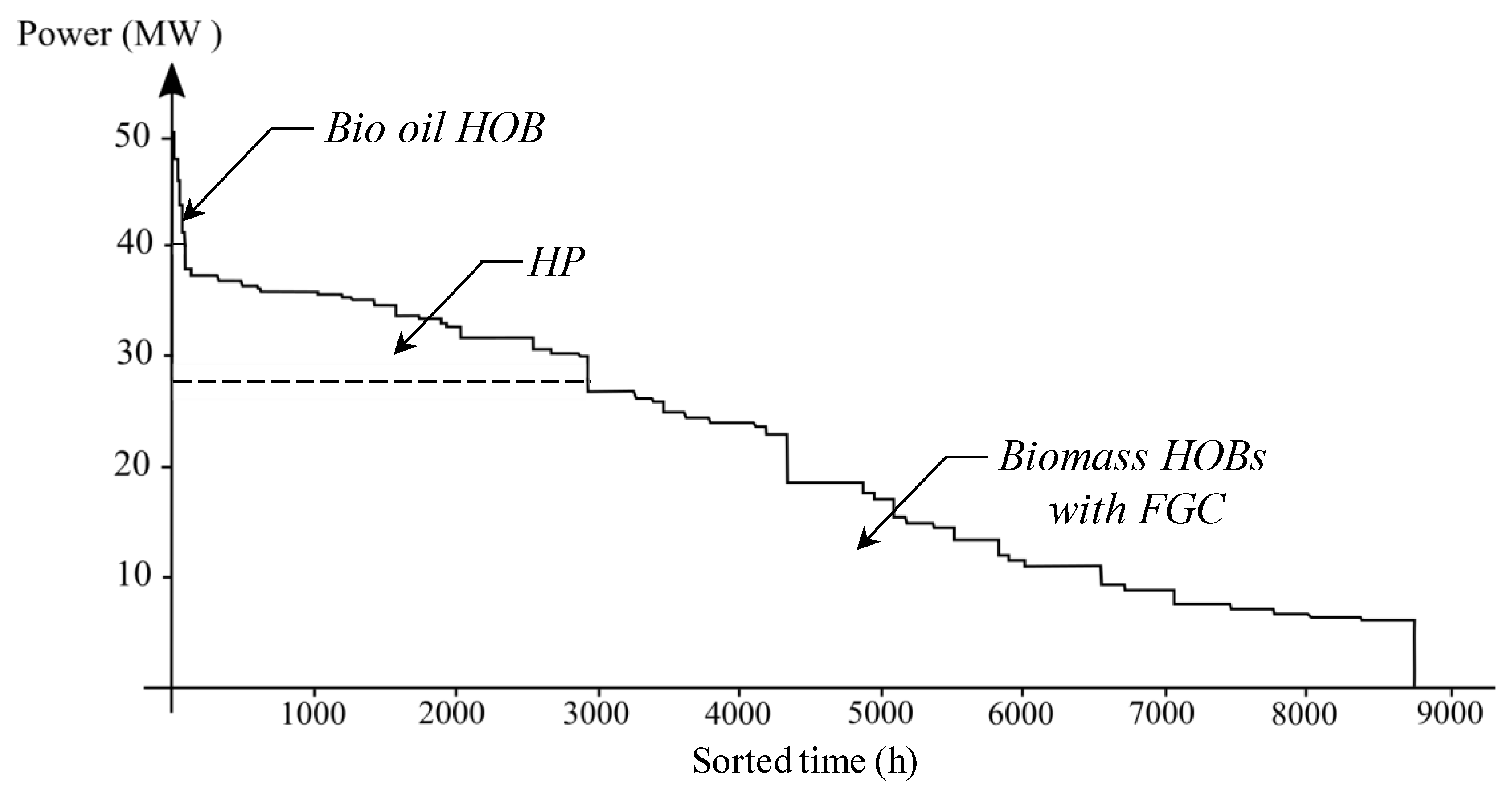
| Heat-Only Boilers/Heat Pump | Heat Production (MW) | Fuel | CO2 Emission Factor [40,41] (g CO2eq./kWh) |
|---|---|---|---|
| HOB 1 | 27.2 | Bio oil | 5 |
| HOB 2 | 10.8 | Bio oil | 5 |
| HOB 3 | 6 | Bio oil | 5 |
| HOB 4 | 11.8 | Bio oil | 5 |
| HOB 5 with FGC 1 | 10 | Biomass | 11 |
| HOB 6 with FGC 1 | 18 | Biomass | 11 |
| HOB 7 | 6.6 | Oil | 290 |
| HOB 8 2 | 17 | Electricity | 969 |
| Heat pump (HP) 3 | 12 | Electricity | 969 |
| Month | Days and Hours | Month | Days and Hours |
|---|---|---|---|
| November–March | Mon.–Fri., 6–7 | April–October | Mon.–Fri., 6–22 |
| Mon.–Fri., 7–8 | Mon.–Fri., 22–6 | ||
| Mon.–Fri., 8–16 | Sat., Sun. and holiday, 6–22 | ||
| Mon.–Fri., 16–22 | Sat., Sun. and holiday, 22–6 | ||
| Mon.–Fri., 22–6 | |||
| Sat., Sun. and holidays, 6–22 | |||
| Sat., Sun. and holidays, 22–6 | |||
| Top day, 6–7 | |||
| Top day, 7–8 | |||
| Top day, 8–16 | |||
| Top day, 16–22 | |||
| Top day, 22–6 |
| Cluster | I | II | III | IV | ||||||||
|---|---|---|---|---|---|---|---|---|---|---|---|---|
| Building Type | 1W | 2W | 3W | 4W | 5W | 6W | 1S | 2S | 3S | 4S | 5S | 6S |
| Maximum power demand (kW) | 6.9 | 6.4 | 6.7 | 19.0 | 16.3 | 14.4 | 9.1 | 7.8 | 7.6 | 27.3 | 22.2 | 17.9 |
| Specific energy use (kWh/m2) | 200.1 | 178.6 | 161.2 | 128.1 | 115.4 | 99.1 | 324.0 | 266.2 | 218.0 | 219.8 | 187.3 | 143.2 |
| Specific LCC (kSEK/m2) | 5.6 | 5.0 | 4.4 | 3.7 | 3.3 | 2.7 | 8.1 | 6.8 | 5.6 | 5.5 | 4.8 | 3.6 |
| Cluster | I | II | III | IV | ||||||||
|---|---|---|---|---|---|---|---|---|---|---|---|---|
| Building Type | 1W | 2W | 3W | 4W | 5W | 6W | 1S | 2S | 3S | 4S | 5S | 6S |
| No. of Buildings | 309 | 166 | 25 | 33 | 30 | 18 | 55 | 46 | 16 | 75 | 83 | 64 |
| Specific energy use (kWh/m2) | 200.1 | 178.6 | 161.2 | 128.1 | 115.4 | 99.1 | 324.0 | 266.2 | 218.0 | 219.8 | 187.3 | 143.2 |
| Specific energy use at the cluster level (kWh/m2) | 190.7 | 117.1 | 284.9 | 185.8 | ||||||||
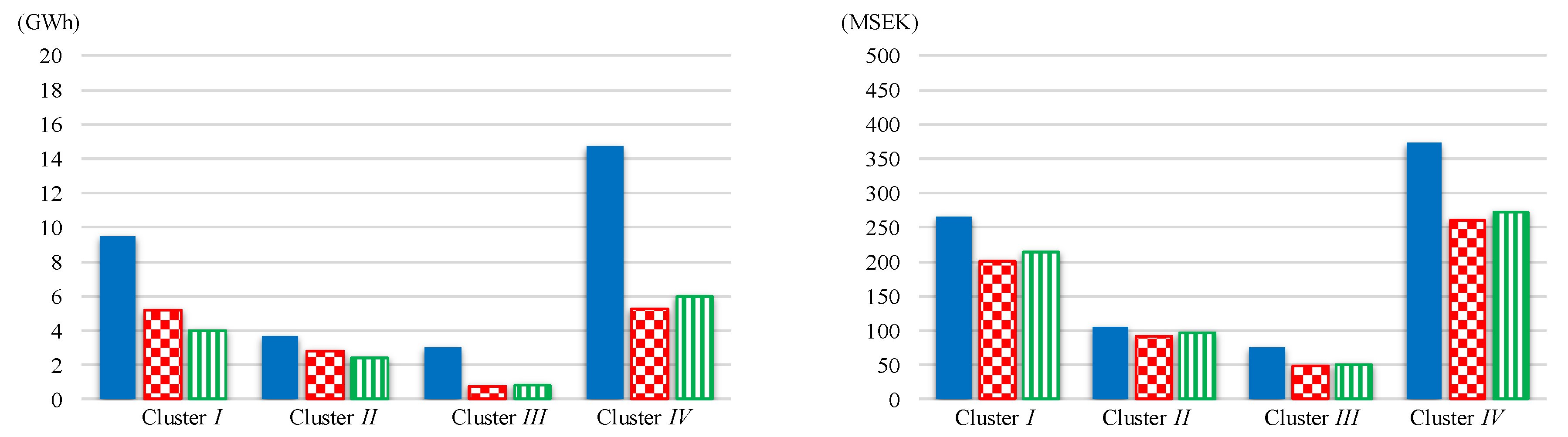
| Total energy use at the cluster level (GWh) | 9.5 | 3.7 | 3.0 | 14.7 | ||||||||
| Specific LCC (kSEK/m2) | 5.6 | 5.0 | 4.4 | 3.7 | 3.3 | 2.7 | 8.1 | 6.8 | 5.6 | 5.5 | 4.8 | 3.6 |
| Specific LCC at Cluster level (kSEK/m2) | 5.3 | 3.3 | 7.2 | 4.7 | ||||||||
| Total LCC at Cluster level (MSEK) | 263.8 | 103.2 | 75.6 | 372.9 | ||||||||
| Cluster | I | II | III | IV | |||||||||
|---|---|---|---|---|---|---|---|---|---|---|---|---|---|
| Building Type | 1W | 2W | 3W | 4W | 5W | 6W | 1S | 2S | 3S | 4S | 5S | 6S | |
| Window type | Case 2 | DG * | DG | DG | DG | DG | DG | DG | DG | DG | DG | DG | DG |
| Case 3 | DG | DG | DG | DG | DG | DG | DG | DG | DG | DG | DG | DG | |
| Floor insulation | Case 2 | 26 | 26 | 26 | 0 | 0 | 0 | 24 | 24 | 24 | 0 | 0 | 0 |
| Case 3 | 24 | 32 | 26 | 0 | 0 | 0 | 24 | 24 | 24 | 0 | 0 | 0 | |
| Roof insulation | Case 2 | 12 | 12 | 12 | 18 | 16 | 16 | 10 | 10 | 10 | 16 | 16 | 16 |
| Case 3 | 10 | 18 | 4 | 24 | 24 | 6 | 0 | 0 | 0 | 16 | 16 | 10 | |
| External wall inside insulation | Case 2 | 0 | 0 | 0 | 0 | 0 | 0 | 20 | 20 | 20 | 20 | 20 | 20 |
| Case 3 | 8 | 2 | 0 | 6 | 4 | 0 | 20 | 14 | 6 | 12 | 8 | 4 | |
| Cluster | I | II | III | IV | |||||||||
|---|---|---|---|---|---|---|---|---|---|---|---|---|---|
| Building Type | 1W | 2W | 3W | 4W | 5W | 6W | 1S | 2S | 3S | 4S | 5S | 6S | |
| Case 1 | kWh/m2 | 200.1 | 178.6 | 161.2 | 128.1 | 115.4 | 99.1 | 324.0 | 266.2 | 218.0 | 219.8 | 187.3 | 143.2 |
| kSEK/m2 | 5.6 | 5.0 | 4.4 | 3.7 | 3.3 | 2.7 | 8.1 | 6.8 | 5.6 | 5.5 | 4.8 | 3.6 | |
| Case 2 | kWh/m2 | 111.5 (−44) | 93.5 (−48) | 80.2 (−50) | 97.6 (−24) | 88.0 (−24) | 76.4 (−23) | 79.3 (−78) | 72.3 (−74) | 67.8 (−70) | 73.5 (−68) | 69.1 (−65) | 64.7 (−56) |
| kSEK/m2 | 4.3 (−24) | 3.7 (−26) | 3.1 (−28) | 3.2 (−14) | 2.9 (−14) | 2.4 (−14) | 5.6 (−37) | 4.7 (−35) | 3.8 (−34) | 4.0 (−32) | 3.5 (−30) | 2.7 (−27) | |
| Case 3 | kWh/m2 | 81.8 (−61) | 81.4 (−55) | 83.1 (−48) | 77.6 (−41) | 75.9 (−36) | 78.7 (−21) | 83.1 (−77) | 82.0 (−71) | 82.1 (−63) | 77.6 (−66) | 76.9 (−60) | 77.5 (−46) |
| kSEK/m2 | 4.7 (−20) | 4.1 (−18) | 3.2 (−28) | 3.5 (−8) | 3.2 (−7) | 2.4 (−13) | 5.7 (−36) | 4.8 (−34) | 3.9 (−32) | 4.0 (−31) | 3.5 (−28) | 2.9 (−21) | |
| Cluster | I | II | III | IV | ||||||||
|---|---|---|---|---|---|---|---|---|---|---|---|---|
| Building Type | 1W | 2W | 3W | 4W | 5W | 6W | 1S | 2S | 3S | 4S | 5S | 6S |
| No. of Buildings | 309 | 166 | 25 | 33 | 30 | 18 | 55 | 46 | 16 | 75 | 83 | 64 |
| Energy use before renovation—Case 1 (kWh/m2) | 190.7 | 117.1 | 284.9 | 185.8 | ||||||||
| LCC optimum—Case 2 (kWh/m2) | 103.7 (−46%) | 89.4 (−23%) | 74.7 (−76%) | 69.3 (−64%) | ||||||||
| Swedish building regulations—Case 3 (kWh/m2) | 81.7 (−57%) | 77.2 (−35%) | 82.5 (−73%) | 77.3 (−59%) | ||||||||
| LCC before renovation—Case 1 (kSEK/m2) | 5.3 | 3.3 | 7.2 | 4.7 | ||||||||
| LCC optimum—Case 2 (kSEK/m2) | 4.0 (−24%) | 2.9 (−12%) | 5.0 (−31%) | 3.4 (−28%) | ||||||||
| Swedish building regulations—Case 3 (kSEK/m2) | 4.4 (−17%) | 3.1 (−6%) | 5.1 (−29%) | 3.5 (−26%) | ||||||||
| Case | Energy Use (GWh) | LCC (MSEK) |
|---|---|---|
| Energy use before renovation—Case 1 | 30.9 | 818 |
| LCC optimum—Case 2 | 13.9 (−55%) | 600 (−27%) |
| Swedish building regulations—Case 3 | 13.2 (−57%) | 632 (−23%) |
| DH Production, CO2 Emissions, System Cost and Net Income | Case 1 | Case 2 | Case 3 |
|---|---|---|---|
| DH (GWh/year) | 184.6 | 168.4 | 167.6 |
| Energy supply (GWh/year) | |||
| Biomass | 149.7 | 143.4 | 143.0 |
| Electricity | 7.2 | 3.6 | 3.4 |
| Bio oil | 0.6 | 0.3 | 0.3 |
| System cost (MSEK/year) | 39.8 | 34.9 | 29.9 |
| System cost over 50 years (MSEK) | 726.7 | 637.3 | 546.0 |
| Net income DH system (MSEK) | 2505 | 2311 | 2388 |
| DH Production, CO2 Emissions, System Cost and Net Income | Case 1 | Cluster IV | Clusters IV + I | Clusters IV + I + III | Clusters IV + I + III + II |
|---|---|---|---|---|---|
| DH (GWh/year) | 184.6 | 175.7 | 171.4 | 169.3 | 168.4 |
| Energy supply (GWh/year) | |||||
| Biomass | 149.7 | 146.4 | 144.6 | 144 | 143.4 |
| Electricity | 7.2 | 5.1 | 4.2 | 3.8 | 3.6 |
| Bio oil | 0.6 | 0.5 | 0.4 | 0.4 | 0.33 |
| Local CO2 eq. emissions (ton/year) | 1667 | 1630 | 1610 | 1600 | 1596 |
| Global CO2 eq. emissions (ton/year) | 8648 | 6606 | 5718 | 5285 | 5203 |
| System cost (MSEK) | 726.7 | 675.5 | 653.6 | 640.8 | 637.3 |
| Net income DH system (MSEK) | 2505 | 2400 | 2347 | 2323 | 2311 |
© 2020 by the authors. Licensee MDPI, Basel, Switzerland. This article is an open access article distributed under the terms and conditions of the Creative Commons Attribution (CC BY) license (http://creativecommons.org/licenses/by/4.0/).
Share and Cite
Milić, V.; Amiri, S.; Moshfegh, B. A Systematic Approach to Predict the Economic and Environmental Effects of the Cost-Optimal Energy Renovation of a Historic Building District on the District Heating System. Energies 2020, 13, 276. https://doi.org/10.3390/en13010276
Milić V, Amiri S, Moshfegh B. A Systematic Approach to Predict the Economic and Environmental Effects of the Cost-Optimal Energy Renovation of a Historic Building District on the District Heating System. Energies. 2020; 13(1):276. https://doi.org/10.3390/en13010276
Chicago/Turabian StyleMilić, Vlatko, Shahnaz Amiri, and Bahram Moshfegh. 2020. "A Systematic Approach to Predict the Economic and Environmental Effects of the Cost-Optimal Energy Renovation of a Historic Building District on the District Heating System" Energies 13, no. 1: 276. https://doi.org/10.3390/en13010276