Acoustic Noise Computation of Electrical Motors Using the Boundary Element Method

Abstract

This paper presents a numerical method and computational results for acoustic noise of electromagnetic origin generated by an induction motor. The computation of noise incorporates three levels of numerical calculation steps, combining both the finite element method and boundary element method. The role of magnetic forces in the production of acoustic noise is established in the paper by showing the magneto-mechanical and vibro-acoustic pathway of energy. The conversion of electrical energy into acoustic energy in an electrical motor through electromagnetic, mechanical, or acoustic platforms is illustrated through numerical computations of magnetic forces, mechanical deformation, and acoustic noise. The magnetic forces were computed through 2D electromagnetic finite element simulation, and the deformation of the stator due to these forces was calculated using 3D structural finite element simulation. Finally, boundary element-based computation was employed to calculate the sound pressure and sound power level in decibels. The use of the boundary element method instead of the finite element method in acoustic computation reduces the computational cost because, unlike finite element analysis, the boundary element approach does not require heavy meshing to model the air surrounding the motor.

1. Introduction

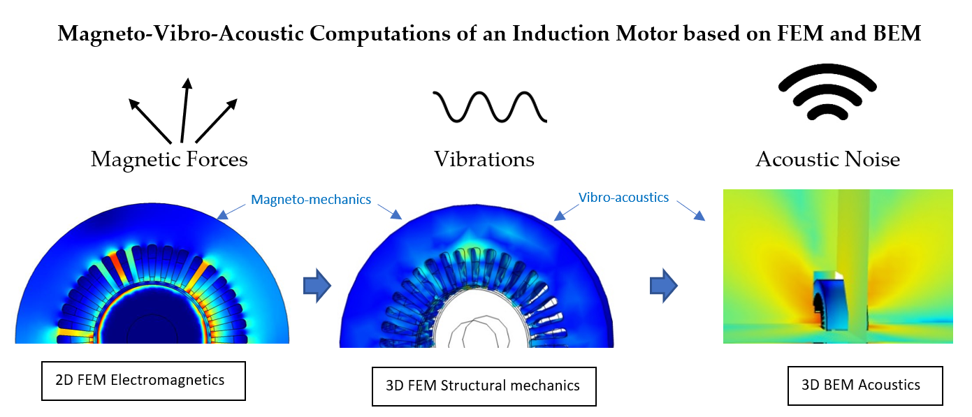
The acoustic noise in electric motors is a phenomenon of a complex nature and origin. The first kind, electromagnetic vibration and noise, is produced by magnetic forces, magnetostrictive expansion of the core laminations, eccentricity, phase unbalance, slot openings, and magnetic saturation. The second cause of noise is mechanical and is associated with mechanical assembly, in particular the bearings. The third major group is aerodynamic noise, which is due to the flow of ventilating air through or over the motor. These three sources are illustrated in Figure 1. A detailed review on the different forms of vibration and noise in electrical motors can be found in a paper by Vijayraghavan et al. [1]. One form of energy conversion happening in an electrical motor is from electrical energy to acoustic energy. The supply current interacts with the material to produce a magnetic field, which in turn produces magnetic forces. These forces excite the stator core and frame in the corresponding frequency range and produce mechanical vibrations. As a consequence of vibrations, the surface of the stator yoke and frame deforms with frequencies corresponding to the frequencies of forces. These stator and frame vibrations cause the surrounding medium of air to excite and vibrate and finally generate acoustic pressure variations (and thereby noise).

There have been various studies in the literature pertaining to the analysis of the vibrations and noise of electrical motors. Early stages of noise studies used analytical models and combined numerical and analytical methods. Belmans et al. carried out studies on the analytical formulation of acoustic noise in induction motors and authenticated the findings with experimental results [2]. They employed the rotating field theory with the Maxwell tensor method for calculating the frequency components produced by a motor that connect it to the airgap flux density time harmonics produced by the supply. The inference from their study was that high noise levels may be anticipated when one of the frequencies of the electromagnetically excited forces becomes the same as a natural frequency of the stator. They also developed a computerized model using finite element calculations and modal analysis that predicts the frequency components expected in the audible noise of a three-phase induction motor [3]. Cameron et al. have done measurement-based studies on vibrations and noise on reluctance motors and established that the stator deformation due to radial magnetic forces is the leading electromagnetic cause of noise [4]. Besnerais et al. demonstrated the impact of a Pulse Width Modulation (PWM) supply and switching frequencies on the magnetic noise of induction machines using analytical models [5]. Their approach was based on mechanical and acoustic 2D-ring stator models to compute the effect of winding space harmonics and PWM time harmonics in noise production [6]. Later on, Besnerais developed a multiphysical simulation tool for fast calculation of acoustic noise based on analytical and semi-analytical methods [7]. Their platform incorporated different models such as a permeance/magneto motive force (mmf) model, a subdomain model, and a finite element model. The semi-analytical models proved to be faster than the fully finite element models and had the same accuracy level, according to their evaluations. Devillers et al. studied the effect of tangential magnetic forces on vibrations and acoustic noise using a fast subdomain method to calculate Maxwell stress distribution and an electromagnetic vibration synthesis technique [8]. The same team later developed an experimental benchmark set-up for magnetic noise and a vibration analysis of electrical machines [9]. Fakam et al. coupled finite element structural analysis with an analytical tool to compute and compare the electromagnetic noise between surface permanent magnet and interior permanent magnet rotor topologies of a synchronous machine [10]. The same approach of a combined structural finite element method (FEM) and analytical methods was formulated by Islam et al. for computing sound power levels in synchronous motors [11].

With the improvement in numerical computational tools, the use of the boundary element method (BEM) or a combined FEM–BEM in noise computations became widespread. Moreover, these methods can give more accurate results in acoustic calculations. Juhl et al. developed a numerical method based on the BEM to calculate acoustic noise using the Helmholtz integral equation [12]. They created BEM-based numerical software for calculating sound fields on the exterior of bodies of three-dimensional shape or axisymmetric geometries [13]. Wang et al. used the BEM for computing sound power radiating from induction motors and a coupled structural FEM and acoustic BEM in their work [14]. Herrin et al. formulated a high-frequency BEM and compared it to the Rayleigh approximations method. They concluded that the high-frequency BEM is the more robust method [15]. Roivanen has employed different methods such as the BEM, high-frequency BEM, and plate approximation method combined with broad analytical, numerical, and experimental studies for calculating and comparing the sound power levels of electrical motors [16]. Neves et al. [17] presented a study on the coupling between magnetic forces, vibrations, and noise in a switched reluctance motor using FEM and BEM and gathered relatively good results. However, there were some mismatches between measured and simulated results that have been attributed to noise of aerodynamic origin. Furlan et al. [18] followed the same approach of a joint FEM–BEM-based analysis of a permanent magnet Direct Current (DC) electric motor. They simulated all three models, including an electromagnetic analysis in 3D, which could increase the memory requirements and computation time. In this paper, an electromagnetic simulation was done in 2D, and magnetic forces were taken from a 2D model and put into a 3D structural model. Schlensok et al. [19] presented an acoustic simulation of an induction machine with a squirrel-cage rotor, where 3D models were employed for electromagnetic, structural, and acoustic simulations. The electromagnetically excited structure- and air-borne noise of the motor was described in detail in their study. Deng et al. [20] investigated noise in an axial flux permanent magnet motor using electromagnetic and structural FEM and acoustic BEM; however, their approach also included a time-consuming complete 3D scheme. Järvenpää et al. [21] proposed a fast boundary element simulation of noise, where they imposed the surface velocity of a structural FEM model as a source of a fast BEM. This method facilitates the efficient modeling of large acoustic problems, although the computational cost is relatively high in this approach. Besides the computation of sound pressure in pascals and sound levels in dB surrounding the motor (shown in some previous studies), this paper also presents a far-field sound level calculation, which portrays the directivity of sound around the motor.

Inspired by the studies and findings in the literature, this paper investigated the aspect of vibro-acoustics in an electrical motor and formulated a practical and effective approach for acoustic noise calculation. The computational methodology and results successfully present a numerical technique for computing acoustic noise generated by an induction motor. The FEM- and BEM-based model describes how various quantities in different domains in an electrical motor can be calculated and used for acoustic analysis. An extensive numerical analysis of the magneto-mechanical and vibro-acoustic characteristics of a high-speed induction motor used for industrial applications is an original element of this study. Moreover, this paper paves a vivid path for researchers by detailing and clarifying the intricacies related to the preparation of a vibro-acoustic model of an electric motor by explaining both the theoretical and numerical implementation facets of the model. Although many studies have been carried out in this field of research, this paper brings an original contribution through a fully numerical analysis, the implementation of which is explained in detail.

2. Computational Methodology

This section explains our computational methods, including the main equations and numerical simulation stages employed for calculating the magnetic, mechanical, and acoustic quantities of the motor. Numerical modeling of noise generation in an electrical motor involves three models: first, modeling of the electromagnetic forces; then, modeling of the structural deformation and vibration behavior; and finally, modeling of the consequent acoustic response of the motor, as depicted in Figure 2.

2.1. Electromagnetics

The Maxwell equations of the magnetic field problem are solved numerically using 2D FEM. The Maxwell stress tensor method gives the magnetic torque exerted on a ferromagnetic region by integrating the magnetic stress over a surface around it [22]. Equation (1) is

$${\mathit{T}}_{em}=\underset{S}{\oint }\mathit{r}\times \mathit{\tau }\cdot dS=\underset{S}{\oint }\mathit{r}\times \left\{\frac{1}{{\mu }_0}(\mathit{B}\cdot \mathit{n})\mathit{B}-\frac{1}{2{\mu }_0}{\mathit{B}}^2\mathit{n}\right\}dS,$$

(1)

where $\mathit{\tau }$ is the Maxwell stress tensor, r is a vector representing the distance from the integration point to the torque axis, B is the magnetic flux density, ${\mu }_0$ is the permeability of the vacuum, and n is the normal unit vector of the integration surface dS. In an electrical machine, the integration surface is chosen as the outer surface of the rotor or any cylindrical surface in the airgap.

The magnetic force can be calculated from the Maxwell stress tensor by the volume integral ${\int }_V\nabla .\mathit{\tau }dV$. This volume integral can be reduced to the closed surface integral over a surface S, and the force formula becomes [23]

$$F=\underset{S}{\oint }\left\{\frac{1}{{\mu }_0}(\mathit{B}\cdot \mathit{n})\mathit{B}-\frac{1}{2{\mu }_0}{\mathit{B}}^2\mathit{n}\right\}dS=\underset{S}{\oint }\left(\frac{1}{2{\mu }_0}(B_n{}^2-B_t{}^2)\mathit{n}+\frac{1}{{\mu }_0}{B}_n{B}_t\mathit{t}\right)dS,$$

(2)

where t represents the outward unit vector tangential to the differential surface dS. The quantity inside the integral is usually interpreted as surface force density or traction. In this study, we follow the same interpretation and compute this force density on a surface located in the inner radius of the stator.

2.2. Structural Mechanics

Magnetic forces are the excitation parameters for the structural simulation of the stator core of the motor. The forces are fed to the stator elastic model as a body load in the simulation. The elastic model is represented by

$$\rho \frac{{\partial }^2\mathit{d}}{\partial t^2}-\nabla \cdot \tau =\mathit{f},$$

(3)

where $\rho$ is the mass density, d is the vector of displacements, and $f$ is the given volume force. After computing the displacements, a discrete Fourier transformation is performed using fast-Fourier transform (FFT), where the time-dependent solution is transformed from times to frequencies in the frequency domain.

2.3. Acoustics

The BEM used in this study is based on the direct collocation method [13], which deals directly with acoustic variables (sound pressure and particle velocity) and boundary conditions. The multiphysics coupling that combines FEM-and BEM-based physics is employed for coupling the results of solid mechanics finite element physics to acoustics boundary element physics. In the case of an electric motor, the vibrating stator boundary can be used as the acoustics FEM–BEM boundary to couple the acceleration from FEM computation to the BEM interface. This approach allows for modeling in an FEM–BEM framework using the strength of each formulation effectively. Acoustics physics solves the Helmholtz equation for constant-valued material properties and uses the pressure as the dependent variable. The wave equation can be solved in the frequency domain for one frequency at a time. The governing Helmholtz equation for a boundary element interface is given by

$$-\frac{1}{{\rho }_c}{\nabla }^2{p}_t-\frac{k_{cq}{}^2}{{\rho }_c}{p}_t=0,$$

(4)

$$k_{cq}{}^2={\left(\frac{\omega }{c_c}\right)}^2\mathrm{and} p_t=p+p_b$$

(5)

where $p_t$ is the total acoustic pressure, $K_{cq}$ is the wave number, ${\rho }_c$ is the density, $\omega$ is the angular frequency, and $c_c$ is the speed of sound in air.

The governing equations and boundary conditions are formulated using the total pressure $p_t$ with a scattered-field formulation. In the presence of a background pressure field defining a background pressure wave $p_b$, the total acoustic pressure $p_t$ is the sum of the pressure solved for p, which is then equal to the scattered pressure $p_s$ and the background pressure wave. The equations then contain information about both the scattered field and the background pressure field.

The benefit of the boundary element method is that only boundaries need to be meshed, and the degrees of freedom (DOFs) solved for are restricted to the boundaries. This is beneficial for handling complex geometries, as it introduces easiness in numerical computations. However, the BEM procedure results in fully populated or dense matrices, compared to the sparse system matrices in the FEM. Hence, the BEM is more expensive in terms of memory requirements per DOF than the FEM is, but it has fewer DOFs. Assembling and solving these can be very demanding. In this context, when solving acoustic models of small and medium size, the FEM will often be faster than solving the same problem with the BEM. This could be interpreted as one limitation of the BEM in small-sized computational models. However, in the case of the FEM, when the geometries are complex or two structures are far apart, large air domains need to be meshed. This is costly in terms of the numerical computational facet, as the frequency is increased.

The acoustic pressure computation problem involves solving for small acoustic pressure variations p in the surrounding medium of a sound source on top of the stationary background pressure $p_0$. In mathematical terms, this can be interpreted as a linearization of the dependent variables around the stationary quiescent values. The fluid flow problems in a compressible lossless fluid can be analyzed using the three governing equations, viz., the mass conservation equation or the continuity equation, the momentum conservation equation or Euler’s equation, and the energy equation or the entropy equation. They are given by

$$\frac{\partial \rho }{\partial t}+\nabla \cdot (\rho \mathit{u})=\mathit{M},$$

(6)

$$\frac{\partial \mathit{u}}{\partial t}+(\mathit{u}\cdot \nabla )\mathit{u}=-\frac{1}{\rho }\nabla p+\mathit{F},$$

(7)

$$\frac{\partial s}{\partial t}+\nabla \cdot (s\mathit{u})=0,$$

(8)

where $\rho$ is the total mass density, p is the total pressure, u is the velocity field, s is the entropy, and M and F are the possible source terms representing the body forces, if any. In conventional pressure acoustics scenarios, all thermodynamic processes are assumed to be isentropic in nature, which means the processes are both reversible and adiabatic. The small-parameter expansion is executed on a stationary fluid (u₀ = 0) of density ρ₀ (kg/m³) and at pressure p₀ (Pa) such that $p=p_0+p_1$ with $p_1\ll p_0$, $\rho ={\rho }_0+{\rho }_1$ with ${\rho }_1\ll {\rho }_0$, $\mathit{u}=0+{\mathit{u}}_1$ with ${\mathit{u}}_1\ll c$, and $s=s_0+s_1$.The small acoustic variations are represented by the variables with subscript 1. Inserting these values in the governing equations gives

$$\frac{\partial {\rho }_1}{\partial t}+\nabla \cdot ({\rho }_0{\mathit{u}}_1)=\mathit{M},$$

(9)

$$\frac{\partial {\mathit{u}}_1}{\partial t}=-\frac{1}{{\rho }_0}\nabla p_1+\mathit{F},$$

(10)

$$\frac{\partial p_1}{\partial t}=c_s{}^2(\frac{\partial {\rho }_1}{\partial t}+{\mathit{u}}_1\cdot \nabla {\rho }_0),$$

(11)

where $c_s$ is the isentropic speed of sound. The pressure time differential in the last equation is derived from the entropy equation. If the material parameters are constant, the last equation reduces to

$$p_1=c_s{}^2{\rho }_1.$$

(12)

This expression of acoustic pressure gives a condition that needs to be fulfilled for the linear acoustic equations to hold:

$$\left|p_1\right|\ll c_s{}^2{\rho }_0.$$

(13)

Finally, the transient wave equations for pressure waves in a lossless medium can be obtained by rearranging Equations (9)–(11) and dropping the subscripts:

$$\frac{1}{\rho c^2}\frac{{\partial }^{2}p}{\partial t^2}+\nabla \cdot [-\frac{1}{\rho }(\nabla p-q_d)]=Q_m,$$

(14)

where the source term $Q_m$ is a monopole domain source corresponding to a mass source and $q_d$ is a dipole domain source representing a domain force source. The speed of sound (c) and the density ($\rho$) may in general be space-dependent. The combination term $\rho c^2$ is called the adiabatic bulk modulus (K_s) with unit Pa, which is related to the adiabatic compressibility coefficient ${\beta }_s=1/K_s$.

In the frequency domain, the Helmholtz equation can be written as

$$\nabla \cdot [-\frac{1}{{\rho }_c}(\nabla p_t-q_d)]-\frac{k_{cq}{}^2{p}_t}{{\rho }_c}=Q_m.$$

(15)

Acoustics problems mostly encompass simple harmonic waves such as sinusoidal waves. In numerical computations, to model acoustic–structure interactions, a structural analysis can be coupled to acoustics by imposing the acceleration as a source in the boundaries of the structure in the form of normal acceleration, specified as

$$-\mathit{n}\cdot [-\frac{1}{{\rho }_c}(\nabla p_t-q_d)]=-\mathit{n}\cdot a_0,$$

(16)

where a₀ is the normal acceleration and q_d is the external force term.

2.4. Acoustic Pressure and Audible Sound

Sound is measured by changes in air pressure. The louder a sound is, the larger the change in air pressure is. The change here is the change from normal atmospheric pressure or reference pressure to the pressure disturbance caused by the sound. Sound pressure is measured in the unit “pascals”. A pascal (Pa) is equal to the force of one newton per square meter. The smallest sound pressure a human ear can hear is 20 µPa, which corresponds to zero dB. The sound pressure level (SPL) in dB can be calculated by

$$SPL = 20 lo{g}_{10}\left(\frac{p}{p_{ref}}\right) \mathrm{dB},$$

(17)

where $p_{ref}$ is the reference pressure 20 µPa in the case of audible sound calculations.

3. Results

The results of the numerical simulations are presented in this section. The simulations were done using COMSOL multiphysics software [24]. The specifications of the solid rotor induction motor are given in

Table 1. The solid rotor induction motor.

Specifications	Unit	Value
Power	kW	300
Voltage (line-to-line)	V	400
Rated speed	rpm	60,000
Number of poles		2
Stator outer diameter	mm	250
Stator inner diameter	mm	116

. The noise computation of an electric motor starts from the electromagnetic field computations, where the Maxwell equations are solved using finite element analysis. From the electromagnetic analysis, the forces of electromagnetic origin are taken into the mechanics domain to calculate the deformation and vibrations, where the forces are fed as an input to the solid mechanics calculations. Until the computation of vibrations, the FEM is used, and for the acoustic noise, the BEM is employed. In the first step, the electromagnetic simulation gives the magnetic forces due to Maxwell stress, and these forces are then fed to the structural computation as an input excitation. The supply frequency was 1008 Hz, and three time periods were simulated in the electromagnetic 2D computation. There were 19,750 linear triangular elements in the 2D mesh, as shown in Figure 3a, and the structural 3D mesh of the stator contained 104,931 tetrahedral elements, which is given in Figure 3b. 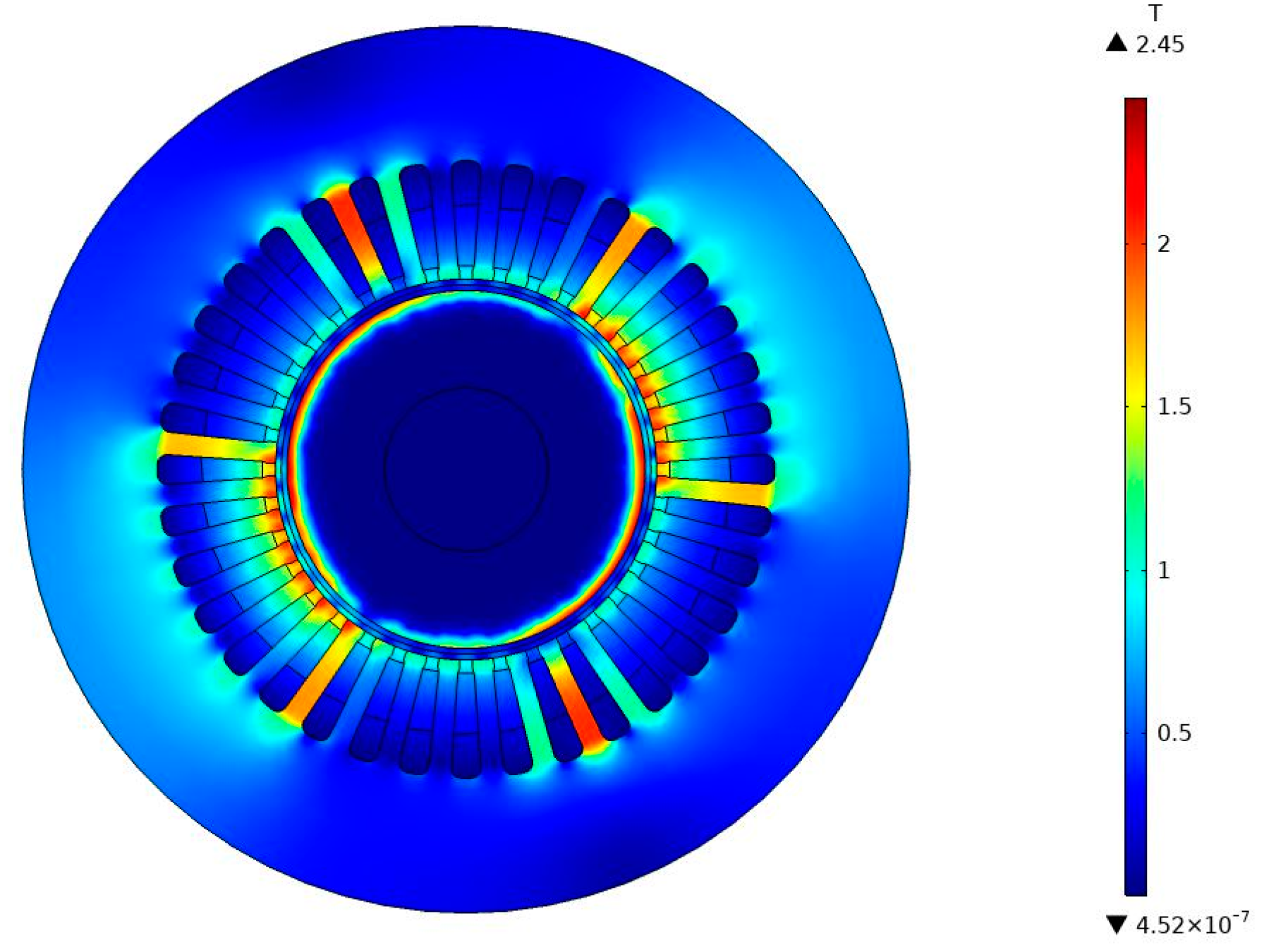Electromagnetic and structural mechanics time-stepping simulations were performed with a time-step length of 2.5 e⁻⁶ s for three time periods corresponding to a 0.003-s machine running time. The 2D electromagnetic computation took 17 min of CPU time to finish the simulation, and the 3D structural mechanics simulation took 4 h for each time period. A time-to-frequency FFT was done for the results of the third time period to transform the solution from a time to frequency domain. The acoustics computation to calculate the sound pressure level took 11 min of CPU time for each frequency. The magnetic flux density distribution across the cross-section of the motor is given in Figure 4.

In the structural simulation, displacement and acceleration of the stator body were computed. The magnetic forces were computed using Equation (2), and these forces were fed as the force term into Equation (3) to calculate the displacements. As a second stage of structural analysis, a Fourier analysis of the results was performed to discover the major frequency components in the deformation spectrum. The deformation pattern of the stator is depicted in Figure 5, and the Fourier analysis results of the displacement at a point on the stator outer surface are given in Figure 6, where the rotor rotational frequency is 1000 Hz, the twice-supply frequency, 2fs is 2016 Hz, and 4032 Hz corresponds to 2p*2fs, where p is the number of pole pairs.

In the final step of acoustics, the accelerations from the FE mechanics domain are imposed at the stator boundaries, as is theoretically explained in Equation (16). This specific feature couples acoustics with the structural analysis for an acoustic–structure interaction. For the acoustics computations, the air surrounding the motor is modeled as an infinite void, where no specific geometry or meshing is required. The BEM simulation calculates the acoustic pressure in the surrounding air of the motor and the resulting sound pressure level corresponding to different frequencies. Equation (15) is utilized in the calculation of sound pressure in the frequency domain. The acoustic pressure distribution outside the motor, corresponding to 2016 Hz of frequency, is shown in Figure 7. The sound pressure level produced by this acoustic pressure difference in the air is given in Figure 8. The same parameters for 4032 Hz are depicted in Figure 9a,b. Figure 10 shows the sound pressure level in far fields in different planes. The far-fields plots of the sound pressure level give a clear idea about the directivity of noise radiation in different planes around the motor at a particular frequency.

4. Discussion

The results presented in this paper showcase how magnetic forces produce acoustic sound in an electrical motor. The emphasis of this study was mainly centered on a sound level computation through FEM–BEM coupling, and the results show that this multilevel approach combining two numerical methods and three different physics in a single finite element tool is an effective tactic for acoustic analysis of electrical motors. The structural mechanics results provide information about the deformation and vibration behavior of the machine and also the major frequency components in the vibration spectrum, as is shown in Figure 5 and Figure 6. The computational results of the acoustic pressure variation occurring in the neighboring medium of the motor (Figure 7 and Figure 9a) shed light on the pattern of sound pressure and how different frequencies cause dissimilar forms of pressure variations in terms of their directions and intensity, thereby varying the levels of sound (Figure 8 and Figure 9b). The far-field sound pressure levels portrayed in Figure 10 offer an idea about how motor vibrations produce and direct sound in different directions.

One major drawback concerning numerical computations of acoustic noise is the relatively higher memory requirements and computational time required compared to analytical and semi-analytical models. The increased computational time of the FEM has been mentioned as a drawback of numerical methods in the literature, such as in References [7,8,9]. The use of the BEM in an acoustics domain fixes this issue to a considerable degree, without compromising the accuracy of the results. Although methods such as the permeance/mmf model [7,25] and the subdomain model [7,8,26] reduce the computational time, they possess some drawbacks in the modeling of complex geometries and in terms of the 3D effects of machines. In a multiphysical simulation environment, the use of the BEM instead of the FEM as the numerical method thus facilitates a competent framework for vibro-acoustic computations without compromising precision in detailed modeling, and it also has the benefit of reducing the computational time. If the FEM had been employed in the acoustic computations of the study presented in this paper, the entire surrounding air would have been meshed, and this would have caused increased memory requirements and computational time. A quantitative study comparing previous works could not be done because of the difference in motor types. However, qualitatively, the FEM–BEM approach has all of the benefits of numerical computations, especially in terms of accuracy and flexibility in modeling complex structures, and lessens the computational time significantly compared to a complete FEM model.

This paper does not include the measurement results of sound levels, and hence a future component of this study will be to conduct laboratory experiments to measure sound levels. In addition, to compare the measurement results to the simulations, the entire structure of the motor, including the frame and bearings, needs to be modeled in the future. Furthermore, computing and measuring the A-weighted sound levels corresponding to different frequencies need to be carried out in the second part of this study to precisely illustrate the sound pressure level in terms of human audibility [27]. In addition, in real-world problems where complex systems need to be simulated, materials cannot necessarily be connected: rather they are glued or clamped. Furthermore, the endplates and the frame of the motor could have an effect on the computed vibrations and sound pressures. Hence, the boundary layers in the structural FEM and acoustic BEM become more difficult to model. In those cases, accurate material models are required, and the model size could be increased. Both issues require measurements and iterative parameter adoption. However, the computational method presented in this paper facilitates a platform for vibro-acoustic studies by effectively modeling the acoustic noise of the motor.

5. Conclusions

The sound produced by an induction motor due to electromagnetic forces was successfully computed using a joint finite-element and boundary-element-based numerical computational technique. The energy conversion process in an electrical motor was modeled by showing how the electrical energy is converted into acoustic energy. The paper successfully illustrated how the proposed coupling methods and the FEM–BEM combination work effectively in acoustic studies of motors. The task of formulating a computational framework by combining theoretical equations in the right way and order, preparing numerical simulation stages, and coupling them to yield factual results in different stages and different physical domains was done in an original way in this study, as was presented in the paper. The proposed scheme is a vivid method describing how electromagnetic, mechanical, and acoustic domains can be analyzed and coupled in a numerical simulation platform. It provides an expedient and effectual tool for researchers in electrical machine and acoustics fields conducting magneto-mechanical and vibro-acoustics studies.