Modified Power Curves for Prediction of Power Output of Wind Farms

Abstract

Power curves are used to model power generation of wind turbines, which in turn is used for wind energy assessment and forecasting total wind farm power output of operating wind farms. Power curves are based on ideal uniform inflow conditions, however, as wind turbines are installed in regions of heterogeneous and complex terrain, the effect of non-ideal operating conditions resulting in variability of the inflow must be considered. We propose an approach to include turbulence, yaw error, air density, wind veer and shear in the prediction of turbine power by using high resolution wind measurements. In this study, two modified power curves using standard ten-minute wind speed and high resolution one-second data along with a derived power surface were tested and compared to the standard operating curve for a 2.5 MW horizontal axis wind turbine. Data from supervisory control and data acquisition (SCADA) system along with wind speed measurements from a nacelle-mounted sonic anemometer and wind speed measurements from a nearby meteorological tower are used in the models. The results show that all of the proposed models perform better than the standard power curve while the power surface results in the most accurate power prediction.

1. Introduction

As renewable energy becomes more prevalent, its integration into the power grid and the prediction of its energy contribution to the grid becomes more important. In the case of wind energy, prediction of power production is even more challenging due to its dependence on not only wind speed, but also meteorological conditions such as turbulence, wind shear, wind veer and air density. One way to predict power generation is by using wind forecasts as input for wind power models, which in turn predict wind power generation based on atmospheric boundary layer data. A model that accurately converts atmospheric data to wind power would be a powerful tool for power generation forecasting. The model that is typically used for this purpose is a standard power curve. Usually provided by wind turbine manufacturers, it relates ten-minute hub height wind speed to wind turbine power. However, evidence shows that only relating power output to hub height wind speed yields inaccuracy in power prediction. Clifton et al. [1] showed that power production can deviate by 5–10% compared to manufacturer’s power curve predictions and attributed the error to not accounting for turbulence. Additionally, the miss-alignment between the rotor and wind direction (yaw error) results in decreased power output and needs to be considered. Furthermore, there are a number of other atmospheric variables whose effect on power generation needs to be accounted for, including turbulence, density variation, wind shear and wind veer [2].

To improve wind power prediction, two approaches have been proposed:

(1)

A physics-based approach in which the effect of atmospheric variables are added to standard power curves. Wagner et al. [2,3] studied the effect of wind shear by proposing an equivalent wind speed using multiple measurements of wind speed distributed vertically. Additionally, methods to incorporate the effect of turbulence intensity [4,5,6,7] and yaw error [8] have been explored. The effect of atmospheric stability on the performance of power curves has also been examined [9,10]. Moreover, the applicability of equivalent wind speed extends beyond power curves. It can also be implemented in wind farm parameterization models such as Weather Research and Forecast (WRF) model [11].

(2)

A data-driven approach for modeling power production. Clifton et al. [1] used a machine learning algorithm called random forests (RF) to predict wind power and found that RFs are a very promising alternative to standard power curves. Neural networks [12,13], conditional kernel density [14] and support vector machines [15] are other data-driven models that have been investigated for power prediction.

In this work, we follow the physics-based approach for modeling power production. We expand on the existing power curve models and incorporate yaw error and turbulence using an equivalent wind speed, an approach which was introduced by Wagner et al. [3]. The equivalent wind speed combines the effect of turbulence and yaw error and represents them as a single variable at each height, which is then integrated vertically. Doing so forms a rotor equivalent wind speed to account for wind shear and wind veer. This rotor equivalent wind speed is used in a modified power curve the same way as hub height wind speed may be used in standard power curves.

2. Model Development

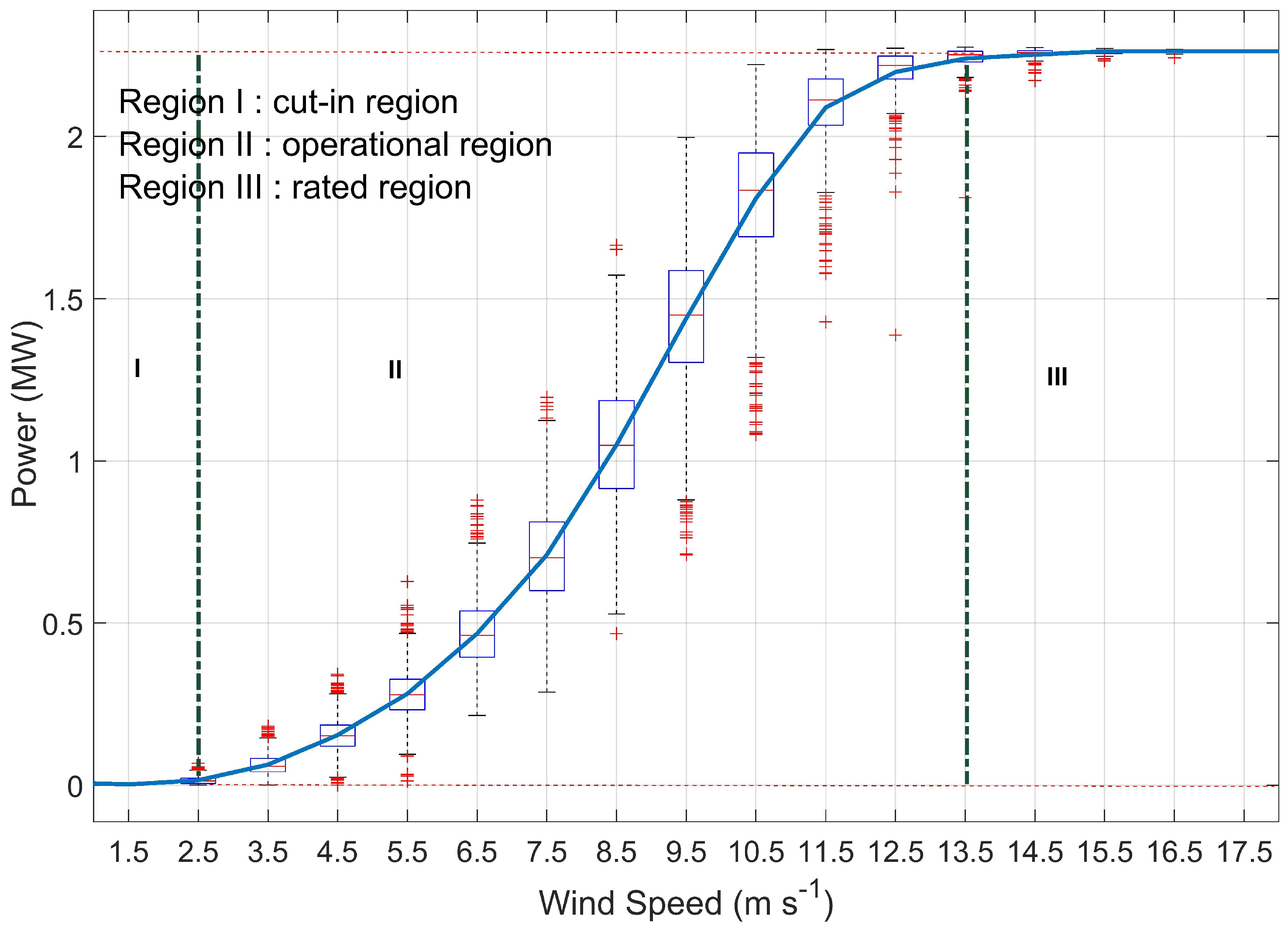
2.1. Standard Power Curve

Standard power curves provided by turbine manufacturers are based on a simple theoretical model following the IEC standard [16]. Theoretically, the amount of power generated by a wind turbine is modeled as a function of the area swept by the rotor blades, air density, and the kinetic energy flux into turbine rotor as:

$$P={\displaystyle \frac{1}{2}}\rho A{U}^3{C}_p,$$

(1)

where $\rho$ is air density, A is the rotor swept area, U is wind speed and $C_p$ is the power coefficient, which according to Betz’ calculations cannot exceed 0.593 [17]. Turbine designers optimize the design parameters for turbines such as the blade shape, rotor diameter and generator power based on annual wind forecast at an installation site and provide the power curve for the designed turbine [1]. In the case of the 2.5 MW wind turbine studied in this work, the manufacturers considered different constant values for air density for the provided power curves.

Wind turbine power performance measurements are based on Equation (1). To estimate the turbine power curve, wind speed and power output of the turbine are measured simultaneously. These measurements are then averaged over ten minute intervals to produce the power curve (power vs. wind speed) and power coefficient curve ($C_p$ vs. wind speed). For generating power curves, measurement of wind speed from a meteorological tower and power from SCADA is needed. Wind speed can also be measured using nacelle-mounted anemometers. Recently, nacelle mounted LIDARs have been used as an alternative to anemometers [18,19]. However, wind speeds measured at the nacelle do not accurately represent the inflow due to the effect of the rotor on the flow. Therefore, a nacelle transfer function (NTF) can be used for correcting wind speed measurements at the nacelle [20], which itself is only valid under strict criteria. Once the power curve is generated, it can be used to predict power generation from the wind turbine. Wind turbine power curves, as shown in Figure 1, consist of three main regions: cut-in region (I); operational region (II); and rated region (III). More information about power curves and how they are generated can be found in [16,17,20].

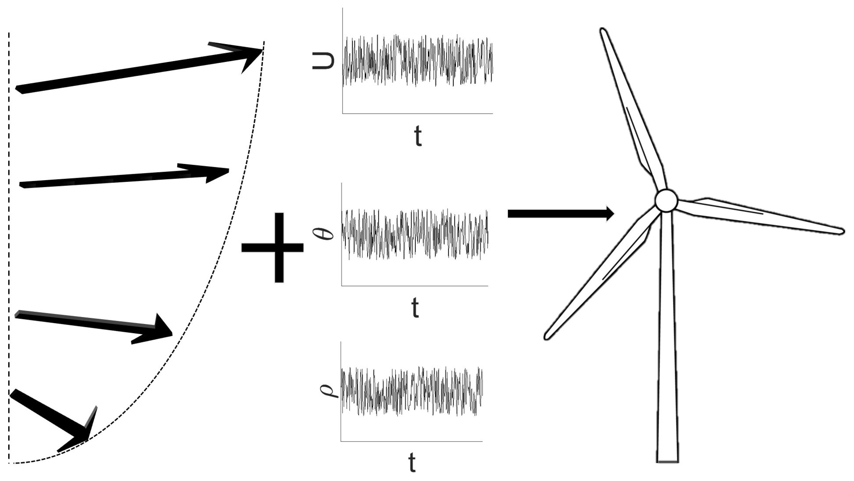
2.2. Modified Power Curves

We developed two variations of modified power curves: a model based on one-second data and a model based on ten-minute data. These modified power curves are based on equivalent wind speeds, generated through combining the effect of turbulence and yaw error. Moreover, a power surface was introduced in the end, which follows a two-dimensional binning and outperforms the other two models. Figure 2 shows the different variables implemented in these models.

2.2.1. Modified Power Curve Based on One-Second Data

The proposed one-second power curve includes yaw error, turbulence, and air density in addition to hub height wind speed in order to increase the accuracy of the model. In this version of the model, atmospheric data at a rate of 1 Hz are used.

Equation (1) relates how air density affects power production, and to address that, the power curve provided by the manufacturer considers variable air densities. Air density can vary over time, even over the course of diurnal cycles. Thus, the standard power curve needs to be adjusted for these variations, recommended by IEC [16] normalizing measured air density ($\rho \left(t\right)$) with respect to a reference value (${\rho }_0$). Following this approach, wind speed and air density are combined into a single variable while the unit of wind speed is conserved. Based on the IEC standard, the reference value for air density is taken to be air density at sea level (1.225 kg·m⁻³). The adjustment for density variation can be implemented as follows [16]:

$$U_{\rho }(t,z)=U(t,z){({\displaystyle \frac{\rho (t,z)}{{\rho }_0}})}^{1/3},$$

(2)

where $U_{\rho }$ is wind speed adjusted for density variations, U is the measured value of wind speed, $\rho$ is measured air density and ${\rho }_0$ is the reference air density.

A wind turbine cannot align with the inflow at all times because of the inherent variability of inflow wind direction. Therefore, only the normal component of the inflow, which is the component of wind that contributes to power production, should be included in the model. The normal component of the density adjusted wind speed is:

$$U_{\rho n}(t,z)=U_{\rho }(t,z)cos\left(\theta (t,z)\right),$$

(3)

where $\theta (t,z)$ is the angle between the wind speed and rotor as a function of time and height. Hence, the amount of power extracted by the turbine as a function of heights is:

$$P(t,z)={\displaystyle \frac{1}{2}}{\rho }_0{C}_p{A}_i{U}_{\rho n}{(t,z)}^3,$$

(4)

where $P(t,z)$ is the generated power as a function of time and height, $A_i$ is a sub-region of the rotor swept area, and $C_p$ is the power coefficient. From this point forward, $U_{\rho n}$$(t,z)$ is denoted as $U_{\rho n}$ for conciseness.

To account for turbulence, Reynolds decomposition is performed on $U_{\rho n}$:

$$U_{\rho n}=\overline{U_{\rho n}}+{U_{\rho n}}^{\prime },$$

(5)

where $\overline{U_{\rho n}}$ is the mean and ${U_{\rho n}}^{\prime }$ is the fluctuating part of velocity. Substituting Equation (5) into Equation (4), we get:

$$P(t,z)={\displaystyle \frac{1}{2}}{\rho }_0{C}_p{A}_i{(\overline{U_{\rho n}}+{U_{\rho n}}^{\prime })}^3={\displaystyle \frac{1}{2}}{\rho }_0{C}_p{A}_i({\overline{U_{\rho n}}}^3+3{\overline{U_{\rho n}}}^2{U_{\rho n}}^{\prime }+3\overline{U_{\rho n}}{U_{\rho n}}^{{\prime }^2}+{U_{\rho n}}^{{\prime }^3}).$$

(6)

Applying Reynolds averaging for P and neglecting the term $\overline{{U_{\rho n}}^{{\prime }^3}}$ results in an equation for time averaged power:

$$\overline{P}\left(z\right)={\displaystyle \frac{1}{2}}{\rho }_0{C}_{p}A({\overline{U_{\rho n}}}^3+3\overline{U_{\rho n}}\overline{{U_{\rho n}}^{{\prime }^2}}).$$

(7)

Denoting $\overline{{U_{\rho n}}^{{\prime }^2}}$ as ${\sigma }_{U_{\rho n}}^2$, the equivalent wind speed is:

$${U_{eq\rho }}_s\left(z\right)=\sqrt[3]{{\overline{U_{\rho n}}}^3+3\overline{U_{\rho n}}{\sigma }_{U_{\rho n}}^2}.$$

(8)

Subsequently, ${U_{eq\rho }}_s$ is integrated vertically over the rotor swept area, resulting in a rotor equivalent wind speed, as proposed by Wagner et al. [3]:

$${U_{req\rho }}_s={\displaystyle \frac{1}{A}}\sum _i{A}_i{U_{eq\rho }}_{i}i=1,2,\dots ,n,$$

(9)

where n is the number of heights at which wind speed is measured and i denotes each specific height. The time average power is then:

$$\overline{P}={\displaystyle \frac{1}{2}}{\rho }_0{C}_{p}A{{U_{req\rho }}_s}^3,$$

(10)

where ${U_{req\rho }}_s$ is the rotor equivalent wind speed and $A_i$ is the portion of the rotor area corresponding to the height where the wind speed measurement is taken. Subscript s in ${U_{eq\rho }}_s$ and ${U_{req\rho }}_s$ denotes that equivalent wind speeds and rotor equivalent wind speed are generated using one-second data. This rotor equivalent wind speed is then used to generate a modified power curve, in the same manner as standard power curves. It should be noted that, in Equation (10), both $\overline{P}$ and ${U_{req\rho }}_s$ are averaged over ten-minute periods, and wind turbine power is not predicted at 1 Hz.

2.2.2. Modified Power Curve Based on Ten-Minute Data

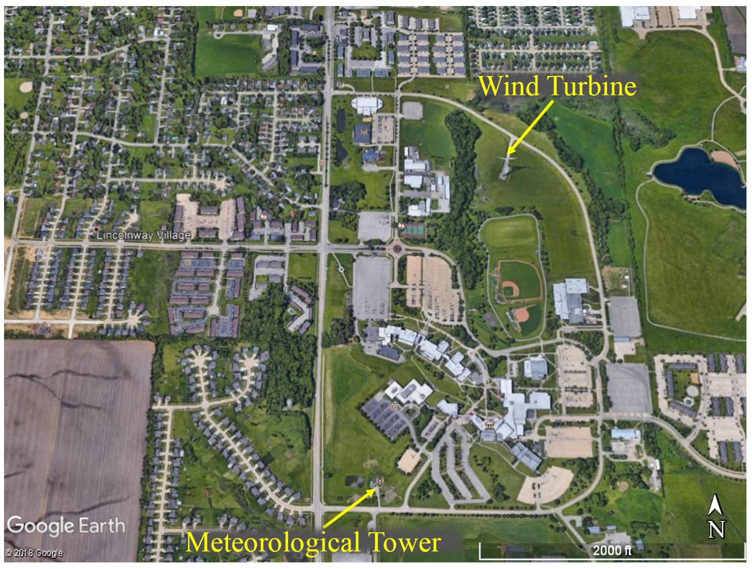
In the one-second version of the model, high frequency data are needed to correct the inflow in terms of yaw error, however, in practice, SCADA date are recorded as ten-minute average and standard deviation, therefore, high frequency data are seldom available. For this reason, an equivalent wind speed is generated using ten-minute mean and standard deviation of data, in this model, similar to the approach used in [8].

To obtain the rotor normal component of wind speed in Equation (3), we first apply Reynolds decomposition to density corrected wind speed and yaw error and we get:

$$U_{\rho }=\overline{U_{\rho }}(t,z)+{U_{\rho }}^{\prime }(t,z),$$

(11)

$$\theta (t,z)=\overline{\theta }(t,z)+{\theta }^{\prime }(t,z),$$

(12)

and the following approximation is applied:

$$\cos \theta =1-{\displaystyle \frac{{\theta }^2}{2}}.$$

(13)

Substituting Equation (13) into Equation (3), applying Reynolds averaging on $U_{\rho n}$, and neglecting high order terms, the mean and variance of $U_{\rho n}$ become:

$$\overline{U_{\rho n}}\approx \overline{U_{\rho }}-{\displaystyle \frac{\overline{U_{\rho }}{\overline{\theta }}^2}{2}}-{\displaystyle \frac{\overline{U_{\rho }}{\sigma }_{\theta }^2}{2}},$$

(14)

and

$$\overline{{U_{\rho n}}^{{\prime }^2}}\approx ({\sigma }_{u_{\rho }}^2+{\displaystyle \frac{{\sigma }_{u_{\rho }}^2{\overline{\theta }}^4}{4}}-{\sigma }_{u_{\rho }}^2{\overline{\theta }}^2+{\overline{U_{\rho }}}^2{\overline{\theta }}^2{\sigma }_{\theta }^2-{\displaystyle \frac{{\overline{U_{\rho }}}^2{\sigma }_{\theta }^2{\sigma }_{\theta }^2}{4}}).$$

(15)

Substituting Equations (14) and (15) into Equation (7) yields:

$$\overline{P}(t,z)={\displaystyle \frac{1}{2}}{\rho }_0{C}_{p}A[{(\overline{U_{\rho }}-{\displaystyle \frac{\overline{U_{\rho }}{\overline{\theta }}^2}{2}}-{\displaystyle \frac{\overline{U_{\rho }}{\sigma }_{\theta }^2}{2}})}^3+3(\overline{U_{\rho }}-{\displaystyle \frac{\overline{U_{\rho }}{\overline{\theta }}^2}{2}}-{\displaystyle \frac{\overline{U_{\rho }}{\sigma }_{\theta }^2}{2}})({\sigma }_{u_{\rho }}^2+{\displaystyle \frac{{\sigma }_{u_{\rho }}^2{\overline{\theta }}^4}{4}}-{\sigma }_{u_{\rho }}^2{\overline{\theta }}^2+{\overline{U_{\rho }}}^2{\overline{\theta }}^2{\sigma }_{\theta }^2-{\displaystyle \frac{{\overline{U_{\rho }}}^2{\sigma }_{\theta }^2{\sigma }_{\theta }^2}{4}})].$$

(16)

Applying the equivalent wind speed framework we get:

$${U_{eq}}_{10}\left(z\right)=\sqrt[3]{{(\overline{U_{\rho }}-{\displaystyle \frac{\overline{U_{\rho }}{\overline{\theta }}^2}{2}}-{\displaystyle \frac{\overline{U_{\rho }}{\sigma }_{\theta }^2}{2}})}^3+3(\overline{U_{\rho }}-{\displaystyle \frac{\overline{U_{\rho }}{\overline{\theta }}^2}{2}}-{\displaystyle \frac{\overline{U_{\rho }}{\sigma }_{\theta }^2}{2}})({\sigma }_{u_{\rho }}^2+{\displaystyle \frac{{\sigma }_{u_{\rho }}^2{\overline{\theta }}^4}{4}}-{\sigma }_{u_{\rho }}^2{\overline{\theta }}^2+{\overline{U_{\rho }}}^2{\overline{\theta }}^2{\sigma }_{\theta }^2-{\displaystyle \frac{{\overline{U_{\rho }}}^2{\sigma }_{\theta }^2{\sigma }_{\theta }^2}{4}})},$$

(17)

as a function of ten-minute SCADA statistics. Similar to Equation (9), ${U_{eq}}_{10}$ at each height where wind speed is measured, is integrated vertically considering the section of the rotor swept area it represents. The resulting variable is a ten-minute rotor equivalent wind speed:

$${U_{req}}_{10}={\displaystyle \frac{1}{A}}\sum _i{A}_i{U_{eq10}}_{i}i=1,2,\dots ,n.$$

(18)

The resulting time-averaged power can be expressed as:

$$\overline{P}={\displaystyle \frac{1}{2}}{\rho }_0{C}_{p}A{{U_{req}}_{10}}^3.$$

(19)

Subscript 10 in Equations (18) and (19) denotes that equivalent wind speeds and rotor equivalent wind speed are calculated using ten-minute data. The main difference between ${U_{req}}_{10}$ and ${U_{req}}_s$ is that ${U_{req}}_s$ is computed directly from data measured at 1 Hz rate, while ${U_{req}}_{10}$ is the same variable, but approximated based on ten-minute data.

3. Data Description

The data used in this study were collected from the site of a stand-alone wind turbine located on the northeastern side of Kirkwood community college campus in Cedar Rapids, Iowa. The wind turbine was built in 2012 and generates power for the campus. There is also a tall meteorological evaluation tower (met tower) located at a distance of 900 m south of the wind turbine. The met tower is used to characterize the atmospheric boundary layer (ABL) conditions at the site. Data from a period of approximately four months—from 20 February to 18 June 2018—were used in this study. More information about this site can be found in [19].

3.1. Turbine Data

The studied wind turbine is a Clipper Liberty 2.5 MW turbine, which is a three-bladed, horizontal axis wind turbine. It is a pitch-regulated wind turbine with a hub height of 80 m and a rotor diameter of 96 m. The turbine was downgraded to 2.3 MW by the operator to reduce maintenance costs. The lower tip of the rotor is approximately at a height of 32 m and the upper tip is at 128 m. It has a cut-in wind speed of 4 m·s⁻¹ and reaches its rated power at 13.5 m·s⁻¹ (Figure 1). The SCADA system of the turbine provides the standard ten-minute averaged wind speed, temperature, pressure, turbine orientation, power generation and wind turbine operational data. A unique feature of this site is storage of SCADA data from the turbine at 1 Hz rate, a feature that allows us to implement both variations of the model and study the effect of averaging timescale on the performance of the model.

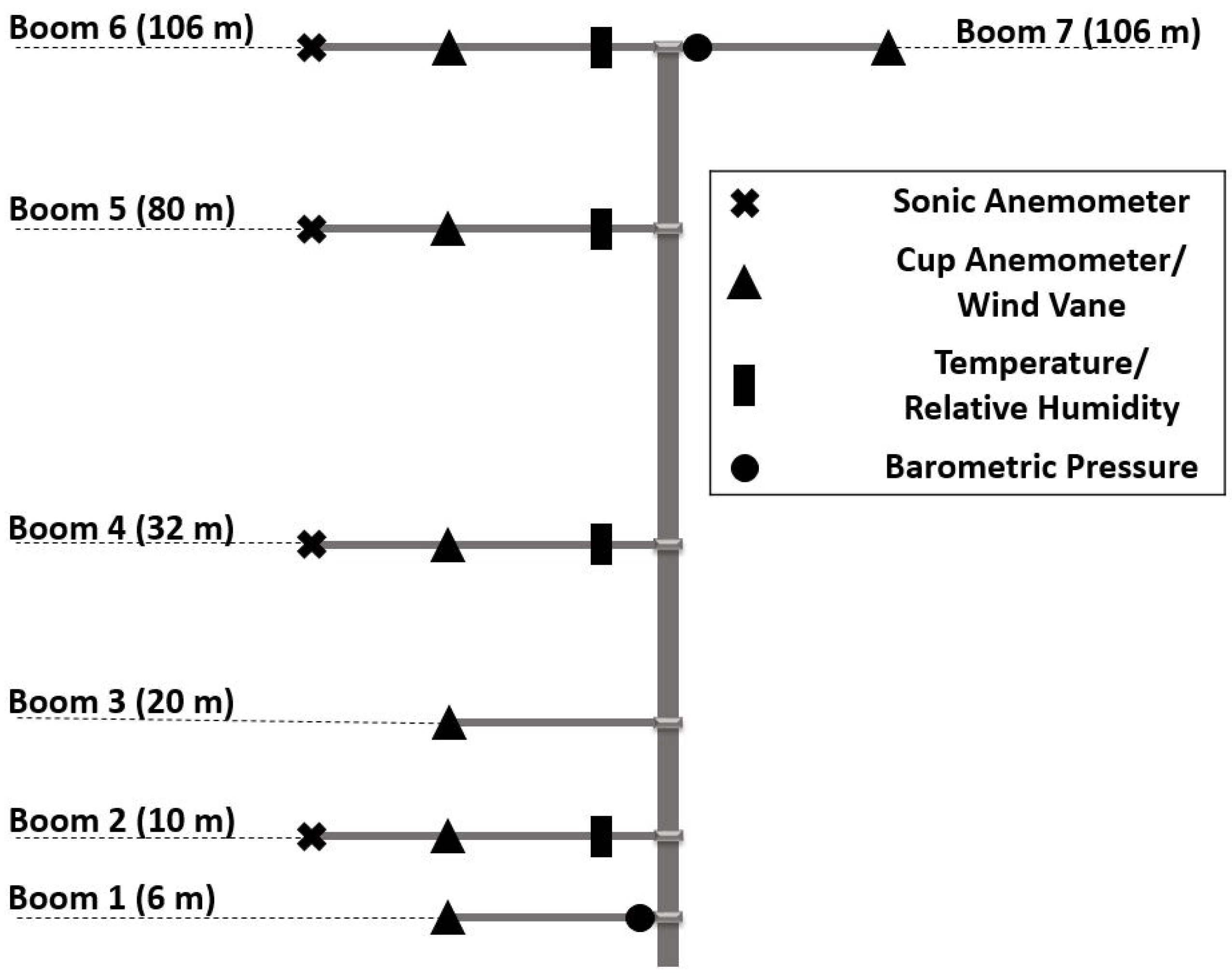
3.2. Meteorological Tower Data

In August 2017, a 106 m tall meteorological tower on the southwestern side of the campus was instrumented at several heights in order to characterize the atmospheric boundary layer near the turbine.

Table 1. List of instruments on the met tower.

Sensor	Make/Model	Quantity	Heights	Resolution
Barometric Pressure	Setra 278	2	6, 106 m	1 Hz
Temperature Sensor	NRG 110S	2	6, 20 m	1 Hz
Wind Vane	NRG 200P	7	6, 10, 20, 32, 80, 106 m	1 Hz
Cup Anemometer	A100LK	7	6, 10, 20, 32, 80, 106 m	1 Hz
T/RH Sensor	Vaisala-HMP 155	4	10, 32, 80, 106 m	1 Hz
Sonic Anemometer	Campbell Scientific-CSAT3B	4	10, 32, 80, 106 m	20 Hz
Gas Analyzer	LICOR-LI 7500-RS	1	106 m	20 Hz
Gas Analyzer	Campbell Scientific-Irgason	1	106 m	20 Hz
Radiometer	Kipp&Zonen-CNR4	1	106 m	1 Hz

provides a list of all sensors on the met tower. These sensors are mounted on seven booms at six different heights, with two booms on top of the tower oriented in opposite directions.

Relative location of the met tower with respect to the wind turbine is shown in Figure 3, which shows complexities of the terrain at this site. Generally, the structures surrounding both the wind turbine and the met tower are similar in the northwest and west direction. However, the Kirkwwod community college campus, located on the south side of the turbine, could affect the wind flow at the turbine, therefore, measurements collected at this site need to be analyzed carefully. More details about quality checks performed on the data are provided in Section 3.3.

Figure 4 shows a schematic of the met tower with a list of the sensors mounted on each of the seven booms. Four of the booms have sonic anemometers mounted on them, hence they are 21 feet and longer than the other booms which are 12 feet. Booms 1–6 extend westerly while boom 7 extends easterly. Boom 4 (32 m) is aligned with the lower tip of the rotor, boom 5 (80 m) is aligned with hub height and boom 6 (106 m) is at the top of the tower. Sonic anemometers, temperature/relative humidity sensors and wind vanes at 32 m, 80 m and 106 m are used in this study to characterize the inflow wind profile and is discussed in the following sections.

3.3. Data Quality Control

3.3.1. Meteorological Tower Data

Data from the met tower sensors were quality checked based on several criteria and measurements that do not pass the quality tests were discarded. Non-ideal conditions such as rainfall result in inaccurate measurement of wind by sonic anemometers, thus data collected under such conditions were flagged and removed from the analysis. Furthermore, measurements that exceed the limits of the instrument provided by manufacturer were flagged as well. Spike detection was another quality check performed on the data. Spikes were defined as excessively large fluctuations that can result from random sensor malfunction. Data points that exceed five times the standard deviation during a 30-minute window were considered as spikes in this study [21,22,23]. After removing flagged data points according to these criteria, any averaging window in which 5% or more of its data had been flagged was also removed, as suggested by St Martin et al. [9]. The combination of these quality checks resulted in removing approximately 10% of the data (1800 ten-minute data points removed).

Because data from the met tower are used to characterize the inflow into the turbine, met tower data should accurately represent flow conditions at the location of the turbine. However, the complex terrain at this site and different structures surrounding the wind turbine and the met tower do not allow us to solely rely on met tower measurement. Moreover, nacelle measurements need to be corrected to represent free flow according to IEC [20], therefore, a combination of measurements from the met tower and the nacelle were used after several quality checks were performed on the data.

Figure 5 Shows wind roses from ten-minute averaged SCADA and met tower data with predominant winds from the east, south and northwest. However, because wind directions that place the met tower at the wake of the turbine would result in inaccurate inflow characterization, met tower data that include northeasterly winds were removed from the dataset. Moreover, the topography of the turbine site causes negative shear when the wind blows from the north. Neither case was considered in this study by removing winds blowing from 340° to 90°. These criteria result in removing 40% of the data (7350 ten-minute data points).

Moreover, different landscapes and structures surrounding the met tower and the wind turbine, especially on the south, affect the wind profile at this site. This means the inflow at the met tower and the inflow at the wind turbine are not the same at all times, and the data needed to be filtered carefully. Smith et al. [24] compared data from nacelle anemometers and met towers at three different locations and reported little difference in power prediction based on met tower data and nacelle data. Similarly, in this study, ten-minute met tower data at hub height were compared to data from SCADA, and data points that result in a 10% difference or more between the two measurements were removed. A 10% threshold resulted in a coefficient of correlation between the two wind speed measurements similar to the ones reported in [24].

Figure 6 shows ten-minute averaged hub height wind speed and wind direction measurements both from SCADA and the met tower after above filters were applied. As it can be seen, after applying these filters, remaining data points are close to the diagonal line representing a 1:1 relationship between hub height wind speeds and directions at tower and turbine with an average of 0.35 m·s⁻¹ difference in wind speed measurement and an average of 6.6 degrees in wind direction measurement.

3.3.2. SCADA Data

SCADA data analysis revealed a significant number of data points where the turbine power generation is far from manufacturer provided power curve. St Martin et al. [9] explored two different ways to identify periods during which a turbine performance does not follow the power curve. Comparing blade pitch angle versus turbine operational parameters, they showed that the latter method results in losing fewer data, so this approach was used in this study as well. At this site, operators change the rated power limit of the turbine, thus all ten-minute periods during which rated power of the turbine is set below 2.3 MW were removed in this study. Other situations that affect data collection included periods when the grid is not in operational range, when the turbine is not operational due to being serviced, or when the generator is not operational. These criteria resulted in removing 27% of the data (5165 ten-minute data points). In total, after applying all quality checks, 77% of the data (14,315 ten-minute data points) were removed.

4. Discussion of Results

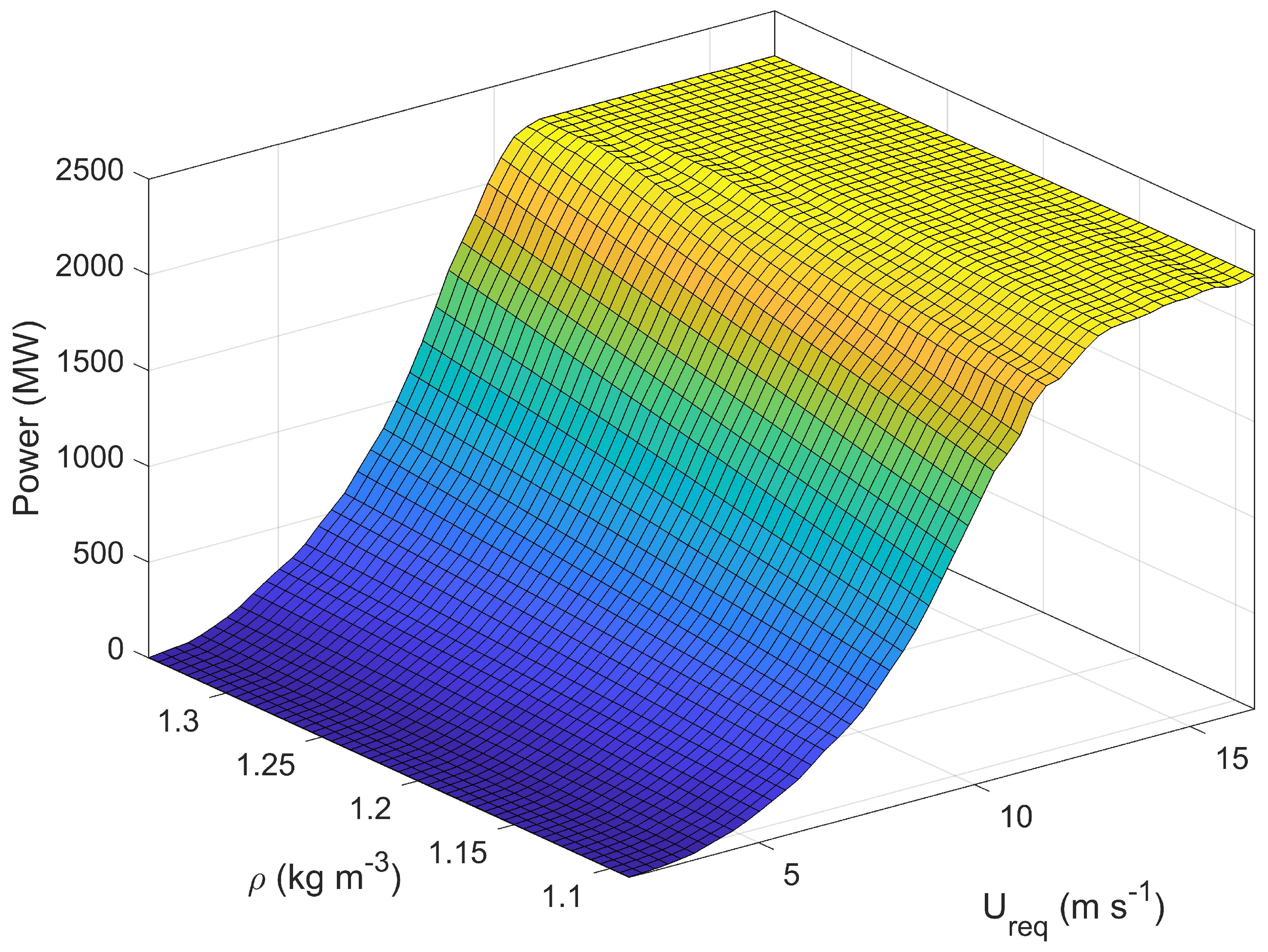
The two modified power curves were generated, their performance was compared to standard power curves and finally a power surface was proposed and its performance was examined. First, quality checks explained in the previous section were applied to the data and data points that pass theses quality checks were used in the model for wind turbine power prediction. Figure 7 shows that meteorological variables at this site, such as air density, turbulence intensity, wind shear, and wind veer vary significantly. Because of this variation, it was necessary to include these meteorological variables into the prediction model to improve the accuracy of power prediction.

Figure 7a shows the distribution of hub height wind speed; this distribution resembles a normal distribution with a mean wind speed of 7.8 m·s⁻¹ for the four month period of study. It should be noted that average wind speed during the period of study is higher than annual average wind speed at the site [19]. Turbulence is also important for predicting wind turbine power. A typical measure of turbulence at the turbine inflow is turbulence intensity ($TI$), defined as follows [17]:

$$TI={\displaystyle \frac{{\sigma }_U}{U}}.$$

(20)

Figure 7b shows the distribution of turbulence intensity at hub height. Closer inspection of the data revealed that wind speed at different measured heights can vary considerably, therefore inclusion of vertical shear effect on power production is important at this site. Figure 7c shows the distribution of shear exponent $\alpha$ for the power law profile of wind speed [17]:

$$U\left(z\right)=\beta z^{\alpha },$$

(21)

where z is height above the ground and $U\left(z\right)$ is the corresponding ten-minute average wind speed. Data from three sonic anemometers at heights 32 m, 80 m and 106 m were used to estimate the shear exponent, because these anemometers represent the rotor swept area. Furthermore, we assumed that the mean shear at the wind turbine is the same as the shear measured at the met tower and therefore the shear exponent is the same. It should be noted that this assumption was not true at all times, due to the effect of surrounding structures on the incoming flow. However, we only considered periods during which the flow conditions are close at the met tower and the wind turbine, as shown in Figure 6.

Besides wind shear variability, data from the site also reveal considerable variability in wind direction with height. To quantify wind direction variability, wind direction data at heights 32 m, 80 m and 106 m were used. For each ten-minute period, standard deviation of wind direction at these three heights was used to characterize wind veer [25]. Figure 7d shows distribution of wind veer at this site and it can be seen that the mean value of wind veer was around 6 degrees, even though it remains less than 10 degrees 90% of the time. In our model, the effect of wind veer is accounted for by using yaw error for correcting wind speed at each measured height (Equation (3)) and integrating the results vertically.

Another important meteorological variable that affects wind turbine power generation is air density. Air density is linearly related to power production and its effect is accounted for by adjusting wind speed for density variations in Equation (2). In this equation, a reference density (${\rho }_0$ = 1.225 kg·m⁻³) is used to normalize air density variations. Ambient pressure, temperature, and relative humidity measurements were used for calculating air density at hub height. The distribution is shown in Figure 7e. As it can be seen, air density at this site varies considerably with a mean value of 1.19 kg·m⁻³ during the four-month period of study, which is close to the reference density.

As mentioned above, including meteorological variables such as air density, turbulence intensity, wind shear and wind veer, improves power prediction. Equations (9) and (18) provide two different rotor equivalent wind speeds that take into account the effect of these meteorological variables. The same bin-averaging method used for generating the current industry standard power curves can be used to generate modified power curves from the rotor equivalent winds speeds. Figure 8 shows three resulting power curves. It should be noted that the x-axis is different for these curves; for standard power curves the x-axis represents wind speed while in the other two curves, the x-axis represents the respective equivalent wind speed. The standard power curve falls below both modified power curves, due to the fact that rotor equivalent wind speeds only take into account the normal component of wind speed, which is smaller than total wind speed. They also represent the whole rotor swept area, and lower wind speeds at lower heights result in rotor equivalent wind speeds being smaller than hub height wind speed.

The power curves in Figure 8 were used to estimate power generation, and training error was considered as a measure of accuracy for them. In other words, the dataset spanning from 20 February to 18 June 2018 was analyzed to fit these power curves (to train the model), and these curves were used to predict power during the same period. The difference between predicted and actual power generation is called training error. For quantifying training error, root mean square error ($RMSE$) and mean absolute error ($MAE$) were considered, defined as follow:

$$RMSE=\sqrt{{\displaystyle \frac{1}{n}}\sum _{i=1}^n{(P_i-{\widehat{p}}_i)}^2},$$

(22)

$$MAE={\displaystyle \frac{1}{n}}\sum _{i=1}^n|P_i-{\widehat{p}}_i|,$$

(23)

where $P_i$ is the actual power and ${\widehat{p}}_i$ is the predicted power. Lower $RMSE$ and $MAE$ indicate more accurate power prediction. The two above measures have been previously used for quantifying accuracy of prediction models and represent expected error associated with each predicted data point [1]. Figure 9 shows the performance of the three discussed models in power prediction. Actual power is plotted on the x-axis, while predicted power is plotted on the y-axis. The diagonal shows a 1:1 relation, representing the ideal prediction; the more a model deviates from the diagonal, the more error. The color bar represents turbulence intensity. From Figure 9, we can deduce that all models tend to under-predict power production in high turbulence intensity cases, while they tend to over-predict low turbulence intensity cases. This error tells us that turbulence intensity has a systematic effect on power generation in all three models. Both modified power curves result in a higher accuracy in power prediction, however the systematic behavior of turbulence intensity is still apparent in both of them, which suggests further investigation is needed on the effect of turbulence. Figure 9a shows the performance of standard power curve, which results in $RMSE$ = 118 kW and $MAE$ = 87 kW. Figure 9b,c show the performance of the ten-minute and one-second versions of the model, both of which perform better than standard power curve with lower $RMSE$ and $MAE$. It is also apparent from the plots that the amount of scatter among the data points is decreased in both versions of the modified model and all data points are closer to the diagonal. In the ten-minute version of the model, $RMSE$ is decreased to 89 kW and $MAE$ is decreased to 64 kW, which is a 24% improvement in prediction in terms of both $RMSE$ and $MAE$. The one-second version results in $RMSE$ = 87 kW and $MAE$ = 63 kW, a 26% improvement in prediction of power compared to standard power curve, therefore there is only a slight improvement compared to the ten-minute version of the modified model. From this point forward, we focus on the ten-minute version of the model since it requires fewer data, and results in a similar accuracy in prediction.

Taking a closer look at Equation (2) reveals an additional problem. The choice of reference density in both standard and modified power curves affects power prediction. This is because the specific value considered for the reference density affects the final distribution of $U_{req}$, while the distribution of power remains the same. Therefore, the value of reference density affects the final prediction accuracy of the model. Figure 10 shows how the distribution of rotor equivalent wind speed changes for different values of reference density from 0.5 kg·m⁻³ to 2 kg·m⁻³, which is an exaggerated range of density variation, and did not happen during the period analyzed. The smaller is the value of reference density, the wider is the peak of the distribution. A chosen value of ${\rho }_0$ = 0.5 kg·m⁻³ results in the widest peak, while a chosen value of ${\rho }_0$ = 2 kg m⁻³ results in the narrowest peak in the distribution. The mean value of density at this site for the four month period of study is 1.19 kg·m⁻³, and the resulting distribution falls somewhere in between the widest and narrowest distributions.

Changes in the distribution of $U_{req}$, result in a change in the prediction accuracy of the model. Figure 11 shows how $RMSE$ and $MAE$ of the model change for different values of reference density. The optimum value for reference density was found to be ${\rho }_0$ = 1.19 kg·m⁻³, which coincides with the mean value of density over the whole four-month period of study and it is in agreement with IEC recommendation for generating power curves [16]. This value for reference density results in the lowest values of $RMSE$ = 86 kW and $MAE$ = 63 kW.

By setting the reference density to ${\rho }_0$ = 1.19 kg·m⁻³, we found the best performance of the model, as shown in Figure 12, compared to the standard power curve. Using the optimum value for reference density, the ten-minute version of the model achieves a 26% improvement in prediction in terms of both $RMSE$ and $MAE$ compared to standard power curve.

Power Surface

As discussed in the previous section, using a reference value for density normalization results in an optimization problem. In other words, the value of reference density needs to be optimized for the dataset on which the power curve is based. To avoid this problem, we propose using a power surface by fitting a surface to the binned data instead of a curve. For that purpose, we need to use a two-dimensional bin averaging procedure based on wind speed and density as two independent variables. For this, a new formulation for rotor equivalent wind speed and associated power is developed as follows:

$$U_n(t,z)=U(t,z)\cos \left(\theta \right),$$

(24)

$$P(t,z)={\displaystyle \frac{1}{2}}\rho C_p{A}_i{U}_n{(t,z)}^3.$$

(25)

Following the same steps as Equations (11)–(18) yields:

$$U_{eq}\left(z\right)=\sqrt[3]{{(\overline{U}-{\displaystyle \frac{\overline{U}{\overline{\theta }}^2}{2}}-{\displaystyle \frac{\overline{U}{\sigma }_{\theta }^2}{2}})}^3+3(\overline{U}-{\displaystyle \frac{\overline{U}{\overline{\theta }}^2}{2}}-{\displaystyle \frac{\overline{U}{\sigma }_{\theta }^2}{2}})({\sigma }_U^2+{\displaystyle \frac{{\sigma }_U^2{\overline{\theta }}^4}{4}}-{\sigma }_U^2{\overline{\theta }}^2+{\overline{U}}^2{\overline{\theta }}^2{\sigma }_{\theta }^2-{\displaystyle \frac{{\overline{U}}^2{\sigma }_{\theta }^2{\sigma }_{\theta }^2}{4}})}.$$

(26)

The only difference between Equations (26) and (18) is that, in Equation (26), none of the velocity terms are normalized by density. Integrating the new equivalent wind speed vertically, considering the section of rotor swept area each measured height represents, results in:

$$U_{req}={\displaystyle \frac{1}{A}}\sum _i{A}_i{U_{eq}}_{i}i=1,2,\dots ,n$$

(27)

$$\overline{P}={\displaystyle \frac{1}{2}}\rho C_{p}A{U_{req}}^3.$$

(28)

In Equation (28), we assume that density variations over ten-minute periods are negligible. Therefore, wind turbine generated power is a function of $\rho$ and $U_{req}$ and can be binned in a two-dimensional feature space.

Figure 13a shows the two-dimensional binning of wind power in terms of $\rho$ and $U_{req}$. The bin width along the $U_{req}$ axis is chosen to be 0.5 m·s⁻¹ according to IEC [16]. To have roughly equal number of bins along the $\rho$ axis, the bin width along this axis is set to be 0.01 kg·m⁻³. Available data are transferred onto two-dimensional bins and generated power is averaged over each bin as shown in Figure 13a. Because the available data do not cover the whole area of feature space, wind power is linearly interpolated along the $\rho$ axis to fill the whole feature space, as shown in Figure 13b. Then, interpolated two-dimensional binned date are used to create a three-dimensional power surface, as shown in Figure 14.

The power surface in Figure 14 can be used to predict wind power similar to standard power curves. Figure 15 compares the performance of the standard power curve, ten-minute version of the model, and the power surface. The standard power curve is generated based on IEC standard method [16]. We can conclude that the power surface produces the best results in terms of $RMSE$ and $MAE$, with a 38% improvement in $RMSE$ and a 39% improvement in $MAE$ compared to the standard power curve. The power surface performs even better than the ten-minute version of the model with the optimum value for reference density, with a 16% improvement in $RMSE$ and a 17% improvement in $MAE$.

5. Conclusions and Future Work

In this study, four months of data, from February 20 February to 18 June 2018, measured at a met tower and SCADA were used to develop three modified models for prediction of power from a 2.5 MW wind turbine: a ten-minute model, a one-second model and a power surface. The developed models incorporate the effects of turbulence, density, wind shear, and wind veer into the standard power curves in order to achieve better accuracy. A unique feature of the dataset from this site is the availability of one-second data from SCADA, which was used in the one-second model. Because SCADA is typically limited to ten-minute averaged data, only ten-minute date are used in the power surface and the ten-minute version of the modified curve.

Because of the complex nature of this site and the fact that the wind turbine and the met tower are surrounded by different landscapes and structures, full characterization of the ABL is not possible and we could not solely rely on measurements from the met tower or SCADA. Therefore, quality checks were performed on the data from the met tower and SCADA and only periods with acceptable quality based on strict criteria were used in the models. Power prediction from all three models were compared with the standard power curve in terms of $MAE$ and $RMSE$. The results show that all three models perform better than the standard power curve, while the power surface, which accounts for variable air density results in the most accurate prediction of power. When compared to standard power curves, the ten-minute and one-second versions of the model result in 24% and 26% improvement in power prediction accuracy, respectively, while the power surface results in a 38% improvement in power prediction accuracy. Furthermore, the improvement in power prediction accuracy will be more tangible when annual power generation is considered. Taking the four-month period of study in this work, $RMSE$ in predicting power generation decreases by 46 kW. Applying this estimate to a whole year, the error in predicting Annual Energy Production (AEP) decreases by 402.96 megawatt-hours. For electricity at $30–60 [26] per megawatt-hour, this difference would be $12,089–24,178 for each turbine, every year.

The results also suggest that, even though the incorporation of turbulence intensity into the new models reduces prediction error, its effect on power generation is still not fully accounted for and needs to be further investigated. Moreover, the effect of thermal stability on the new models has not been studied yet. The new models need to be examined more carefully to understand how they perform under different stability regimes, in order to understand what stability variables need to be added to these models.

References

1. Clifton, A.; Kilcher, L.; Lundquist, J.; Fleming, P. Using machine learning to predict wind turbine power output. Environ.Res. Lett. 2013, 8, 024009. [Google Scholar] [CrossRef]
2. Wagner, R.; Courtney, M.; Gottschall, J.; Lindeløw-Marsden, P. Accounting for the speed shear in wind turbine power performance measurement. Wind Energy 2011, 14, 993–1004. [Google Scholar] [CrossRef]
3. Wagner, R.; Antoniou, I.; Pedersen, S.M.; Courtney, M.S.; Jørgensen, H.E. The influence of the wind speed profile on wind turbine performance measurements. Wind Energy 2009, 12, 348–362. [Google Scholar] [CrossRef]
4. Kaiser, K.; Langreder, W.; Hohlen, H.; Højstrup, J. Turbulence correction for power curves. In Wind Energy; Springer: Berlin/Heidelberg, Germany, 2007; pp. 159–162. [Google Scholar]
5. Langreder, W.; Kaiser, K.; Hohlen, H.; Hojstrup, J. Turbulence Correction for Power Curves; EWEC: London, UK, 2004. [Google Scholar]
6. Tindal, A.; Johnson, C.; LeBlanc, M.; Harman, K.; Rareshide, E.; Graves, A. Site-specific adjustments to wind turbine power curves. In Proceedings of the AWEA Wind Power Conference, Houston, TX, USA, 1–4 June 2008. [Google Scholar]
7. Albers, A.; Jakobi, T.; Rohden, R.; Stoltenjohannes, J. Influence of meteorological variables on measured wind turbine power curves. In Proceedings of the European Wind Energy Conference & Exhibition, Milan, Italy, 7–10 May 2007; pp. 525–546. [Google Scholar]
8. Choukulkar, A.; Pichugina, Y.; Clack, C.T.; Calhoun, R.; Banta, R.; Brewer, A.; Hardesty, M. A new formulation for rotor equivalent wind speed for wind resource assessment and wind power forecasting. Wind Energy 2016, 19, 1439–1452. [Google Scholar] [CrossRef]
9. St Martin, C.M.; Lundquist, J.K.; Clifton, A.; Poulos, G.S.; Schreck, S.J. Wind turbine power production and annual energy production depend on atmospheric stability and turbulence. Wind Energy Sci. 2016, 1, 221–236. [Google Scholar] [CrossRef]
10. Wharton, S.; Lundquist, J.K. Atmospheric stability affects wind turbine power collection. Environ. Res. Lett. 2012, 7, 014005. [Google Scholar] [CrossRef]
11. Redfern, S.; Olson, J.B.; Lundquist, J.K.; Clack, C.T. Incorporation of the Rotor-Equivalent Wind Speed into the Weather Research and Forecasting Model’s Wind Farm Parameterization. Mon. Weather Rev. 2019, 147, 1029–1046. [Google Scholar] [CrossRef]
12. Monterio, C.; Bessa, R.; Miranda, V.; Botterud, A.; Wang, J.; Conzelmann, G. Wind Power Forecasting: State-of-the-Art; Technical Report; Argonne National Laboratory: Argonne, IL, USA, 2009.
13. Li, S.; Wunsch, D.C.; O’Hair, E.A.; Giesselmann, M.G. Using neural networks to estimate wind turbine power generation. IEEE Trans. Energy Convers. 2001, 16, 276–282. [Google Scholar]
14. Jeon, J.; Taylor, J.W. Using conditional kernel density estimation for wind power density forecasting. J. Am. Stat. Assoc. 2012, 107, 66–79. [Google Scholar] [CrossRef]
15. Fugon, L.; Juban, J.; Kariniotakis, G. Data mining for wind power forecasting. In Proceedings of the European Wind Energy Conference & Exhibition EWEC 2008, Brussels, Belgium, 31 March–3 April 2008. [Google Scholar]
16. IEC. International Standard, Wind Turbines-Part 12-1: Power Performance Measurements of Electricity Producing Wind Turbines; IEC 61400-12-1; International Electrotechnical Commission: Geneva, Switzerland, 2005. [Google Scholar]
17. Burton, T.; Jenkins, N.; Sharpe, D.; Bossanyi, E. Wind Energy Handbook; John Wiley & Sons: Chichester, UK, 2011. [Google Scholar]
18. Shin, D.; Ko, K. Application of the Nacelle Transfer Function by a Nacelle-Mounted Light Detection and Ranging System to Wind Turbine Power Performance Measurement. Energies 2019, 12, 1087. [Google Scholar] [CrossRef]
19. Carbajo Fuertes, F.; Markfort, C.D.; Porté-Agel, F. Wind Turbine Wake Characterization with Nacelle-Mounted Wind Lidars for Analytical Wake Model Validation. Remote Sens. 2018, 10, 668. [Google Scholar] [CrossRef]
20. International Electrotechnical Commission. Power Performance of Electricity Producing Wind Turbines Based on Nacelle Anemometry; Technical Report, IEC 61400-12-2 CD Part 12-2; International Electrotechnical Commission: Geneva, Switzerland, 2008. [Google Scholar]
21. Mauder, M.; Foken, T. Documentation and Instruction Manual of the Eddy-Covariance Software Package TK3 (Update); University of Bayreuth: Bayreuth, Germany, 2015. [Google Scholar]
22. Lee, X.; Massman, W.; Law, B. Handbook of Micrometeorology: A Guide for Surface Flux Measurement and Analysis; Springer Science & Business Media: Dordrecht, The Netherlands, 2004; Volume 29. [Google Scholar]
23. Burba, G. Eddy Covariance Method for Scientific, Industrial, Agricultural And Regulatory Applications: A Field Book on Measuring Ecosystem Gas Exchange and Areal Emission Rates; LI-Cor Biosciences: Lincoln, NE, USA, 2012. [Google Scholar]
24. Smith, B.; Link, H.; Randall, G.; McCoy, T. Applicability of Nacelle Anemometer Measurements for Use in Turbine Power Performance Tests; Technical Report; National Renewable Energy Lab.: Golden, CO, USA, 2002.
25. Bulaevskaya, V.; Wharton, S.; Clifton, A.; Qualley, G.; Miller, W. Wind power curve modeling in complex terrain using statistical models. J. Renew. Sustain. Energy 2015, 7, 013103. [Google Scholar] [CrossRef]
26. Wiser, R.; Bolinger, M. 2010 Wind Technologies Market Report; Technical Report; National Renewable Energy Lab.: Golden, CO, USA, 2011.
Figure 1. Power curve for the 2.5 MW study turbine, derived using ten-minute data from 20 February to 18 June 2018 and bins of 1 m·s−1. Cut-in region, operational region and rated region are shown.
Energies 12 01805 g001
Figure 2. Wind veer and shear at inflow results in different values of yaw error ( θ ) and wind speed at different heights. Turbulence also causes fluctuations over mean values of wind speed, yaw error and density. All of these variables are used for predicting power generation by the wind turbine.
Energies 12 01805 g002
Figure 3. Location of wind turbine of study in relation to 106 m met tower. Kirkwood community college campus is located in between. Image: Google.
Energies 12 01805 g003
Figure 4. Mounting position of instruments and boom levels on the met tower. Booms 1–6 extend towards the west while boom 7 extends towards the east.
Energies 12 01805 g004
Figure 5. Wind rose at the site of the wind turbine from: (a) SCADA data; and (b) met tower data. Wind rose were generated after quality checks were applied to the data for the period of study.
Energies 12 01805 g005
Figure 6. Ten-minute averaged Hub height (a) wind speed and (b) wind direction measurements from SCADA and met tower data after preliminary quality checks. The dashed diagonal line shows a 1:1 relationship. It should be noted that wind direction at hub height from met tower was not available during the period of study due to sensor failure, and it was interpolated from wind direction at 32 m and 105 m.
Energies 12 01805 g006
Figure 7. The observed distribution of meteorological variables based on ten-minute averaged data: (a) hub height wind speed (m·s−1); (b) turbulence intensity (TI) at hub height; (c) shear exponent; (d) wind veer (degrees); and (e) air density at hub height (kg·m−3).
Energies 12 01805 g007aEnergies 12 01805 g007b
Figure 8. Standard power curve versus ten-minute and one-second versions of the model based on bins of 0.5 m·s−1 and ρ 0 = 1.225 kg·m−3.
Energies 12 01805 g008
Figure 9. Performance of: (a) standard power curve; (b) ten-minute version of the model; and (c) one-second version of the model, when a reference density of ρ 0 = 1.225 kg·m−3 is considered.
Energies 12 01805 g009
Figure 10. Distribution of rotor equivalent wind speed for three different values of ρ 0 . Smaller value of ρ 0 results in wider distribution of U r e q .
Energies 12 01805 g010
Figure 11. The effect of reference density on: (a) R M S E of the model; and (b) M A E of the model.
Energies 12 01805 g011
Figure 12. Performance of: (a) standard power curve; and (b) ten-minute version of the model, considering an optimum value for reference density ( ρ 0 = 1.19 kg·m−3).
Energies 12 01805 g012
Figure 13. (a) Two dimensional binning of wind power in terms of rotor equivalent wind speed and density using available data; and (b) linear interpolation of available data for filling empty bins. The bins’ dimensions are 0.5 m·s−1× 0.01 kg·m−3.
Energies 12 01805 g013
Figure 14. Power surface generated from interpolated binned data.
Energies 12 01805 g014
Figure 15. Performance of: (a) standard power curve with ( ρ 0 = 1.19 kg·m−3); (b) ten-minute modified power curve with ( ρ 0 = 1.19 kg·m−3); and (c) power surface.
Energies 12 01805 g015