A Novel Nonintrusive Load Monitoring Approach based on Linear-Chain Conditional Random Fields

Abstract

In a real interactive service system, a smart meter can only read the total amount of energy consumption rather than analyze the internal load components for users. Nonintrusive load monitoring (NILM), as a vital part of smart power utilization techniques, can provide load disaggregation information, which can be further used for optimal energy use. In our paper, we introduce a new method called linear-chain conditional random fields (CRFs) for NILM and combine two promising features: current signals and real power measurements. The proposed method relaxes the independent assumption and avoids the label bias problem. Case studies on two open datasets showed that the proposed method can efficiently identify multistate appliances and detect appliances that are not easily identified by other models.

1. Introduction

1.1. Background

As the core of an interactive service system, smart power utilization is one of the essential components of a smart grid. There are three aspects to the key technologies associated with this: advanced metering infrastructure (AMI) standards, systems, and terminal technologies; intelligent two-way interactive operation mode and supporting techniques; and the interaction between the user’s electrical environment and energy consumption patterns. In actual production, we must break through the bottleneck regarding the meter only being able to read the total amount of energy consumption rather than analyzing the internal load components for users. Load monitoring can not only improve the power information collection system and intelligent power system but also support two-way interactive service and smart power utilization. Nonintrusive load monitoring (NILM), which is a vital part of smart power utilization techniques, can achieve fine-grained tracking of energy consumption and provide load disaggregation information without any intrusive device installation. These data can be further applied to optimize energy conservation strategies.

1.2. Literature Review and Motivation

NILM was first proposed by Hart [1], who devised a method for appliance load monitoring by only identifying electrical appliances within the aggregate power consumption data. This method decomposes the aggregated data into the actual power components of each load and avoids cumbersome device installation. Since then, many new methods have been introduced for load disaggregation, such as Bayes [2] and support vector machines (SVMs) [3,4]. Bayes has shown good performance in some experiments. However, it requires the appliances to have stable power measurements, which is almost nonexistent in reality. Comparably, SVM performs better using low-frequency features. Chui [3] proposed a hybrid genetic algorithm support vector machine multiple kernel learning approach (GA-SVM-MKL), which solves the problems that current algorithms are limited by data granularity and consideration of fewer appliances. It has enhanced the performance indicators (sensitivity, specificity, and overall accuracy) up to 21% compared with traditional methods. Lai [4] used a hybrid SVM/GMM classifier that successfully achieved ubiquitous recognition service. In their model, GMM is employed to describe the distribution of the current measurement to find the power similarity, while SVM is applied to identify the appliances. However, an SVM method can be arbitrary given a large dataset and requires tedious training for best kernels and parameters.

The hidden Markov model (HMM) has become a mainstream algorithm, as it can include appliances’ state transition in its learning. Specifically, the task of NILM can be considered as assigning label sequences to a set of observation sequences. Thus, for a given set of aggregated load data, HMM-based approaches are naturally suitable for performing tasks such as identifying tags or disintegrating electrical loads. In previous works, HMM and its variants have improved the accuracy of NILM. Zia [5] applied an HMM-based method to identify personal devices and found that it can effectively distinguish the power consumption patterns of the appliances. Kong [6] proposed a hierarchical HMM (HHMM) framework for modeling household appliances, which provides a promising representation of devices with multiple built-in modes and different power consumption profiles. Kim [7] investigated the effectiveness of several unsupervised disaggregation methods and demonstrated that a conditional factorial hidden semi-Markov model performs better than other methods. Kolter [8] adopted factorial HMM and developed a convex formulation of approximate inference to make the inference algorithm computationally efficient and avoid the issues of local optima. Agyeman [9] came up with a variant of the HMM to identify loads and operation states by practicable measurable parameters. Their results show that the method can provide power usage information in a nonintrusive manner and is ideal for participation in the demand response market.

Nevertheless, the above models assume that any observation in the sequences is independent of the other [10]. In other words, the aggregated load data at any given time only depend on the states of loads at that time and have no association with previous ones. That is not appropriate for a realistic environment. The current data, such as the appliance power consumption, are highly relevant to an extended range of previous observations. There is a weakness in HMM-based models called the label bias problem [11]. When one state transitions to another, the Viterbi algorithm may choose the state with fewer outgoing transitions and takes little notice of the observations. Extraordinarily, the algorithm even ignores the observations if a state has a single outgoing transition. In this case, the result is highly relevant to the training set. If one state is slightly more common in the training set, the algorithm will prefer this transition, whatever the next observation may be.

Conditional random fields (CRFs) have also been used by Panikos [12] as an unsupervised model for energy disaggregation. They apply a clustering method and histogram analysis to detect the selected loads for residential users and have obtained higher-accuracy results compared with previous methods. However, they only detect the on/off states of devices and cannot handle multistate appliances. Additionally, CRFs can extract various features for training, but they only use power measurements as a feature, which may fail to make full use of the advantages of the CRF model.

In our paper, we have proposed a method called linear-chain CRFs for load disaggregation, which perfectly solves the above problems. Our linear-chain CRF model defines a log-linear distribution over all of the observation sequences in the aggregate data, which relaxes the requirements for the independence of observation data in HMM. It not only considers the influence of the previous state on the current state but can also incorporate all useful information in the observation, which makes it more viable in reality. Since CRFs define a log-linear distribution over all of the label sequences given in the observations, the transition metric between different state changes and the weights can be traded off. Thus, our linear-chain CRF model avoids the label bias problem. In addition, our model does not require the stable power measurements needed for Bayes as well as the exhausting parameter training needed for SVM. Moreover, by quantizing the power probability density function for each load, we can easily identify multistate appliances. We also employ two promising features: current signals and real power measurements to develop our model. Experimental results on two open datasets demonstrate that the proposed model is feasible for a NILM task.

1.3. Contributions

Our main contributions are as follow:

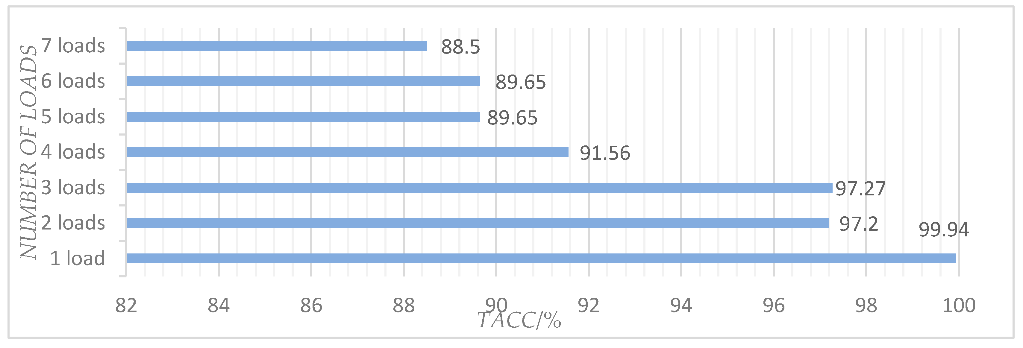
• We proposed a method called the linear-chain CRF model for load disaggregation and achieved accuracy of 96.04–99.94%. It is demonstrated that this method is effective for the NILM task.
• Because we relaxed the independent assumption required by HMM-based models and avoided the label bias problem, the performance is enhanced by 2.21% compared to existing models.
• We combined two promising features: current signals and real power measurements to build our model, which improved the accuracy of the model significantly.

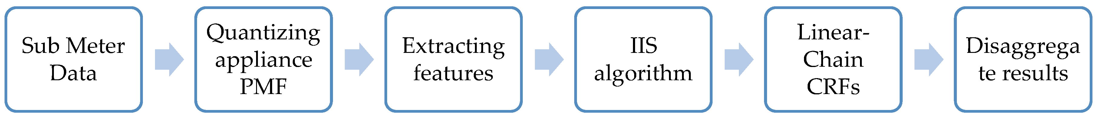
2. Methodology

Figure 1 shows the goal of our model: breaking down the aggregate data into the actual power consumption of each appliance. Figure 2 illustrates the main framework of our linear-chain CRF model for NILM. First, submeter data of each load was used to create the probability density function for each appliance to acquire the working states. Then, the states of the appliances were grouped to tag and segment the smart meter data. Next, our model extracted features over the training set according to the feature templates. Consequently, the improved iterative scaling algorithm (IIS) was used to train the linear-chain CRF model. Finally, we adopted the Viterbi algorithm to disaggregate the states for each appliance given the aggregate power data.

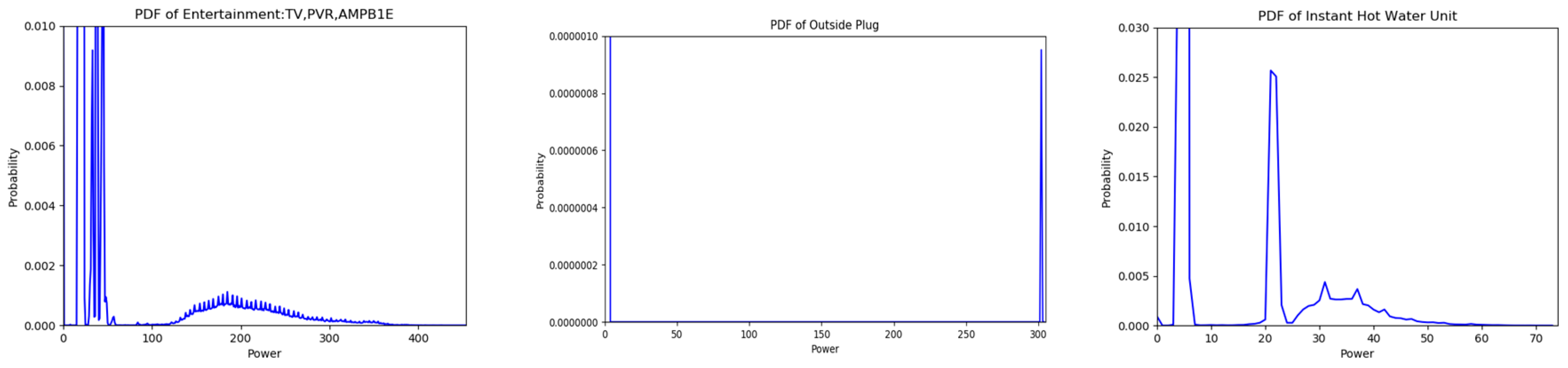
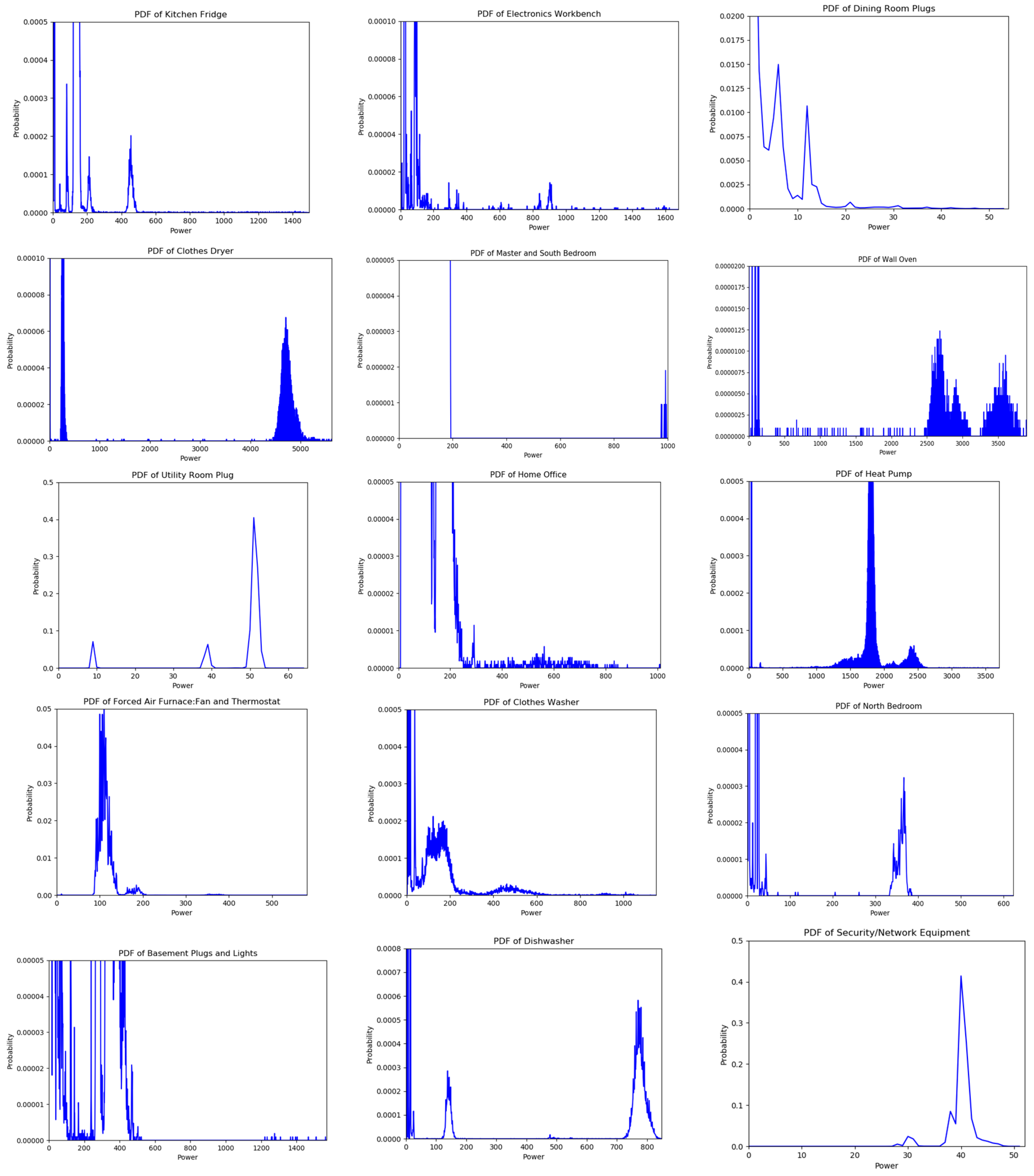
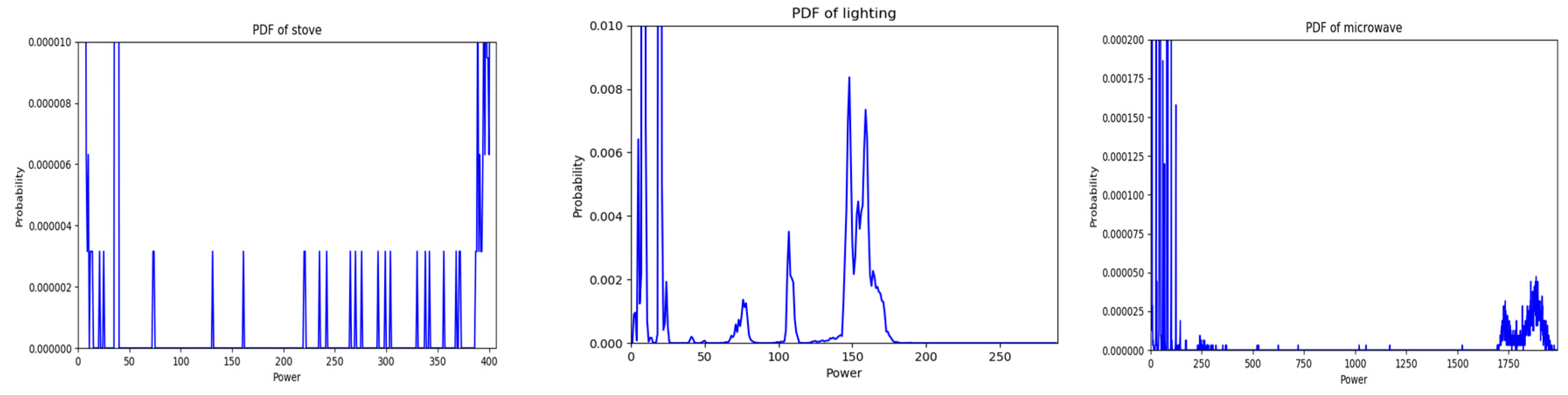
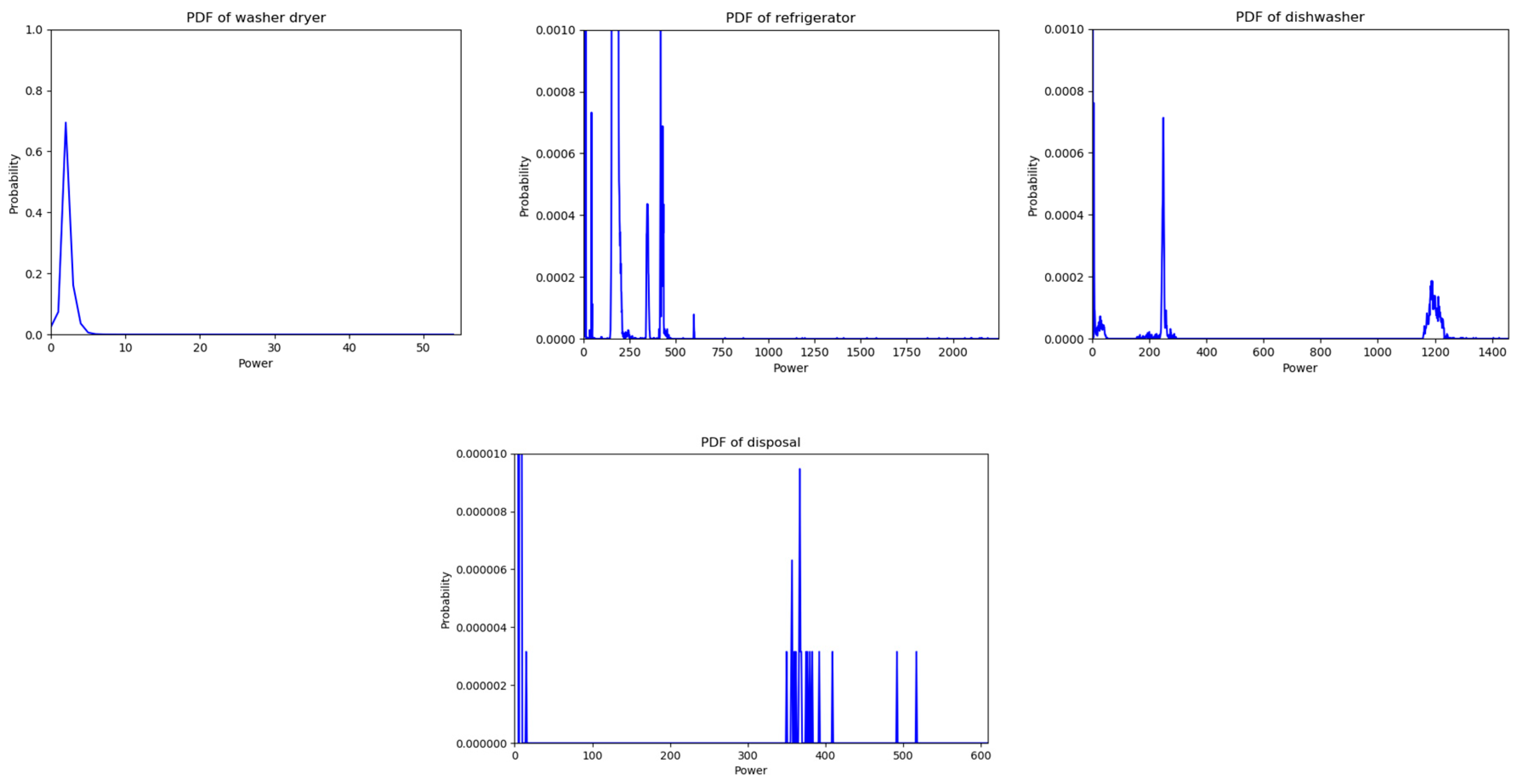
2.1. Probability Mass Functions

Various appliances, such as washing machines, have multiple operating states. The simple on state cannot reflect the real state change when the appliance is working. To identify the different working states of multistate type appliances at a given time, we used the approaches of Stephen [13] to quantize power probability mass function (PMF) for each appliance. We took the PMF as the probability density function (PDF) for their working states. Figure 3 and Figure 4 show the power PDF of some appliances in AMPds2 [14] and REDD house 2 [15]. Compared with low power measurements, most probabilities of high power measurements were excessively low, so we enlarged the y-axis scale appropriately to make it clear.

When the power measurement of the appliance is distributed in a certain power range, it indicates that the device is in a specific working state. By figuring out the power distribution and finding the power range of the concentrated power distribution, we could analyze the working states for appliances. Let $P\left(n\right)$ represent the probability of $n$, where $n$ is the number of possible observed power measurements. In Stephen’s [13] paper, they found the power range by capturing the peak, which is defined as when the slope on the left in the PDF is positive and the slope on the right is negative, which is to say:

$$P\left(n\right)-P\left(n-1\right)>0$$

(1)

$$P\left(n+1\right)-P\left(n\right)\le 0$$

(2)

$$P\left(n\right)>\epsilon =0.00021$$

(3)

where $\epsilon$ is used to make sure that the probabilities under this value will not be quantized as a state. However, on the one hand, we considered that the value of $\epsilon$ was hard to generalize since it varied in different datasets and different appliances. Furthermore, this method pays more attention to the peaks with higher probability. However, these peaks are mainly distributed in low power measurements, and most of them are noises rather than states. In fact, some high power measures include some major working states, to which importance should be attached. Therefore, we combined some states with low power measurements and concentrated on the states with high measurements according to the PDF of each appliance. On the other hand, this approach was used to identify a load with a finite number of operating states and that worked worse when the appliances belonged to continuously variable devices. It was apparent to see from the PDF that some appliances, such as dining room plugs and instant hot water units, were not multistate appliances. Thus, it was inapplicable to quantize their PDFs for working states. We simply determined the on/off states for this type of appliance. More details are discussed in Section 3.

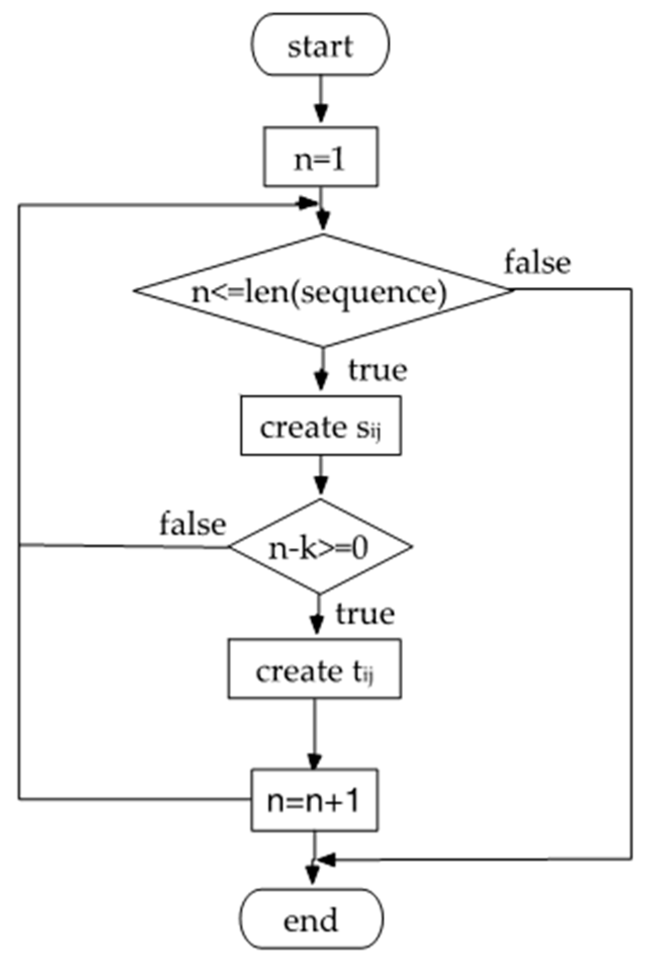
2.2. Segmenting Data

CRFs are a framework for segmenting and labeling sequential data. Let $S=\left\{s_1,s_2,\dots ,s_n\right\}$ be the label sequences, and $P=\left\{p_1,p_2,\dots ,p_n\right\}$ be the observation sequences. A graphical structure of linear-chain CRFs is shown in Figure 5, which demonstrates that the input of our model is a series of sequences. Our templates then extract features throughout each chain. Therefore, segmenting smart meter data is crucial for feature extraction and model performance. CRFs are adept at dealing with a sentence with no more than 20 tokens. Considering that the working state of an appliance from an hour or 30 min ago has little effect on the current working state, we segmented smart meter data into a sequence for the AMPds2 datasets every 10 min and every minute for the REDD dataset in terms of their different sampling rates (per minute in AMPds2 and per 3 s in REDD). Then, 10 tokens were included in a sequence for the AMPds2 datasets and 20 for the REDD dataset, which made our model perform more efficiently compared with other segmentation methods.

2.3. Extracting Features

Let $Y=\left\{y_1,y_2,\dots ,y_n\right\}$ be the label sequences, $X=\left\{x_1,x_2,\dots ,x_n\right\}$ be the observation sequences, $\lambda =\left\{{\lambda }_k\right\}\in R, \mu =\left\{{\mu }_k\right\} \in R$ be the parameter vectors, and $P\left(y|x\right)$ represent the linear-chain CRFs. Then, define the probability of marking a tag sequence $Y$ on a given observation sequence $X$ as follows [16]:

$$P\left(y|x\right)=\frac{1}{Z\left(X\right)}\mathit{exp}\left({\displaystyle \sum }_{i,k}{\lambda }_k{t}_k\left(y_{i-1},y_i,x,i\right)+{\displaystyle \sum }_{i,l}{\mu }_l{s}_l\left(y_i,x,i\right)\right)$$

(4)

$$Z\left(x\right)={\displaystyle \sum }_y\mathit{exp}\left({\displaystyle \sum }_{i,k}{\lambda }_k{t}_k\left(y_{i-1},y_i,x,i\right)+{\displaystyle \sum }_{i,l}{\mu }_l{s}_l\left(y_i,x,i\right)\right)$$

(5)

where $t_k$ is a transition feature function depending on the current state $i$ and previous state $i-1$ in the label sequence given the observation sequences; $s_l$ is a state feature function depending on the current state $i$ in the label sequence, which is also viewed as a local feature function; and $\lambda =\left\{{\lambda }_k\right\}\in R, \mu =\left\{{\mu }_k\right\} \in R$ are the parameter vectors, which index the weights of the corresponding $t_k$ and $s_l$ function and can be learned by our model.

We defined feature functions $t_k$ and $s_l$ using feature templates. A feature template has the form of a single state $S_n$ or some combination of current states and previous states $S_{n-k}\dots S_n$. For example, assume that we have a power measurement sequence: 1919, 1918, 1921, 106, 107, 105, 106, 2, 3, 1. The corresponding state sequence is: 2, 2, 2, 1, 1, 1, 1, 0, 0, 0. A single state $S_n$ template refers to series state functions $s_{nj}$, where $n$ is the position of the current token and $j$ is the number of appliance states. Let the current token be the fifth one; then, we define $s_{51}:$ if (state = 1 and power measurement = 107) return 1 or else return 0; $s_{52}$: if (state = 2 and power measurement = 107) return 1 else return 0; $s_{53}$: if (state = 0 and power measurement = 107) return 1 else return 0. Similarly, templates have the form of $S_{n-k}\dots S_n$, representing several transition functions $t_{nj}$ where $n$ is the position of the current token, $n-k$ is the position of the previous token, and $j$ is the number of appliance states. Let $k=1$; then, we construct functions as follows: $t_{51}:$ if (state = 1 and power measurements = 106, 107) return 1 else return 0; $t_{52}:$ if (state = 2 and power measurement = 106, 107) return 1 else return 0; $t_{53}:$ if (state = 0 and power measurement = 106, 107) return 1 else return 0. The whole process is shown in Figure 6.

Our model constructs $L*N$ feature functions according to the feature templates designed, where $L$ represents the number of output types, and $N$ represents the number of expanded features. In practice, many feature functions are constructed. For example, in our experiments, 4,704,668 feature functions were produced for five loads (CWE, DWE, FRE, HPE, and WOE) in AMPds2. The excessive feature functions increased the complexity of our model and made it difficult for subsequent training and testing. Actually, some measurements in the dataset were inaccurate or completely noisy, which made those feature functions considering these measurements unnecessary. We found that the frequency of these feature functions’ occurrence was much less than normal functions. Therefore, we ignored those functions with fewer than three occurrences, which reduced the complexity greatly.

2.4. Improved Iterative Scaling (IIS) Algorithm

Formulas (4) and (5) define the primary form of linear-chain CRFs. The parameters ${\lambda }_k$ and ${\mu }_l$ are the corresponding weights to be estimated from the training set. From Formula (4), we can easily discover that the definition of $P\left(y|x\right)$ is similar to a maximum entropy model. Actually, the CRF model is motivated by the principle of maximum entropy. Thus, we could apply the IIS algorithm of the maximum entropy model for parameter learning.

To simplify, let there be $M_1$ transition feature functions and $M_2$ state feature functions, $M=M_1+M_2$, defined as

$$f_k\left(y,x\right)=\{\begin{array}{c}{\displaystyle {\displaystyle \sum }_{i=1}^n}{t}_k\left(y_{i-1},y_i,x,i\right), k=1,2,\dots M_1\\ {\displaystyle {\displaystyle \sum }_{i=1}^n}{s}_l\left(y_i,x,i\right),k= M_1+l;l=1,2,\dots ,M_2\end{array}$$

(6)

$${\omega }_k=\{\begin{array}{cc}{\lambda }_k,\hfill & \hfill k=1,2,\dots M_1\\ {\mu }_l,\hfill & \hfill k=M_1+l;l=1,2,\dots ,M_2\end{array}$$

(7)

$$\omega ={\left({\omega }_1,{\omega }_2,\dots ,{\omega }_M\right)}^T$$

(8)

$$F\left(y,x\right)={\left(f_1\left(y,x\right),f_2\left(y,x\right),\dots ,f_3\left(y,x\right)\right)}^T.$$

(9)

Then, CRF can be normalized as a product of vector $\omega$ and $F\left(y,x\right)$:

$$P_w(y|x)=\frac{1}{Z_w\left(x\right)}\mathit{exp}\left(\omega \cdot F\left(y,x\right)\right)$$

(10)

$$Z_w\left(x\right)={\displaystyle \sum }_y\mathit{exp}\left(\omega \cdot F\left(y,x\right)\right).$$

(11)

Given the empirical distribution $\tilde{P}\left(x,y\right)$, the log-likelihood function $L_{\tilde{p}}\left(P_w\right)$ of conditional probability distribution $P(y|x)$ is defined as:

$$L_{\tilde{p}}\left(P_w\right)=log{\displaystyle \prod }_{x,y}P{(y|x)}^{\tilde{P}\left(x,y\right)}={\displaystyle \sum }_{x,y}\tilde{P}\left(x,y\right)logP(y|x)$$

(12)

When $P(y|x)$ is defined as (10), the log-likelihood function can be derived as followed:

$$\begin{array}{ll}{L}_{\tilde{p}}\left(P_w\right)=& {\displaystyle {\displaystyle \sum }_{x,y}}\tilde{P}\left(x,y\right)logP(y|x)={\displaystyle {\displaystyle \sum }_{x,y}}\tilde{P}\left(x,y\right)log{P}_w(y|x)\\ & ={\displaystyle {\displaystyle \sum }_{x,y}}[\tilde{P}\left(x,y\right)\omega \cdot F\left(y,x\right)-\tilde{P}\left(x,y\right)log{Z}_w(x)]\\ & ={\displaystyle {\displaystyle \sum }_{x,y}}[\tilde{P}\left(x,y\right){\displaystyle {\displaystyle \sum }_{k=1}^M}{\omega }_k{f}_k\left(y,x\right)-\tilde{P}\left(x,y\right)log{Z}_w(x)]\\ & ={\displaystyle {\displaystyle \sum }_{i=1}^N}{\displaystyle {\displaystyle \sum }_{k=1}^M}{\omega }_k{f}_k\left(y_i,x_i\right)-{\displaystyle {\displaystyle \sum }_{i=1}^N}{Z}_w\left(x_i\right)\end{array}$$

(13)

Assuming the current vector $\omega ={\left({\omega }_1,{\omega }_2,\dots ,{\omega }_M\right)}^T$, the IIS algorithm tries to find the best vector $\omega +\delta ={\left({\omega }_1+{\delta }_1,{\omega }_2+{\delta }_2,\dots ,{\omega }_M+{\delta }_M\right)}^T$, which increases the value of the log-likelihood function. According to Adam [16], the IIS algorithm finds out the increment vector $\delta ={\left({\delta }_1,{\delta }_2,\dots ,{\delta }_M\right)}^T$ by solving the renewal equation for transition feature Function (14) and state feature Function (15):

$${\displaystyle \sum }_{x,y}\tilde{P}\left(x\right)P(y|x){\displaystyle \sum }_{i=1}^{n+1}{t}_k\left(y_{i-1},y_i,x,i\right)exp\left({\delta }_{k}T\left(y,x\right)\right)=E_{\tilde{p}}\left[t_k\right]$$

(14)

where $k=1,2,\dots ,M_1$; $y_i$ and $y_{i-1}$ refer to the current and previous power measurements; $y$ depends on all states.

$${\displaystyle \sum }_{x,y}\tilde{P}\left(x\right)P(y|x){\displaystyle \sum }_{i=1}^n{s}_l\left(y_i,x,i\right)exp\left({\delta }_{k}T\left(y,x\right)\right)=E_{\tilde{p}}\left[s_l\right]$$

(15)

where $k= M_1+l;l=1,2,\dots ,M_2$, $T\left(y,x\right)$ is the summation of all feature functions:

$$T\left(y,x\right)={\displaystyle \sum }_k{f}_k\left(y,x\right).$$

(16)

The complete IIS algorithm is shown in Algorithm 1 below.

Algorithm 1. Improved iterative scaling algorithm.

1: for k ∈ (1, M)

2:  ωk = 0

3: repeat

4: for k ∈ (1, M)

5:   if k ∈ (1, M1)

6:    ${\delta }_k\to {\displaystyle \sum }_{x,y}\tilde{P}\left(x\right)P(y|x){{\displaystyle \sum }}_{i=1}^{n+1}{t}_k\left(y_{i-1},y_i,x,i\right)\exp \left({\delta }_{k}T\left(y,x\right)\right)=E_{\tilde{p}}\left[t_k\right]$

7:   if k ∈ (M1 + 1, M)

8:    ${\delta }_k\to {\displaystyle \sum }_{x,y}\tilde{P}\left(x\right)P(y|x){{\displaystyle \sum }}_{i=1}^n{s}_l\left(y_i,x,i\right)\exp \left({\delta }_{k}T\left(y,x\right)\right)=E_{\tilde{p}}\left[s_l\right]$

9: ωk ← ωk + δk

10: until ωk converge

2.5. Viterbi Algorithm

The Viterbi algorithm for CRF prediction is similar to the one for HMM. Assuming that the observation sequences are $\left\{x\right\}$, then the task of prophecy is to find the max probability of label sequences {$y^{*}$}:

$$\begin{gathered} y^{*}=\underset{y}{argmax}\left(P_w\left(y|x\right)\right) \\ =\underset{y}{argmax}\frac{1}{Z_w\left(x\right)}\mathit{exp}\left(\omega \cdot F\left(y,x\right)\right) \\ =\underset{y}{argmax}\mathit{exp}\left(\omega \cdot F\left(y,x\right)\right) \\ =\underset{y}{argmax}\left(\omega \cdot F\left(y,x\right)\right). \end{gathered}$$

(17)

Therefore, the prediction problem for CRF is converted to $\underset{y}{max}\left(\omega \cdot F\left(y,x\right)\right)$. The Viterbi algorithm is shown in Algorithm 2 below.

Algorithm 2. Viterbi algorithm for CRF prediction.

1: Step 1: initialization

2: for j ∈ (1, m)

3:  ${\delta }_1\left(j\right)=\omega \cdot F\left(y_0=start,y_1=j,x\right)$

4: Step 2: recursion

5: for i ∈ (2, n)

6:    ${\delta }_i\left(l\right)=\underset{1\le j\le m}{\mathit{max}}\left\{{\delta }_{i-1}\left(j\right)+\omega \cdot F\left(y_{i-1}=j,y_i=l,x\right)\right\}$

7:   ${\phi }_i\left(l\right)=\underset{1\le j\le m}{argmax}\left\{{\delta }_{i-1}\left(j\right)+\omega \cdot F\left(y_{i-1}=j,y_i=l,x\right)\right\}$

8:    l = 1, 2, ..., m

9: Step 3: terminate

10:    $\underset{y}{\mathit{max}}\left(\omega \cdot F\left(y,x\right)\right)=\underset{1\le j\le m}{\mathit{max}}{\delta }_n\left(j\right)$

11:    $y_n=\underset{1\le j\le m}{argmax}{\delta }_n\left(j\right)$

12: Step 4: traceback

13: for i ∈ (n − 1, 1)

14:    $y_i={\phi }_{i+1}\left(y_{i+1}\right)$

3. Experiment and Analysis

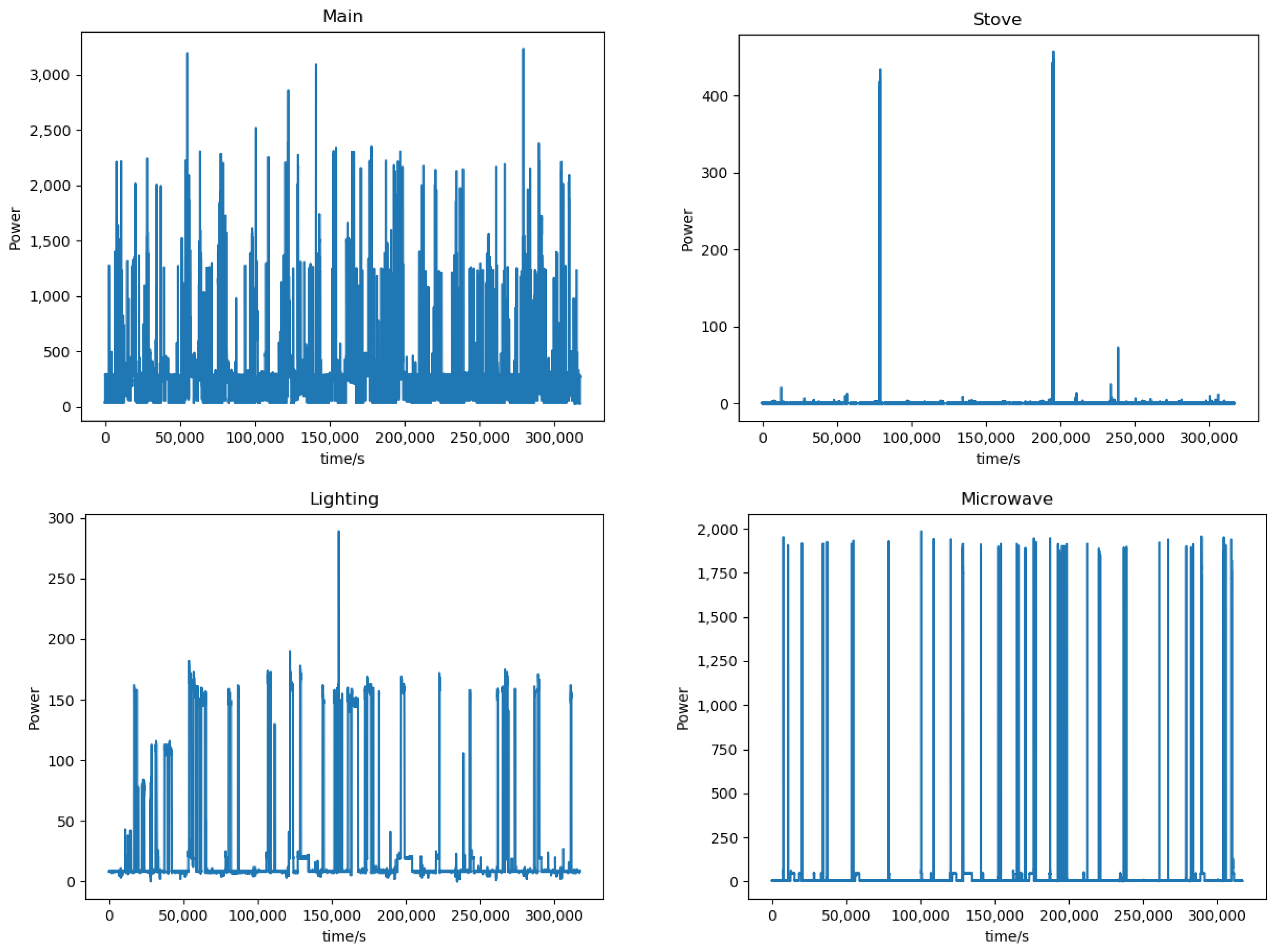
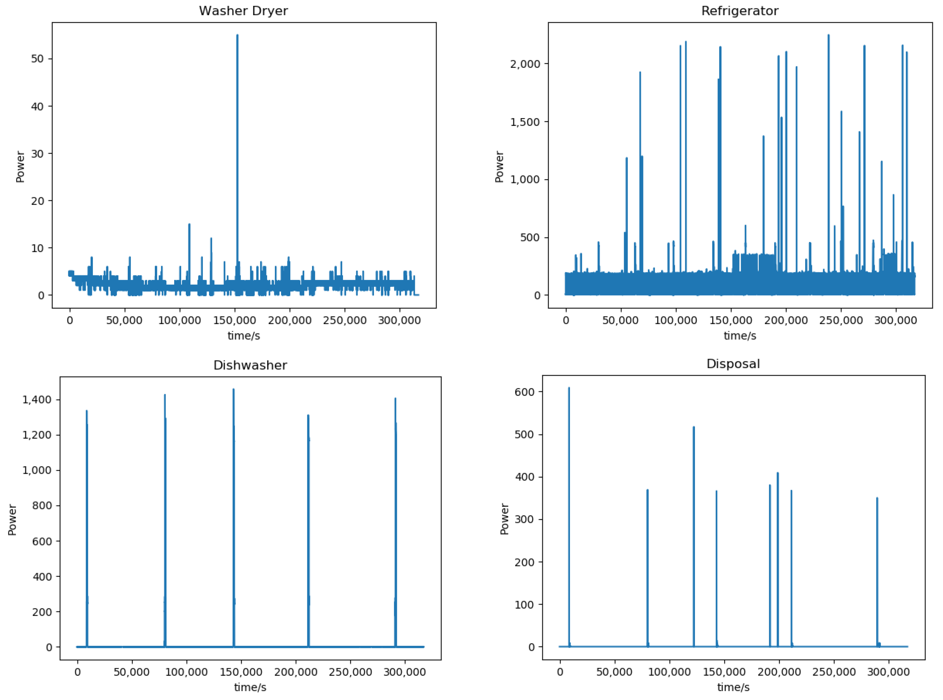
3.1. Data

The tests were conducted using real monitoring data from AMPds2 [14] and REDD house 2 [15]. The AMPds2 dataset collected the electricity usage of a Canadian family for two years, with a sampling frequency of one reading every minute. It monitored 24 appliances, but only 21 were kept, for they did not detect any data of the removed appliances for the entire measurement time. There were just a few missing data or errors in the dataset, and the algorithm was used to populate the missing data so that the whole dataset was contiguous. This facilitated the division of sequences in subsequent model training. In terms of electricity data, AMpds2 provided 11 measurements: voltage, current, frequency, displacement power factor, apparent power factor, real power, real energy, reactive power, reactive energy, apparent power, and apparent energy, which made it easy to select different features for improving model performance. Developed specifically for load disaggregation, the REDD dataset gathered real power consumption in some homes over several months, with a sampling frequency of approximately 3 s for every reading. In our experiments, we only used the data of house 2 in the REDD dataset, which included 10 types of equipment: lighting, refrigerator, dishwasher, washer-dryer, bathroom GFI, kitchen outlets, oven, microwave, electric heat, and stove.

3.2. Experimental Setup

Firstly, we segmented smart meter data into a sequence for AMPds2 datasets every 10 min and every 1 min for the REDD dataset, as discussed in Section 2.2. We chose the power measurements and current signals in AMPds2 and single power measurements in REDD for disaggregation. Then, we designed several templates for feature extraction.

Table 1. List of feature templates.

Templates 1	Templates 2	Templates 3	Meaning of the Template
$S_n$	$S_n$	$S_n$	current state
$S_{n-1}{S}_n$	$S_{n-1}{S}_n$	$S_{n-1}{S}_n$	current state and previous state
$S_{n-2}{S}_{n-1}{S}_n$	$S_{n-2}{S}_{n-1}{S}_n$	$S_{n-2}{S}_{n-1}{S}_n$	current state and previous two states
$S_{n-3}{}_{\dots }{S}_n$	/ 1	$S_{n-3}{}_{\dots }{S}_n$	current state and previous three states
$S_{n-4}{}_{\dots }{S}_n$	/	$S_{n-4}{}_{\dots }{S}_n$	current state and previous four states
$S_{n-5}{}_{\dots }{S}_n$	/	$S_{n-5}{}_{\dots }{S}_n$	current state and previous five states
$S_{n-6}{}_{\dots }{S}_n$	/	/	current state and previous six states
$S_{n-7}{}_{\dots }{S}_n$	/	/	current state and previous seven states
$S_{n-8}{}_{\dots }{S}_n$	/	/	current state and previous eight states

¹ This template does not have this feature.

shows the list of the feature templates used in our experiments. Among them, Templates 1 and 2 refer to the single power signature in REDD house 2 and AMPds2, respectively, while Templates 3 represent the double signatures: power and current in AMPds2.

Only extracting features over a continuous period of time was meaningful, which directly reflected the influence of previous states. If the time interval between two measurements is too large, for example 30 min, then it is not necessary to construct a transition function for these two measurements, because the state of an appliance half an hour ago has little effect on the current state. However, the timestamps in REDD house 2 was not continuous, so we found those intervals and just segmented data through those continuous data. Next, CRF++ [17] was used to build our model. CRF++ is an open-source CRF tool for continuous data annotation and segmentation, which is easy to use and customizable. We removed the features function for which the occurrences were less than three to further reduce the complexity of our model as claimed in Section 2.3. Additionally, a hyper-parameter C need to be selected in CRF++ to trade the balance between overfitting and underfitting. We found that the optimal value is 1.5 after cross-validation. All our work was carried out in Python 3 and C++. We also used 10-fold cross-validation to acquire the best error estimation.

3.3. Evaluation Metrics

In our paper, let $Acc$ be the accuracy, $T$ be the correct prediction, and $F$ be the incorrect prediction. Then, $Acc$ is defined as

$$Acc=\frac{T}{T+F}$$

(18)

This metric has normally been adopted by many researchers such as Stephen [13] and Kolter [15]. However, we do not think this indicator can properly reflect the performance of the model. Therefore, we adopted a new evaluation indicator: total load accuracy. Let $x_i,i=1,2,\dots ,N$ be the appliances monitored in the house, $l_j,j=1,2,\dots ,M$ be the observation sequences, and $TAcc$ be the total loads’ accuracy. We employed the following notation:

$$f(x_i,l_j,i,j)=\{\begin{array}{ll}1& \mathrm{if} \mathrm{the} \mathrm{predicted} \mathrm{state} \mathrm{of} i \mathrm{appliance} \mathrm{at} j\\ & \mathrm{is} \mathrm{the} \mathrm{same} \mathrm{as} \mathrm{the} \mathrm{real} \mathrm{state}\\ 0& \mathrm{otherwise}\end{array}$$

(19)

Then, the total loads’ accuracy $TAcc$ is defined as

$$TAcc=\frac{1}{M}{\displaystyle \sum }_{j=1}^M{\displaystyle \prod }_{i=1}^{N}f\left(x_i,l_j,i,j\right).$$

(20)

Each load has one state at any given time; the total load’s accuracy refers to the accuracy that all appliance states are assigned correctly at a given time. We combined this index for estimation because we believed that it could reflect the overall prediction ability of our model for the whole house. However, the accuracy results were generally lower than results in other papers, which only considered a single appliance’s on/off accuracy.

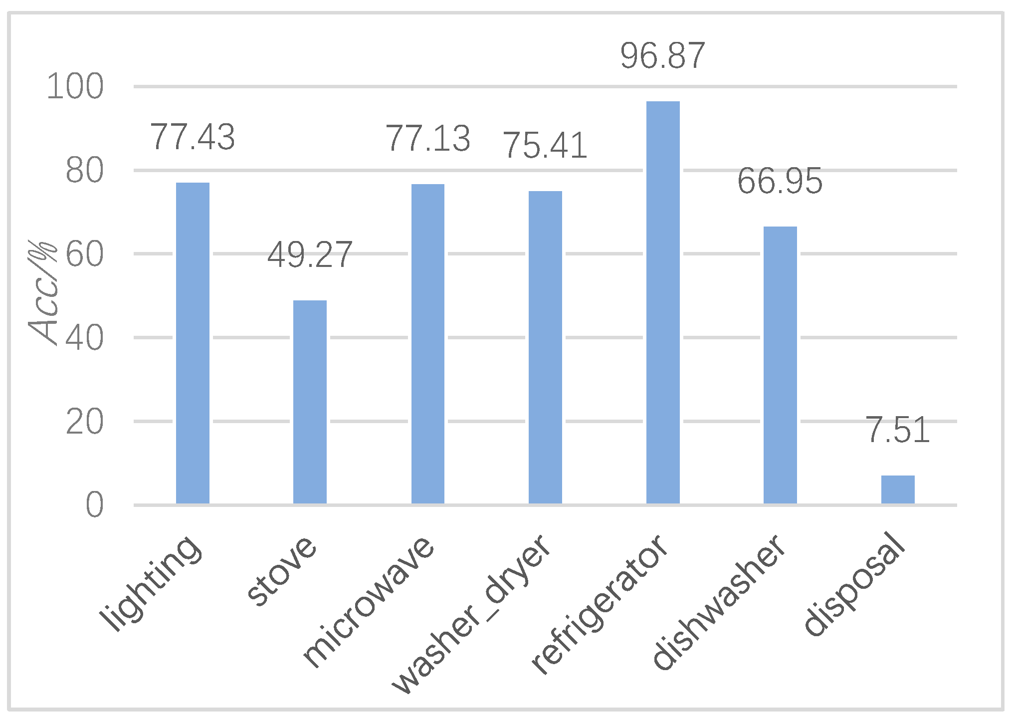
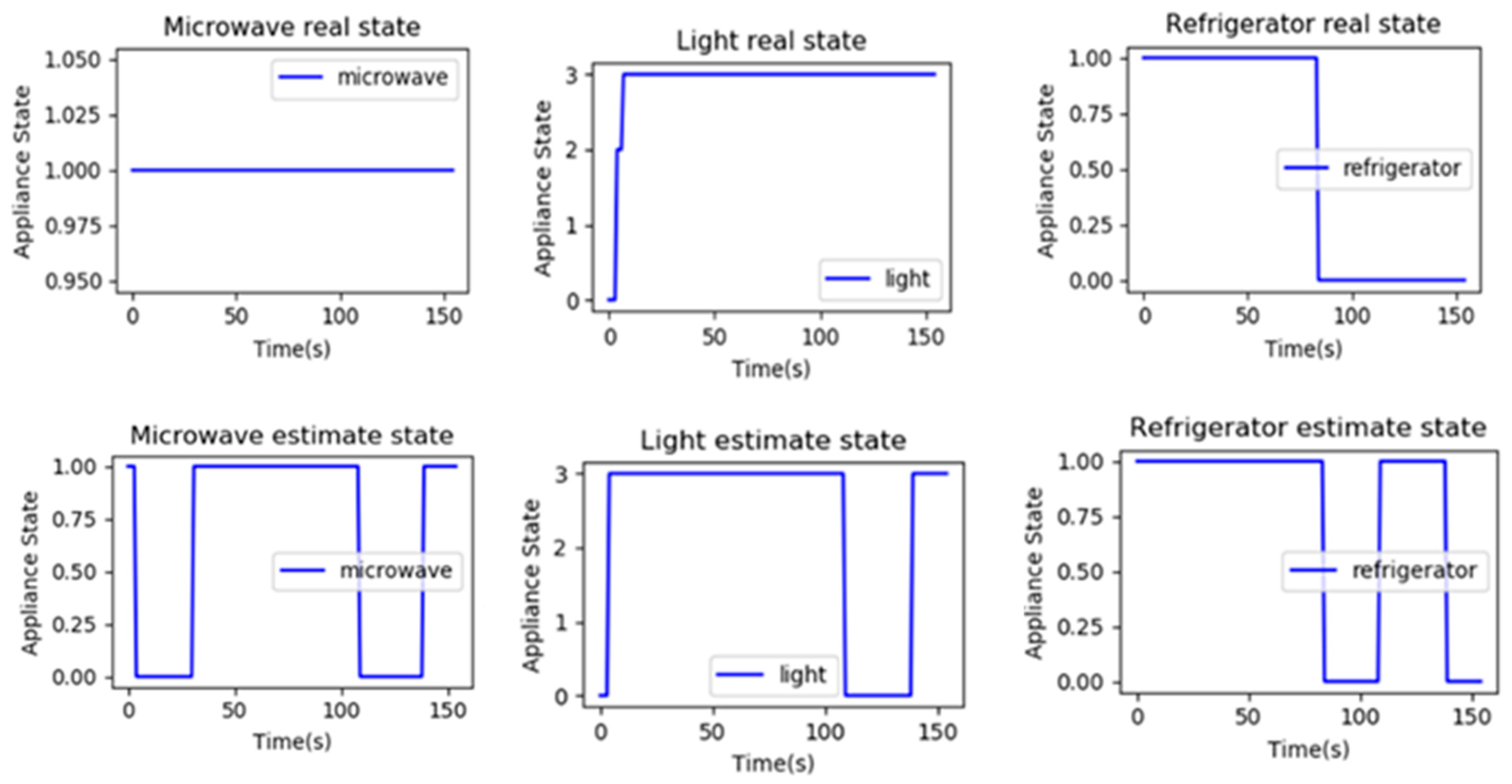
3.4. Experiment Results and Analysis

To better test the accuracy of our linear-chain CRF model, we chose seven appliances in REDD house 2: lighting, stove, microwave, washer-dryer, refrigerator, dishwasher, and disposal. Figure 7 illustrates the seven loads’ on-duration accuracy in REDD house 2. Obviously, the refrigerator showed the best score, while the disposal scores were very low. The low accuracy results were due to there being less disposal data working in the training sets. We also found that the power measures of the washer-dryer were mainly distributed from 0 to 10 all the time, which was purely low for a normal washer-dryer and similar to other appliances’ off state. Thus, our model mostly tagged the washer-dryer working when the measurements varied from 1 to 10, which made the accuracy results higher. We inferred that the washer-dryer in REDD house 2 did not work and the measurements were completely noisy.

We extracted some test sequences, as shown in Figure 8. It illustrates the real state changes of the electrical appliances which were working within a period of 150 s, as well as the inference results of our linear-chain CRF model according to the same data. It is clear that our model worked when different electrical appliances were used at the same time. Nevertheless, errors may have occurred when the power’s values of different working states of electrical appliances were similar. For example, during the period from 100 to 150 s, the total power decreased because the refrigerator stopped working. However, our model identified that the light and microwave stopped working while the refrigerator started working.

Figure 9 shows each test’s total loads’ accuracy in REDD house 2. Among them, 1 load refers to the refrigerator only; 2 loads mean the refrigerator and microwave; 3 loads stand for the kitchen outlets, microwave, and dishwasher; 4 loads indicate the lighting, microwave, washer-dryer, and refrigerator; 5 loads represent the refrigerator, lighting, dishwasher, microwave, and stove; 6 loads denote the lighting, stove, microwave, refrigerator, dishwasher, and disposal; 7 loads show the lighting, stove, microwave, washer-dryer, refrigerator, dishwasher, and disposal. We can see that the correct rate of accurate prediction of all electrical appliances at each moment was over 88% throughout the test time. This indicates that our model could correctly reflect the working state of all electrical appliances in the house tested at any time, not just for a single device.

As our linear-chain CRF model can combine more than one feature, we chose the current signals together with power measurements for parameter learning to test whether it promotes the performance of our model or not. Further, we hoped to estimate how well our model disaggregates loads in other datasets. We used five loads (including CDE, DWE, FRE, HPE, and WOE) in AMPds2 and verified the accuracy of a single power feature and double features. Figure 10 shows that using dual features can improve the efficiency to some extent. When it is challenging for the classifier to judge the state of the appliance only by the power value, the multiple features can provide an inferential basis by providing other state parameters. For example, our model performed much better in identifying the wall oven using double features, which was better than using a single feature by 32.49%.

In Stephen’s [13] paper, they used a sparsity HMM and obtained a perfect result. Thus, an experiment was conducted to assess the performance of the proposed linear-chain CRFs. We used REDD house 2 to test the performance for each model. Stephen divided their tests into three categories: Denoised, Noisy, and Modeled. Our tests belonged to the Noisy configuration, which neither removes the noise in the aggregate observation sequences nor tries to model the noise as a load [13]. Therefore, the Noisy configuration is the most realistic configuration for testing. We found that the use of different datasets and measurement metrics made it nearly impossible to compare different algorithms. Thus, the same datasets and measurement metrics have been used as recommended in Stephen’s paper. Firstly, we identified each load working state by quantizing its PMF. In Stephen’s [13] paper, they quantized both power and current observations. We just quantized power measurements, because it was enough to describe the working states for each appliance.

Table 2. Our state quantization results in AMPds2.

Appliance\Max power	0	1	2	3
B1E	1	6	623	\
BME	10	600	1571	\
DWE	8	300	848	\
EQE	20	34	52	\
FRE	50	300	581	\
HPE	500	2000	3701	\
UTE	0	10	41	65
WOE	0	2300	3200	3896
B2E	9	200	1000	\
CDE	7	1000	5614	\
FGE	8	400	1497	\
OUE	0	305	\ 1	\

¹ This type of appliance does not have this state.

and

Table 3. Stephen’s state quantization results.

Appliance\Max power	0	1	2	3
B1E	0	1	6	9999
BME	0	5	10	9999
DWE	0	4	8	9999
EQE	0	34	38	9999
FRE	0	100	107	9999
HPE	0	3	39	9999
UTE	0	10	41	9999
WOE	0	2	9999	\
B2E	0	5	9	9999
CDE	0	7	9999	\
FGE	0	3	8	9999
OUE	0	9999 1	\ 2	\

¹ The maximum power value set by Stephen. ² This type of appliance does not have this state.

show Stephen’s and our results for some appliance state quantization in the AMPds2 dataset. ‘\’ refers that the appliance does not have certain working state. In Stephen’s results, they classified the low-power operating state of the appliance in detail while grouping all high-power operating states into one state. Hence, the quantization results generated by Stephen are not reasonable. In contrast, we roughly clustered the appliances into a low-power operating state while dividing the high-power operating states in detail. That is more in line with the actual working state of the appliances.

Next, we compared some different appliance combinations in REDD house 2, and the results are shown in

Table 4. Accuracy comparison between the linear-chain CRF model and other algorithms.

Load\Acc (%)	Linear-Chain CRFs	Sparse HMM	SVM-rbf	SVM-Linear	SVM-Sigmoid
1 load	99.94	99.01	99.91	100	94.38
2 loads	99.27	99.00	98.39	96.32	81.82
3 loads	98.80	87.45	81.23	79.81	76.35
4 loads	96.04	98.52	92.40	90.31	88.41
5 loads	96.87	94.69	92.12	88.03	88.85
6 loads	97.40	95.28	93.22	85.83	88.84
7 loads	96.68	95.56	90.90	86.80	87.83

. The combinations are the same as in Figure 9. Our disaggregate results were slightly better than Stephen’s results, demonstrating that a basic linear-chain CRF model performs better, especially for the case that includes a kitchen outlet (three loads). Most common algorithms cannot deal with kitchen outlets because their power values change irregularly according to the appliances plugged into them. By extracting previous states, our model could improve accuracy to some extent. However, our model scored lower than sparse HMM when it came to four loads involving a washer-dryer. We found that the power value of the washer-dryer in REDD house 2 was excessively low. Thus, compared with HMM, which only extracted the last information, our model was more prone to obtaining errors.

In addition, the proposed method was compared with algorithms which were not based on the probabilistic graph model. We chose the SVM with three different kernels: radial basis function (rbf) kernel, linear kernel, and sigmoid kernel. There were several parameters that had to be determined cautiously to fit for the study, because a higher or lower figure can affect the results considerably and may lead to local maxima or overfitting. “C” is the penalty parameter of all three kernels, and “gamma” is the parameter of the rbf and sigmoid kernels. We employed a grid search to find the best parameters on a small scale of datasets. Then, we employed the best parameters to train the model on all of the training sets and then tested the performance on the test data. The best accuracy rate was obtained when C = 1.0 and gamma = 1.0. The accuracy results are shown in Table 4. It is clear that the rbf kernel was more suitable for identifying appliances in REDD house 2 compared with linear and sigmoid kernels. Moreover, the accuracy rates have a tendency to decrease when there are more appliances, while our model remained reliable. In fact, with the increase in the number of appliances, the total loads’ accuracy will decline as shown in Figure 9. However, by extracting a large number of state change characteristics of appliances, the recognition accuracy for most appliances can still be very high.

4. Conclusions

In this paper, we introduced a linear-chain CRF model for load disaggregation and demonstrated that this graphical model is feasible for a NILM task. We combined two features together: the power measurements and current signals. Feature templates were used for constructing feature functions, and the IIS algorithm was applied for parameter learning. Then, the Viterbi algorithm was utilized for decoding and estimated the accuracy results in AMPds2 and REDD house 2. Our accuracy results verified the feasibility and effectiveness of our model.

References

1. Hart, G.W. Nonintrusive appliance load monitoring. Proc. IEEE 1992, 80, 1870–1891. [Google Scholar] [CrossRef]
2. Lin, G.; Lee, S.; Hsu, J.Y.; Jih, W. Applying power meters for appliance recognition on the electric panel. In Proceedings of the 5th IEEE Conference on Industrial Electronics and Applications, Taichung, Taiwan, 15–17 June 2010; pp. 2254–2259. [Google Scholar]
3. Chui, K.T.; Lytras, M.D.; Visvizi, A. Energy Sustainability in Smart Cities: Artificial Intelligence, Smart Monitoring, and Optimization of Energy Consumption. Energies 2018, 11, 2869. [Google Scholar] [CrossRef]
4. Lai, Y.X.; Lai, C.F.; Huang, Y.M.; Chao, H.C. Multi-appliance recognition system with hybrid SVM/GMM classifier in ubiquitous smart home. Inf. Sci. 2013, 230, 39–55. [Google Scholar] [CrossRef]
5. Zia, T.; Bruckner, D.; Zaidi, A. A hidden Markov model-based procedure for identifying household electric loads. In Proceedings of the 37th Annual Conference of the IEEE Industrial Electronics Society, Melbourne, VIC, Australia, 7–10 November 2011; pp. 3218–3223. [Google Scholar]
6. Kong, W.; Dong, Z.Y.; Hill, D.J.; Ma, J.; Zhao, J.H.; Luo, F.J. A Hierarchical Hidden Markov Model Framework for Home Appliance Modeling. IEEE Trans. Smart Grid 2018, 9, 3079–3090. [Google Scholar] [CrossRef]
7. Kim, H.; Marwah, M.; Arlitt, M.; Lyon, G.; Han, J. Unsupervised Disaggregation of Low Frequency Power Measurements. In Proceedings of the 2011 SIAM International Conference on Data Mining, Mesa, AZ, USA, 28–30 April 2011; pp. 747–758. [Google Scholar]
8. Kolter, J.Z.; Jaakkola, T. Approximate Inference in Additive Factorial HMMs with Application to Energy Disaggregation. Neural Inf. Process. Syst. 2010, 22, 1472–1782. [Google Scholar]
9. Agyeman, K.A.; Han, S.; Han, S. Real-Time Recognition Non-Intrusive Electrical Appliance Monitoring Algorithm for a Residential Building Energy Management System. Energies 2015, 8, 9029–9048. [Google Scholar] [CrossRef] [Green Version]
10. Wallach, H.M. Conditional Random Fields: An Introduction. Tech. Rep. 2004, 267–272. [Google Scholar]
11. Lafferty, J.; McCallum, A.; Pereira, F. Conditional Random Fields: Probabilistic Models for Segmenting and Labeling Sequence Data. In Proceedings of the 18th International Conference on Machine Learning, Williams College, Williamstown, MA, USA, 28 June–1 July 2001; pp. 282–289. [Google Scholar]
12. Heracleous, P.; Angkititrakul, P.; Kitaoka, N.; Takeda, K. Unsupervised energy disaggregation using conditional random fields. In Proceedings of the IEEE PES Innovative Smart Grid Technologies, Europe, Istanbul, Turkey, 12–15 October 2014; pp. 1–5. [Google Scholar]
13. Makonin, S.; Popowich, F.; Bajic, I.V.; Gill, B.; Bartram, L. Exploiting HMM Sparsity to Perform Online Real-Time Nonintrusive Load Monitoring. IEEE Trans. Smart Grid 2016, 7, 2575–2585. [Google Scholar] [CrossRef]
14. Makonin, S.; Popowich, F.; Bartram, L.; Gill, B.; Bajic, I.V. AMPds: A public dataset for load disaggregation and eco-feedback research. In Proceedings of the 2013 IEEE Electrical Power & Energy Conference, Halifax, NS, Canada, 21–23 August 2013; pp. 1–6. [Google Scholar]
15. Kolter, J.Z.; Johnson, M.J. REDD: A Public Data Set for Energy Disaggregation Research. Available online: http://redd.csail.mit.edu/kolter-kddsust11.pdf (accessed on 10 May 2019).
16. Berger, A.L.; Pietra, V.J.D.; Pietra, S.A.D. A Maximum Entropy Approach to Natural Language Processing. Comput. Linguist. 1996, 22, 39–71. [Google Scholar]
17. CRF++. Available online: https://www.findbestopensource.com/product/crfpp (accessed on 21 April 2019).
Figure 1. Aggregated load data acquired from smart meters and disaggregating results produced from the model.
Energies 12 01797 g001aEnergies 12 01797 g001b
Figure 2. Main framework of our linear-chain CRF model for NILM.
Energies 12 01797 g002
Figure 3. Power probability density function of some appliances in AMPds2.
Energies 12 01797 g003aEnergies 12 01797 g003b
Figure 4. Power probability density function of some appliances in REDD house 2.
Energies 12 01797 g004aEnergies 12 01797 g004b
Figure 5. General graphical structure of a linear-chain CRF model.
Energies 12 01797 g005
Figure 6. Process of extracting features.
Energies 12 01797 g006
Figure 7. Seven loads’ on-duration accuracy in REDD house 2.
Energies 12 01797 g007
Figure 8. Comparison between appliances’ real and estimate states.
Energies 12 01797 g008
Figure 9. Each test total loads’ accuracy in REDD house 2.
Energies 12 01797 g009
Figure 10. (a) Radar charts with five loads (CDE, DWE, FRE, HPE, and WOE) accuracy in AMPds2. (b) Histogram charts with five loads accuracy. “Single” means that only power measurements were used, while “Double” means that power measurements and current signals were both included.
Energies 12 01797 g010