Magnetic Field during Wireless Charging in an Electric Vehicle According to Standard SAE J2954


Abstract
:1. Introduction
2. Magnetic Field Configuration According to SAE Recommended Practice J2954
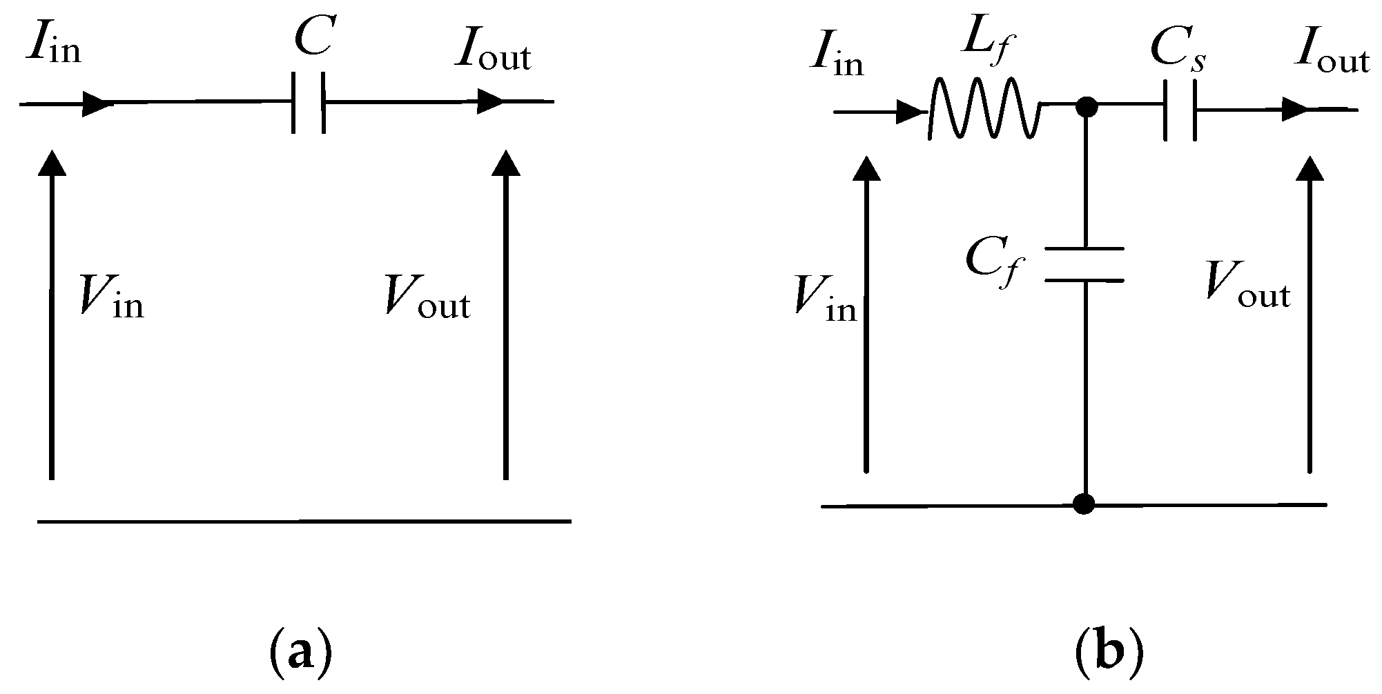
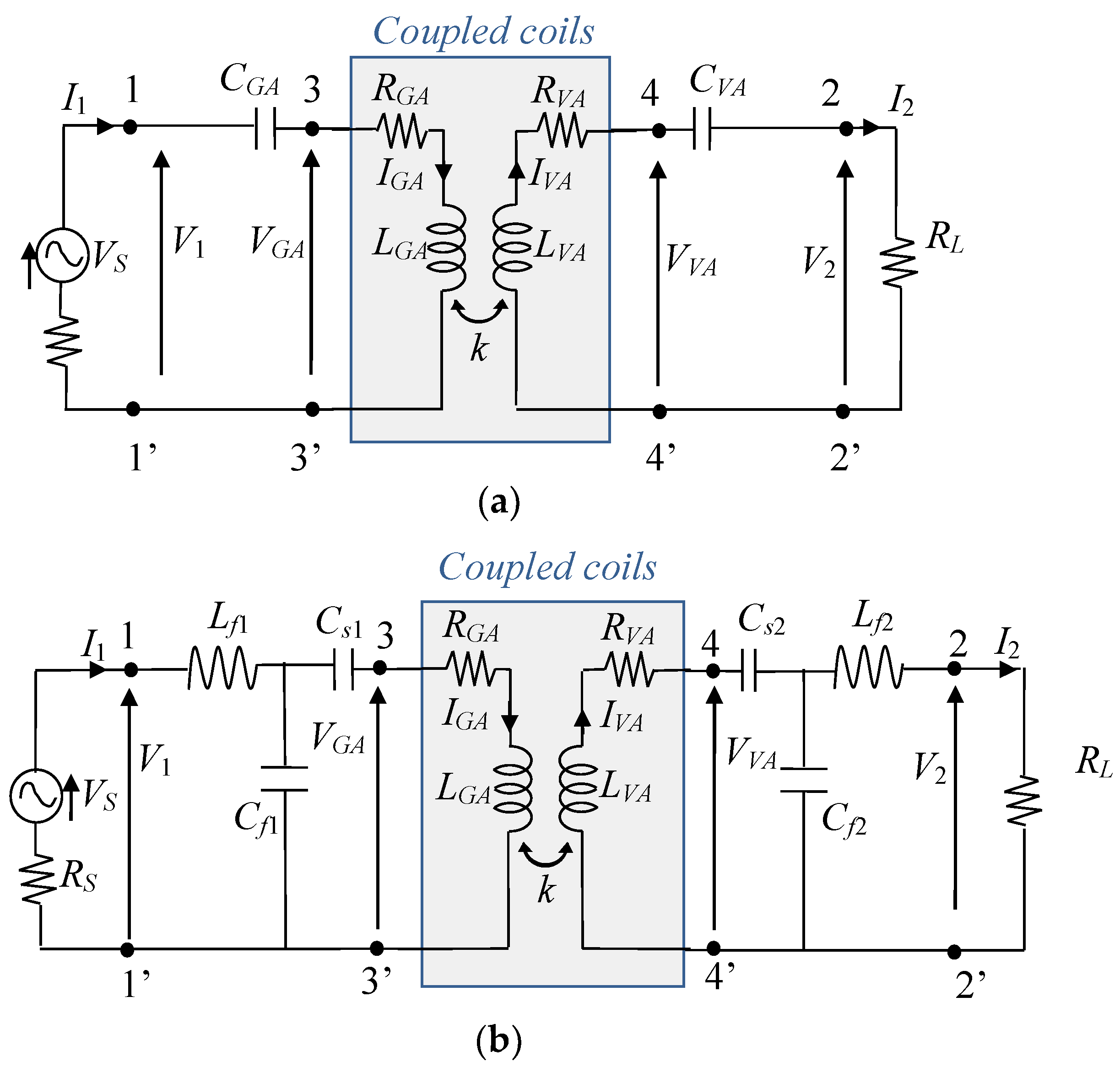
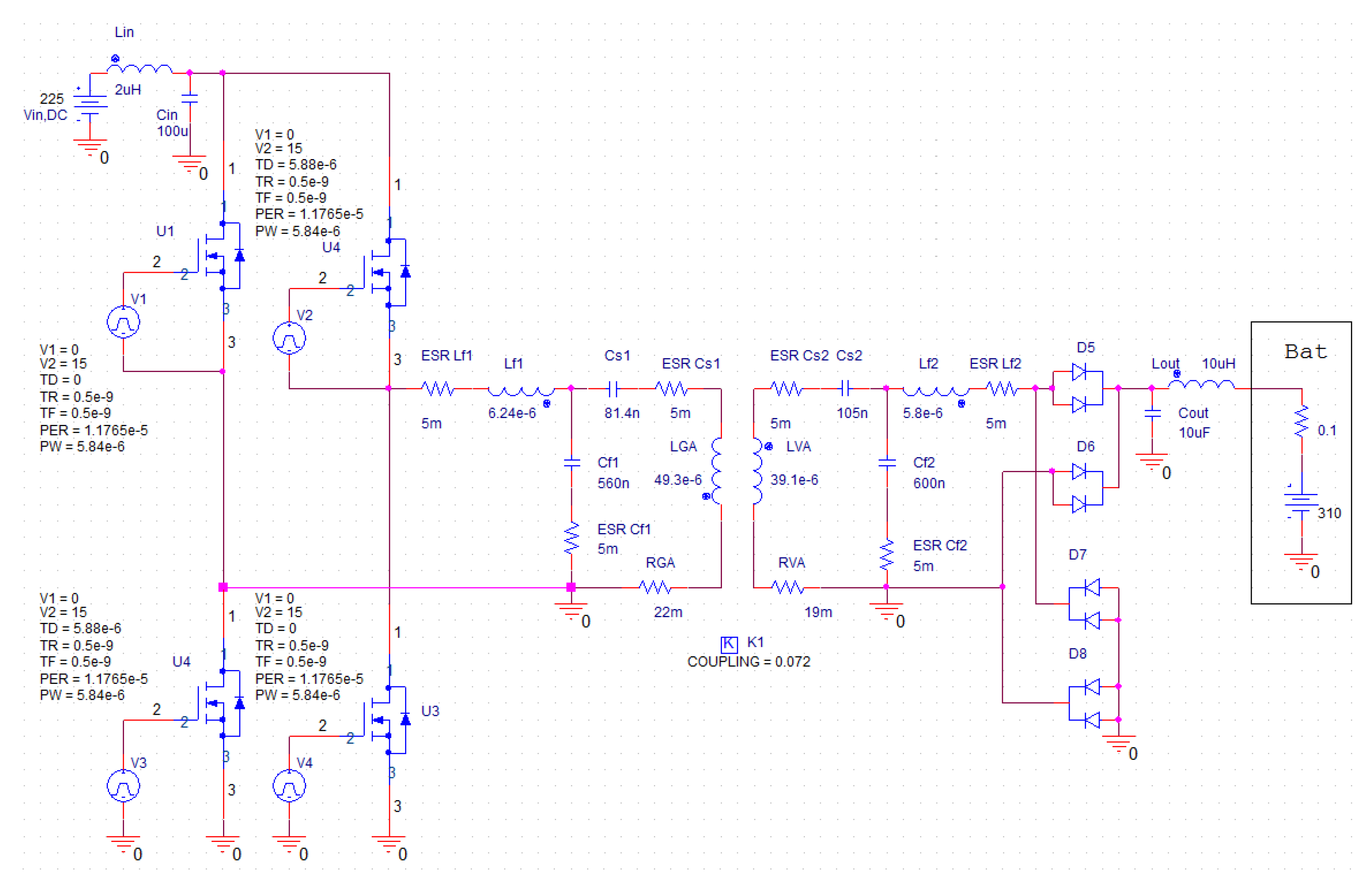
3. WPT Equivalent Circuit and Compensation Networks
4. Simulation Model
4.1. Field Equations
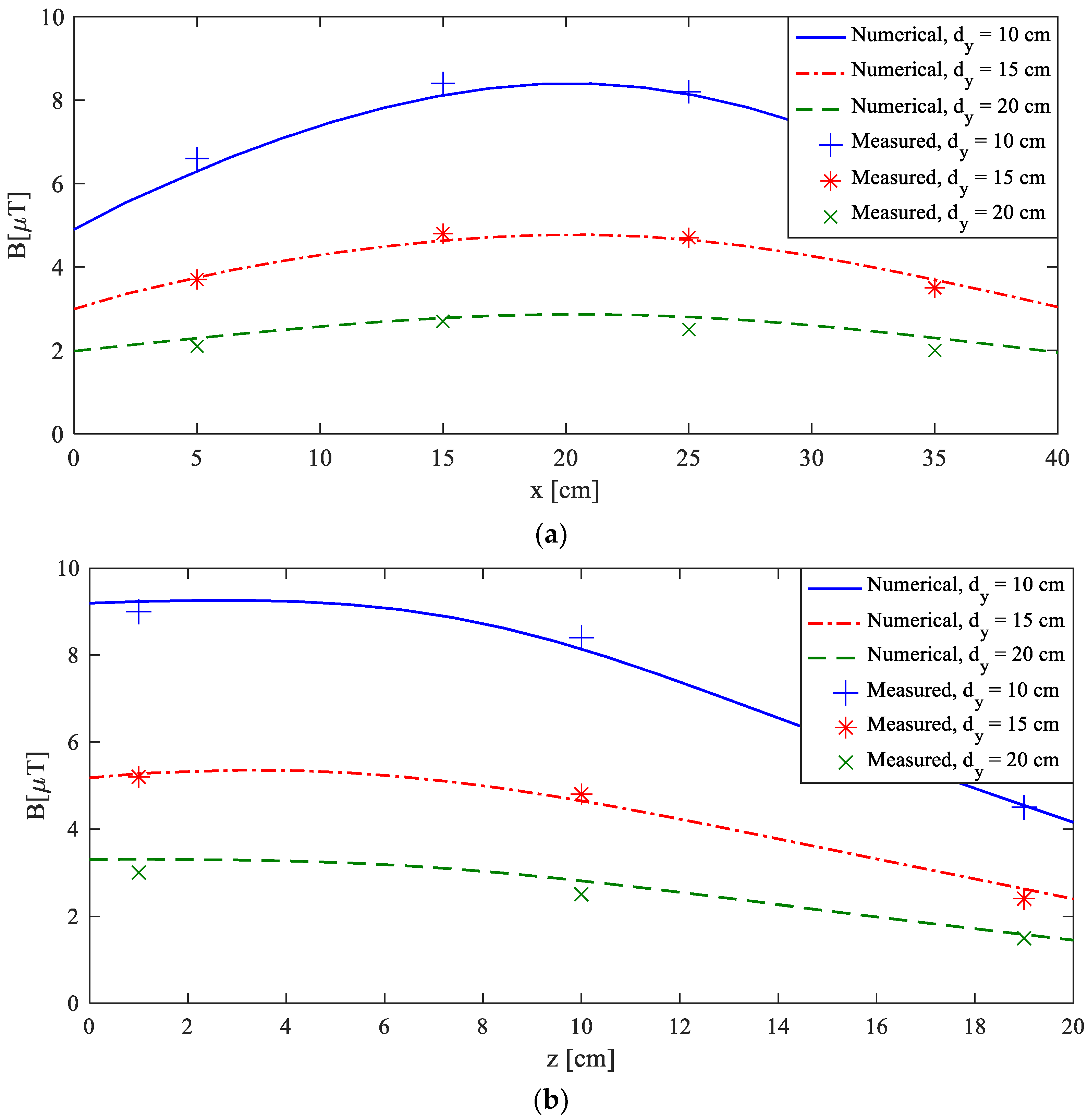
4.2. Circuit Parameters Extraction
5. Applications
5.1. WPT Systems
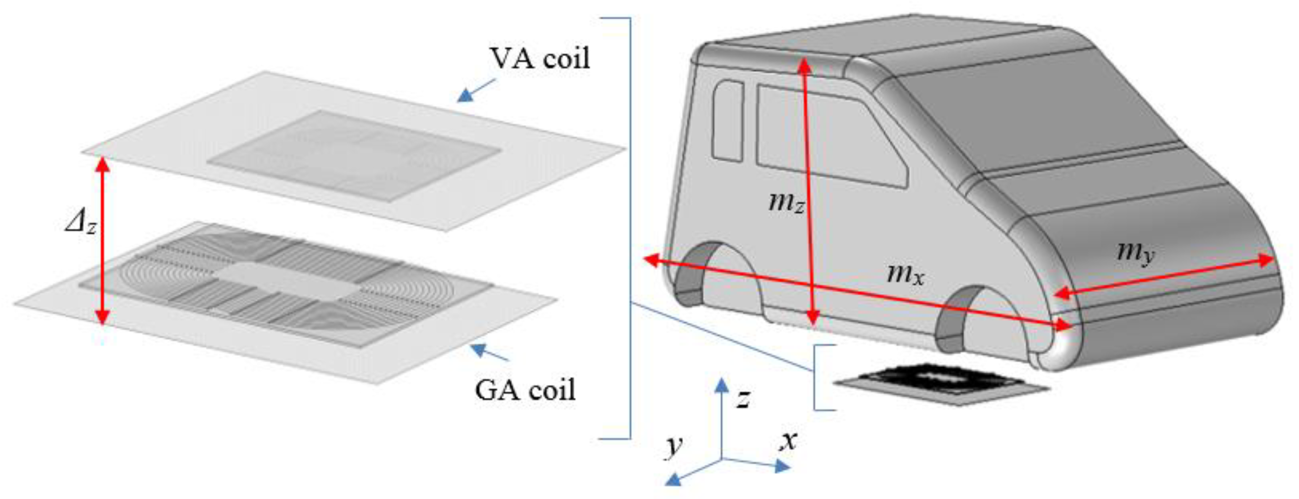
5.2. Car Body
5.3. System Performances
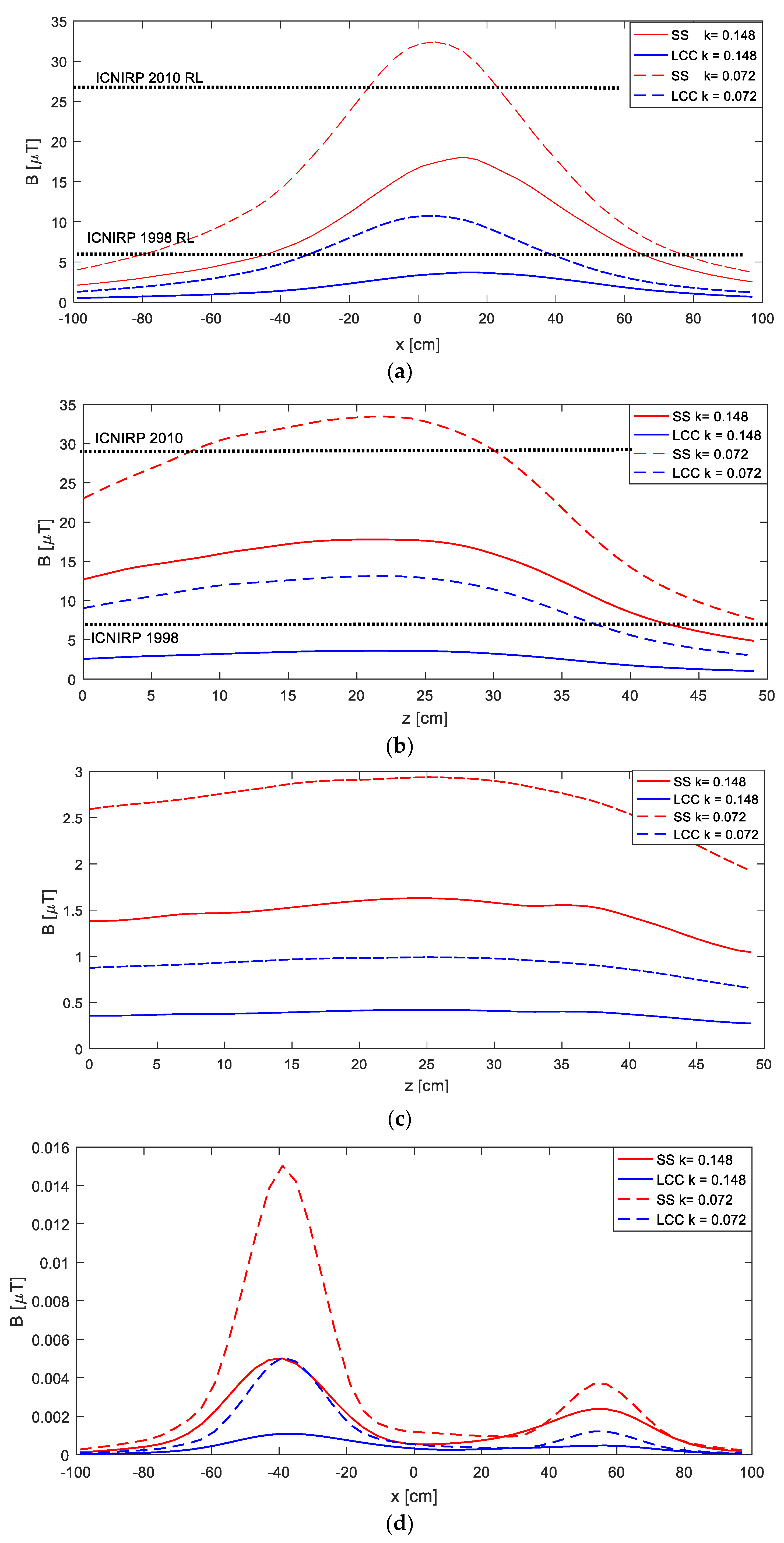
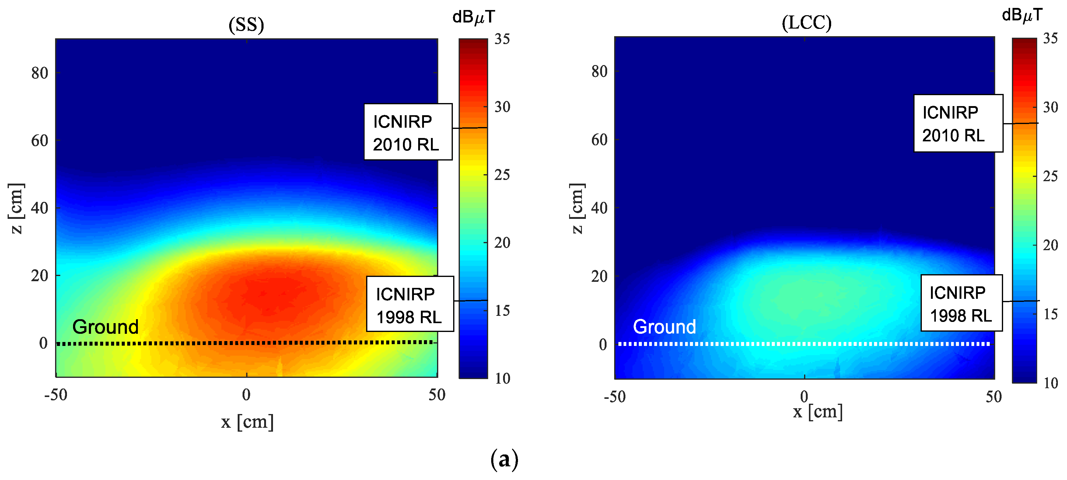
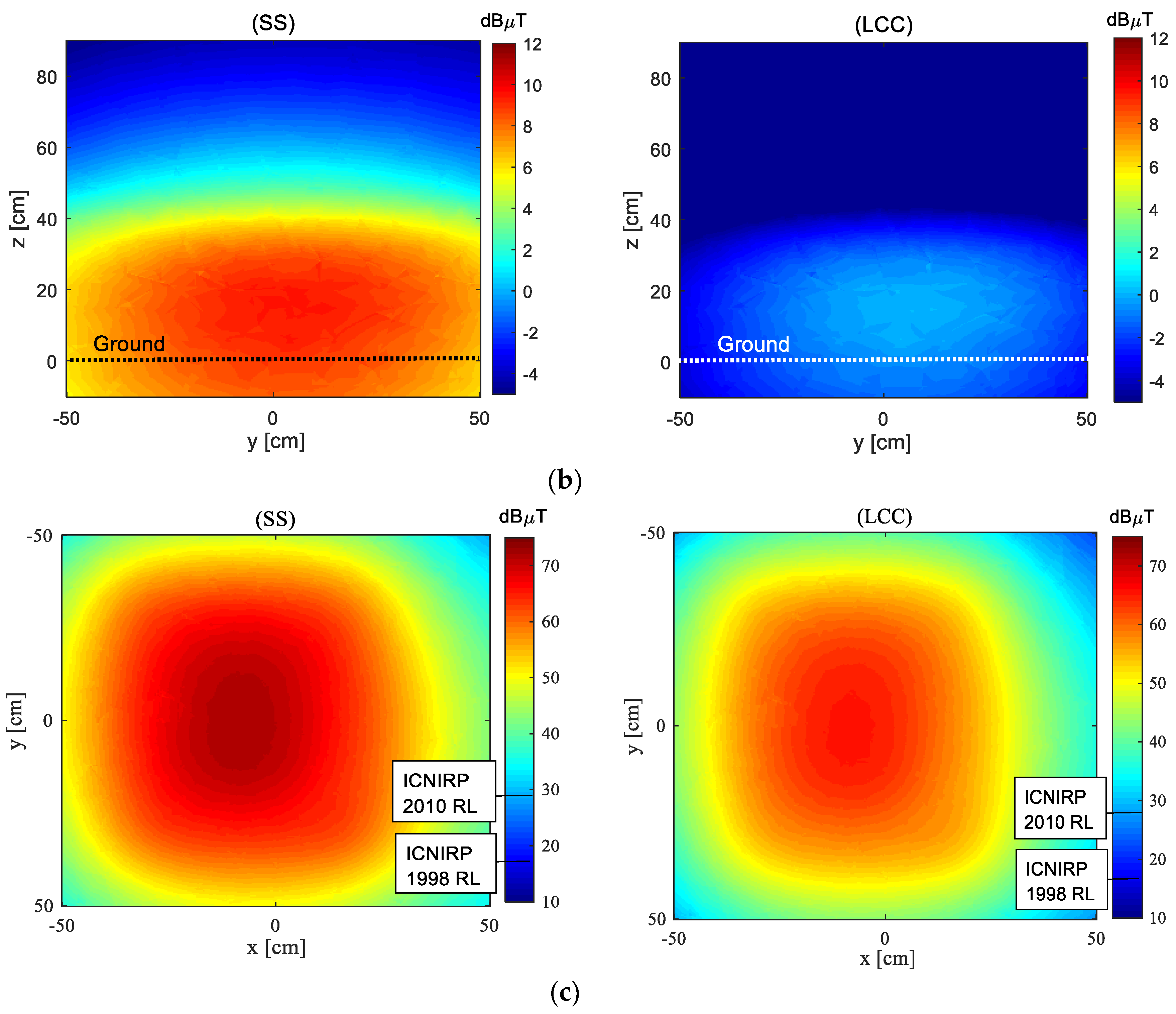
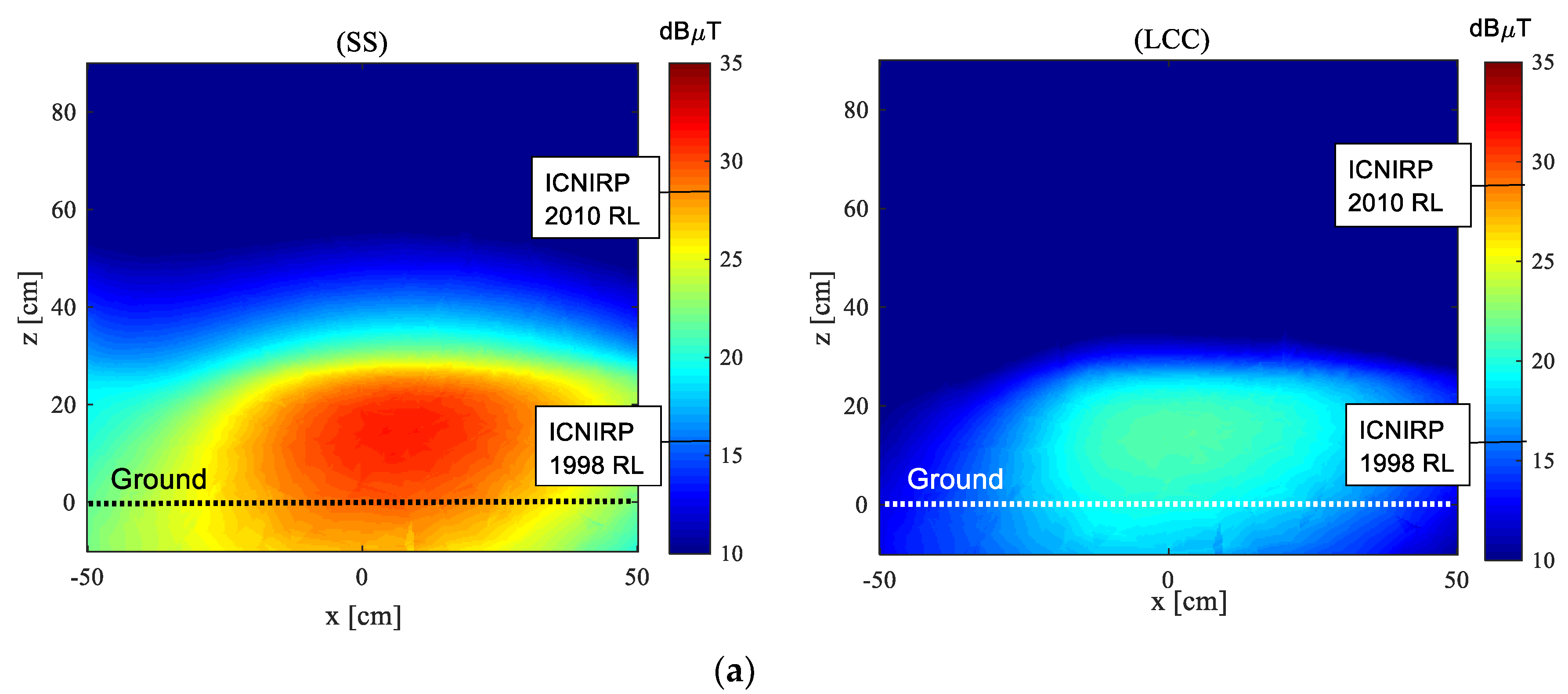
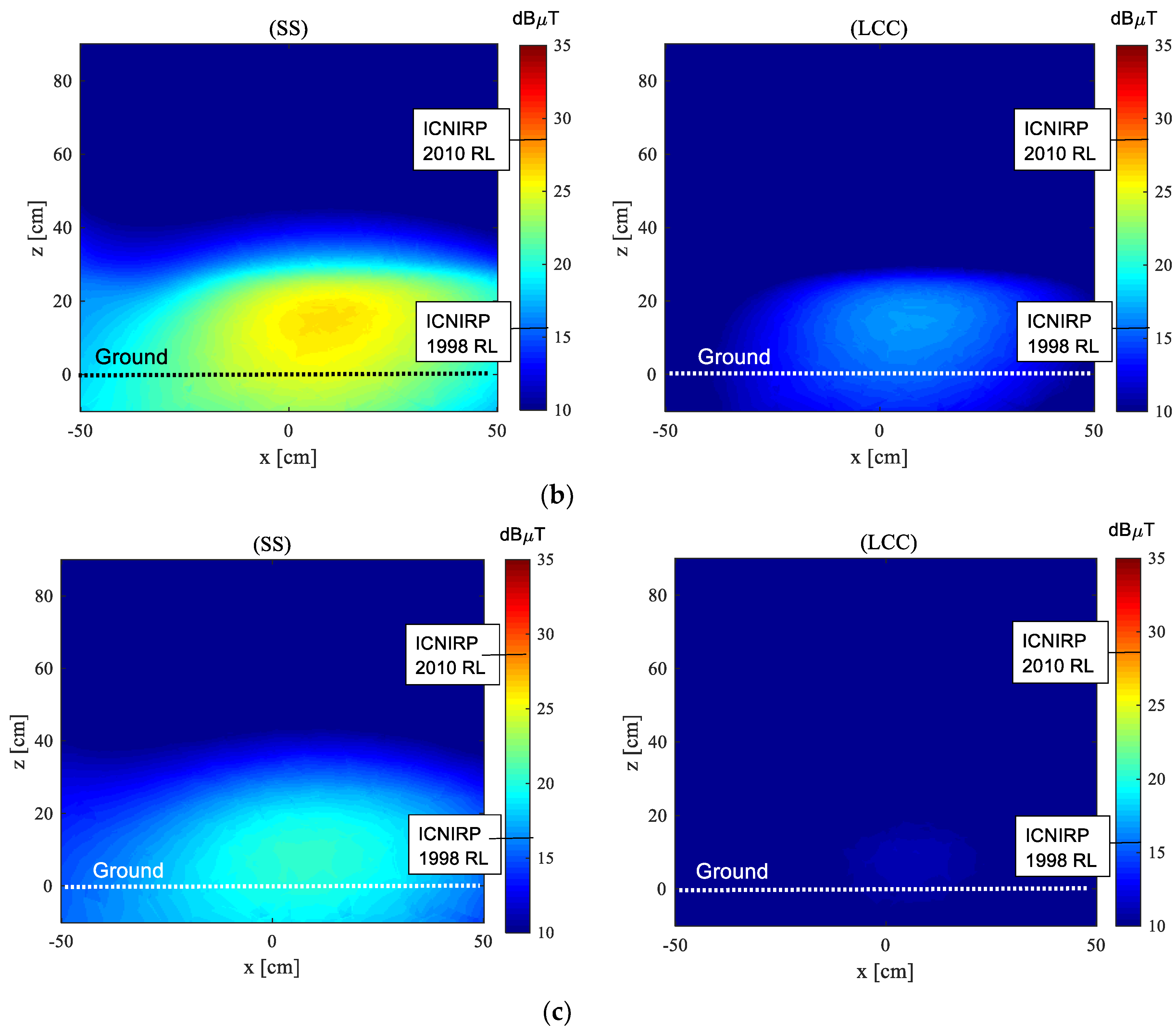
5.4. Magnetic Field Emission
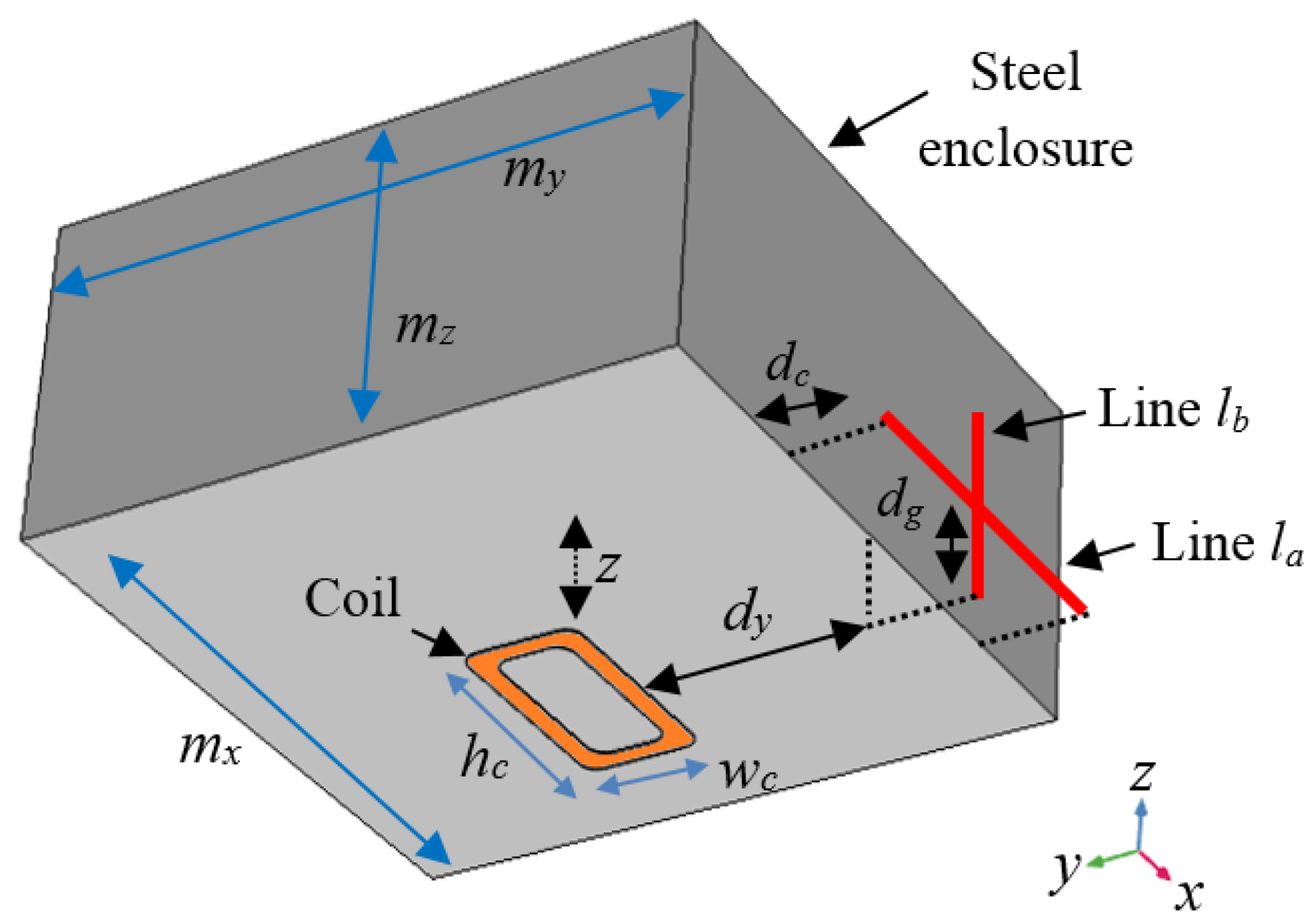
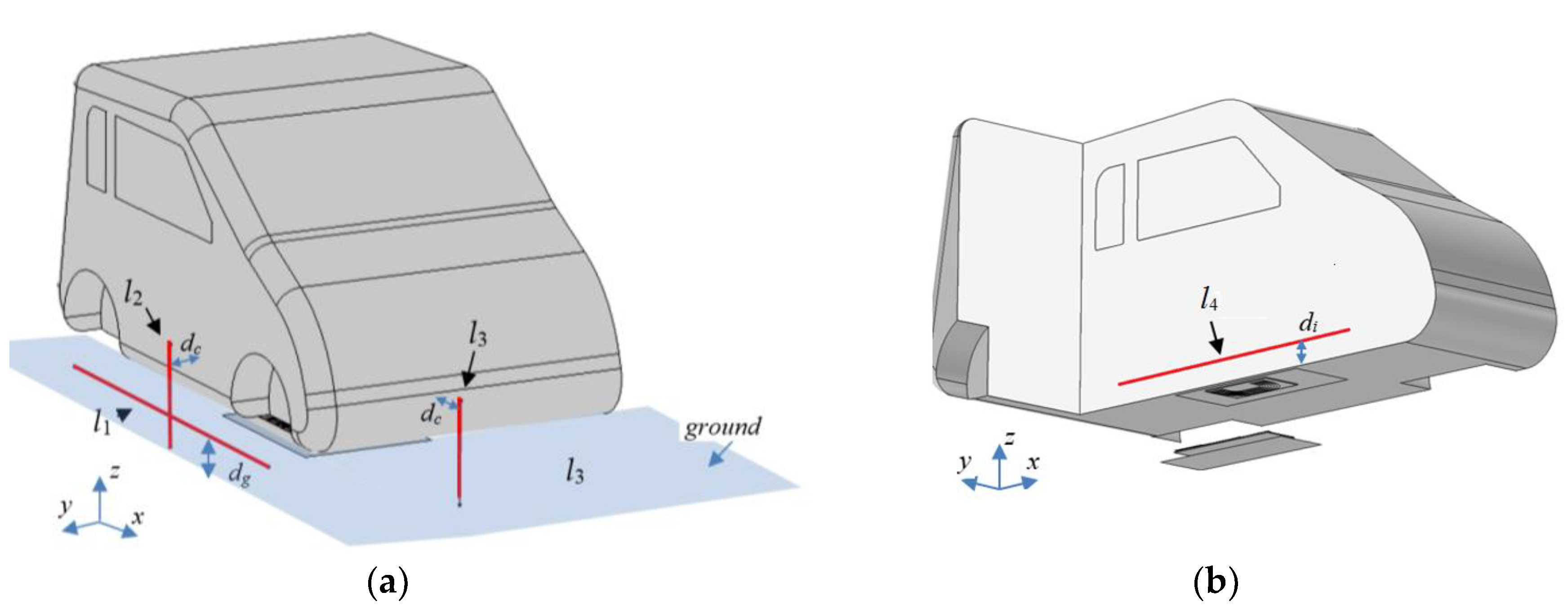
- Line 1 (l1): horizontal line parallel to the x axis on the side of the vehicle at a distance of dg = 150 mm from the ground and dc = 10 mm from the EV external side;
- Line 2 (l2): vertical line parallel to the z axis on the external side of the vehicle at a distance of dc = 10 mm from the EV external side;
- Line 3 (l3): vertical line parallel to the z axis on the front of the vehicle at a distance of dc = 10 mm from the EV external side;
- Line 4 (l4): horizontal line parallel to the x axis inside the cabin at a distance of di = 50 mm from the cabin floor.
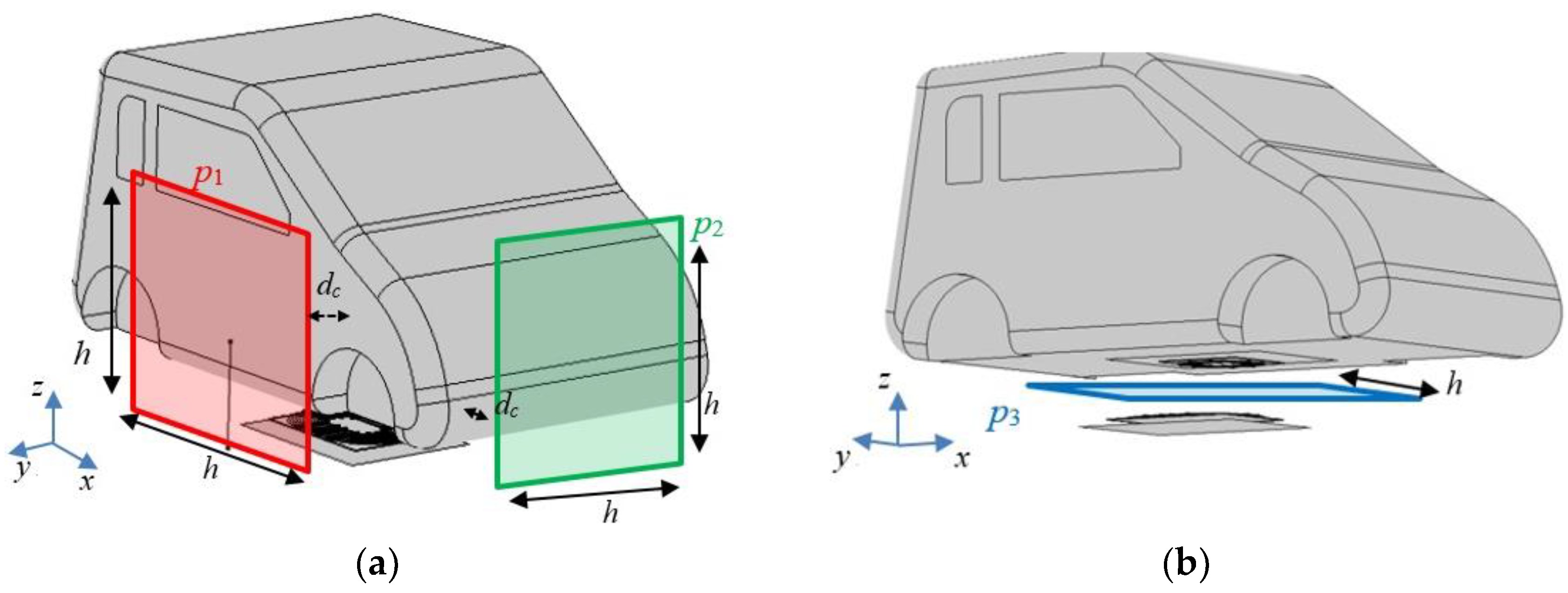
- p1: x-z plane beside the vehicle at a distance of dc = 10 mm from the body;
- p2: y-z plane on the front of the vehicle at a distance of dc = 10 mm from the body;
- p3: x-y plane between the coils under the vehicle at z = 125 mm from the ground.
- my = 1.6 m dy = 45 cm;
- my =1.7 m, dy = 50 cm;
- my =1.8 m, dy = 55 cm.
6. Conclusions
Author Contributions
Funding
Conflicts of Interest
References
- Covic, G.A.; Boys, J.T. Inductive power transfer. Proc. IEEE 2013, 101, 1276–1289. [Google Scholar] [CrossRef]
- Shinohara, N. Power without wires. IEEE Microw. Mag. 2011, 11, 64–73. [Google Scholar] [CrossRef]
- Wang, C.S.; Covic, G.A.; Stielau, O.H. Power Transfer Capability and Bifurcation Phenomena of Loosely Coupled Inductive Power Transfer Systems. Trans. Ind. Electron. 2004, 51, 148–157. [Google Scholar] [CrossRef]
- Ahmad, A.; Alam, M.S.; Chabaan, R.A. Comprehensive Review of Wireless Charging Technologies for Electric Vehicles. Trans. Transp. Electrif. 2018, 4, 38–63. [Google Scholar] [CrossRef]
- ISO/PAS 19363:2017. Electrically Propelled Road Vehicles—Connection to an External Electric Power Supply—Safety Requirements; ISO: Geneva, Switzerland, 2015. [Google Scholar] [CrossRef]
- IEC 61980-1:2015. Electric Vehicle Wireless Power Transfer (WPT) Systems—Part 1: General Requirements; International Electrotechnical Commission: Geneva, Switzerland, 2015. [Google Scholar]
- SAE Recommended Practice J2954 (rev. 201711). Wireless Power Transfer for Light-Duty Plug-In/ Electric Vehicles and Alignment Methodology; 27-11-2017; SAE International: Troy, MI, USA, 2017. [Google Scholar] [CrossRef]
- Schneider, J.; Carlson, R.; Sirota, J.; Sutton, R.; Taha, E.; Kesler, M.; Kamichi, K.; Teerlinck, I.; Abeta, H.; Minagawa, Y.; Yazaki, S. Validation of Wireless Power Transfer up to 11kW Based on SAE J2954 with Bench and Vehicle Testing; SAE International: Troy, MI, USA. [CrossRef]
- International Commission on Non-Ionizing Radiation Protection. Guidelines for limiting exposure to time-varying electric, magnetic, and electromagnetic fields (up to 300 GHz). Health Phys. 1998, 74, 494–522. [Google Scholar]
- International Commission on Non-Ionizing Radiation Protection. Guidelines for limiting exposure to time-varying electric and magnetic fields for low frequencies (1 Hz–100 kHz). Health Phys. 2010, 99, 818–836. [Google Scholar]
- Zhai, L.; Zhong, G.; Cao, Y.; Hu, G.; Li, X. Research on Magnetic Field Distribution and Characteristics of a 3.7 kW Wireless Charging System for Electric Vehicles under Offset. Energies 2019, 12, 392. [Google Scholar] [CrossRef]
- Feliziani, M.; Cruciani, S. Mitigation of the magnetic field generated by a wireless power transfer (WPT) system without reducing the WPT efficiency. In Proceedings of the International Symposium on Electromagnetic Compatibility, Brugge, Belgium, 2–6 September 2013; pp. 610–615. [Google Scholar]
- Campi, T.; Cruciani, S.; Feliziani, M. Magnetic Shielding of Wireless Power Transfer Systems. In Proceedings of the International Symposium on Electromagnetic Compatibility, Tokyo, Japan, 13–16 May 2014. [Google Scholar]
- Feliziani, M.; Cruciani, S.; Campi, T.; Maradei, F. Near field shielding of a wireless power transfer (WPT) current coil. Prog. Electromagn. Res. C 2017, 77, 39–48. [Google Scholar] [CrossRef]
- Campi, T.; Cruciani, S.; Feliziani, M. Numerical characterization of the magnetic field in electric vehicles equipped with a WPT system. Wirel. Power Transf. 2017, 4, 78–87. [Google Scholar] [CrossRef]
- Campi, T.; Cruciani, S.; Feliziani, M. Wireless power transfer (WPT) system for an electric vehicle (EV): How to shield the car from the magnetic field generated by two planar coils. Wirel. Power Transf. 2017, 5, 1–8. [Google Scholar] [CrossRef]
- Wang, Q.; Li, W.; Kang, J.; Wang, Y. Electromagnetic Safety Evaluation and Protection Methods for a Wireless Charging System in an Electric Vehicle. IEEE Trans. Electromagn. Compat. Early Access 2018, 1–13. [Google Scholar] [CrossRef]
- Moon, H.; Kim, S.; Park, H.H.; Ahn, S. Design of a resonant reactive shield with double coils and a phase shifter for wireless charging of electric vehicles. IEEE Trans. Magn. 2015, 51, 1–4. [Google Scholar] [CrossRef]
- Kim, S.; Park, H.; Kim, J. Design and Analysis of a Resonant Reactive Shield for a Wireless Power Electric Vehicle. IEEE Trans. Microw. Theory Tech. 2014, 62, 1057–1066. [Google Scholar] [CrossRef]
- Ding, P.; Bernard, L.; Pichon, L. Evaluation of Electromagnetic Field in Human Body Exposed to Wireless Inductive Charging System. IEEE Trans. Magn. 2014, 50, 1037–1040. [Google Scholar] [CrossRef]
- Laakso, I.; Hirata, A. Evaluation of the induced electric field and compliance procedure for a wireless power transfer system in an electrical vehicle. Phys. Med. Biol. 2013, 58, 7583. [Google Scholar] [CrossRef] [PubMed]
- Zhang, K.H.; Du, L.N.; Zhu, Z.B.; Song, B.W.; Xu, D.M. A Normalization Method of Delimiting the Electromagnetic Hazard Region of a Wireless Power Transfer System. IEEE Trans. Electromagn. Compat. 2018, 60, 829–839. [Google Scholar] [CrossRef]
- Kim, S.; Covic, G.A.; Boys, J.T. Comparison of Tripolar and Circular Pads for IPT Charging Systems. IEEE Trans. Power Electron. 2018, 33, 6093–6103. [Google Scholar] [CrossRef]
- De Santis, V.; Campi, T.; Cruciani, S.; Laakso, I.; Feliziani, M. Assessment of the Induced Electric Fields in a Carbon-Fiber Electrical Vehicle Equipped with a Wireless Power Transfer System. Energies 2018, 11, 684. [Google Scholar] [CrossRef]
- Yan, Z.; Zhang, Y.; Song, B.; Zhang, K.; Kan, T.; Mi, C. An LCC-P Compensated Wireless Power Transfer System with a Constant Current Output and Reduced Receiver Size. Energies 2019, 12, 172. [Google Scholar] [CrossRef]
- Ann, S.; Lee, W.Y.; Choe, G.Y.; Lee, B.K. Integrated Control Strategy for Inductive Power Transfer Systems with Primary-Side LCC Network for Load-Average Efficiency Improvement. Energies 2019, 12, 312. [Google Scholar] [CrossRef]
- Li, S.; Li, W.; Deng, J.; Nguyen, T.D.; Mi, C.C. A double-sided LCC compensation network and its tuning method for wireless power transfer. IEEE Trans. Veh. Technol. 2015, 64, 2261–2273. [Google Scholar] [CrossRef]
- Feliziani, M.; Campi, T.; Cruciani, S.; Maradei, F.; Grasselli, U.; Macellari, M.; Schirone, M. Robust LCC compensation in wireless power transfer with variable coupling factor due to coil misalignment. In Proceedings of the IEEE 15th International Conference on Environment and Electrical Engineering (EEEIC), Rome, Italy, 10–13 June 2015; pp. 1181–1186. [Google Scholar] [CrossRef]
- Campi, T.; Cruciani, S.; Maradei, F.; Feliziani, M. Near Field reduction in a Wireless Power Transfer System using LCC compensation. IEEE Trans. Electromagn. Compat. 2017, 59, 686–694. [Google Scholar] [CrossRef]
- Feliziani, M.; Maradei, F. Edge element analysis of complex configurations in presence of thin shields. IEEE Trans. Magn. 1997, 33, 1548–1551. [Google Scholar] [CrossRef]
- Feliziani, M.; Maradei, F. Fast computation of quasi-static magnetic fields around nonperfectly conductive shields. IEEE Trans. Magn. 1998, 34, 2795–2798. [Google Scholar] [CrossRef]
- Buccella, C.; Feliziani, M.; Fuina, V. ELF magnetic field mitigation by active shielding. In Proceedings of the IEEE International Symposium on Industrial Electronics ISIE-02, L’Aquila, Italy, 8–11 July 2002. [Google Scholar] [CrossRef]
- Feliziani, M.; Cruciani, S. FDTD modeling of impedance boundary conditions by equivalent LTI circuits. IEEE Trans. Microw. Theory Tech. 2012, 60, 3656–3666. [Google Scholar] [CrossRef]
- Feliziani, M.; Maradei, F.; Tribellini, G. Field analysis of penetrable conductive shields by the finite-difference time-domain method with impedance network boundary conditions (INBCs). IEEE Trans. Electromag. Compat. 1999, 41, 307–319. [Google Scholar] [CrossRef]
- Feliziani, M. Subcell FDTD modeling of field penetration through lossy shields. IEEE Trans. Electromag. Compat. 2012, 54, 299–307. [Google Scholar] [CrossRef]
- Feliziani, M.; Cruciani, S.; Campi, T.; Maradei, F. Artificial Material Single Layer to Model the Field Penetration Through Thin Shields in Finite-Elements Analysis. IEEE Trans. Microw. Theory Techn. 2018, 66, 56–63. [Google Scholar] [CrossRef]
- Cruciani, S.; Campi, T.; Maradei, F.; Feliziani, M. Conductive Layer Modeling by Improved Second-Order Artificial Material Single-Layer Method. Trans. Antennas Propag. 2018, 66, 5646–5650. [Google Scholar] [CrossRef]
- Cruciani, S.; Campi, T.; Maradei, F.; Feliziani, M. Artificial material single-layer method applied to model the electromagnetic field propagation through anisotropic shields. IEEE Trans. Microw. Theory Tech. 2018, 66, 3756–3763. [Google Scholar] [CrossRef]
- Spadacini, G.; Grassi, F.; Pignari, S.A. Modelling and simulation of conducted emissions in the powertrain of electric vehicles. Prog. Electromagn. Res. B 2016, 69, 1–15. [Google Scholar] [CrossRef]
- European Council Recommendation of 12 July 1999 on the Limitation of Exposure of the General Public to Electromagnetic Fields (0 Hz to 300 GHz) (1999/519 CE). Available online: http://data.europa.eu/eli/reco/1999/519/oj (accessed on 18 April 2019).


| Outer Dimension | GA | VA | ||||
|---|---|---|---|---|---|---|
| Length (mm) | Width (mm) | Thickness (mm) | Length (mm) | Width (mm) | Thickness (mm) | |
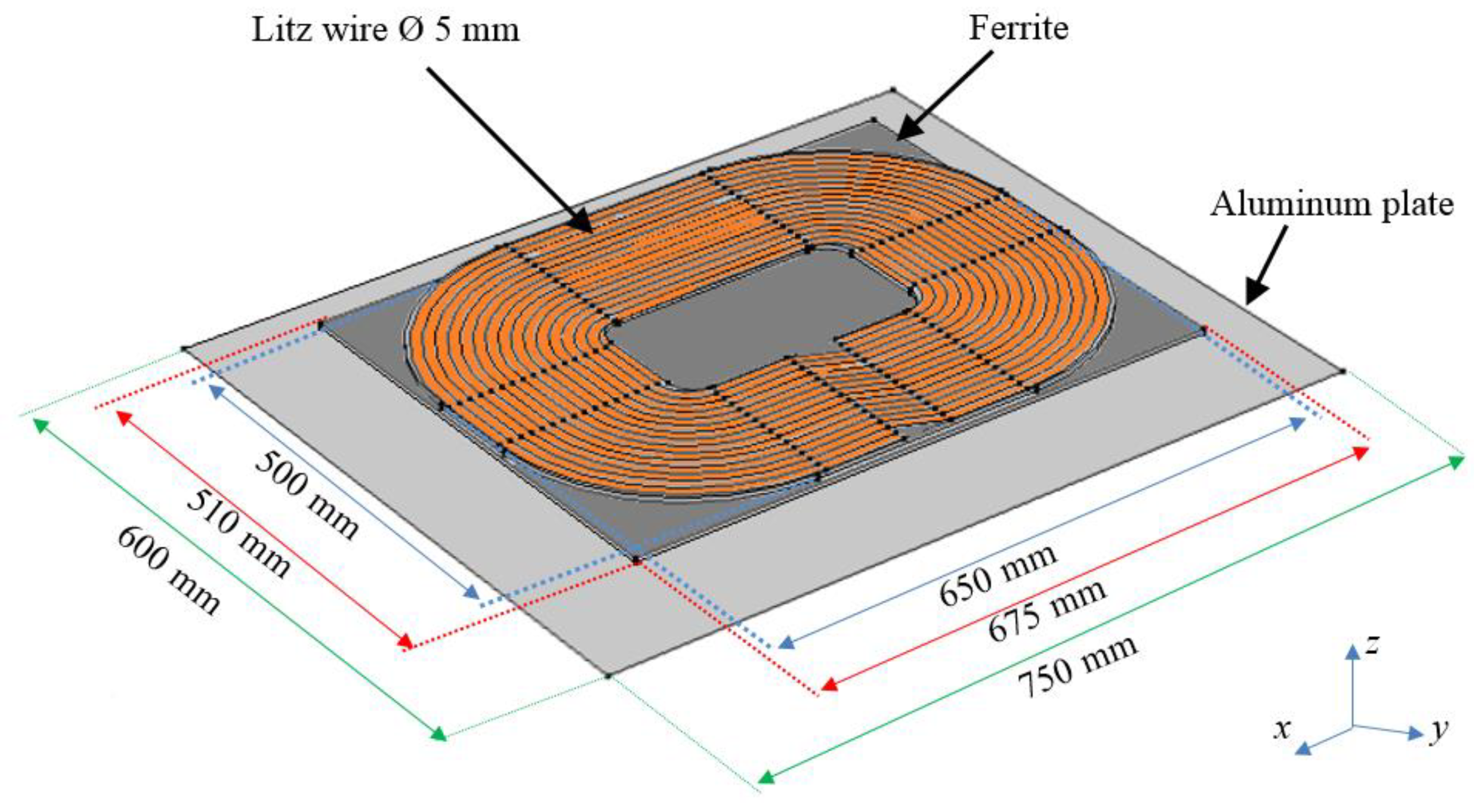
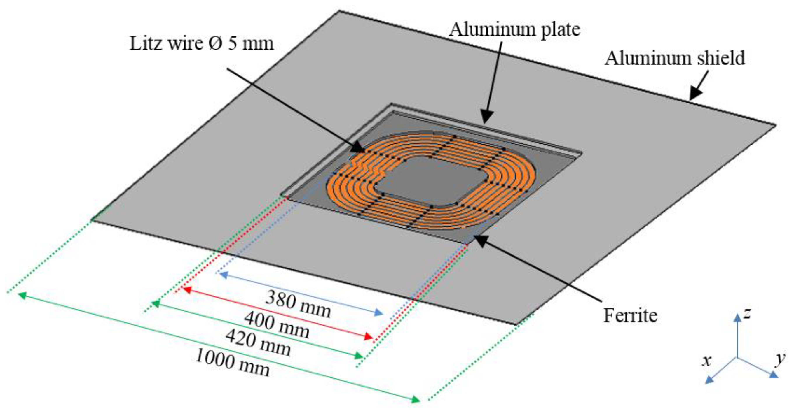
| Winding | 650 | 500 | 5 | 380 | 380 | 5 |
| Ferrite shield | 675 | 510 | 5 | 400 | 400 | 5 |
| Aluminum plate | 750 | 600 | 2 | 420 | 420 | 3 |
| Aluminum shield | / | / | / | 1000 | 1000 | 2 |
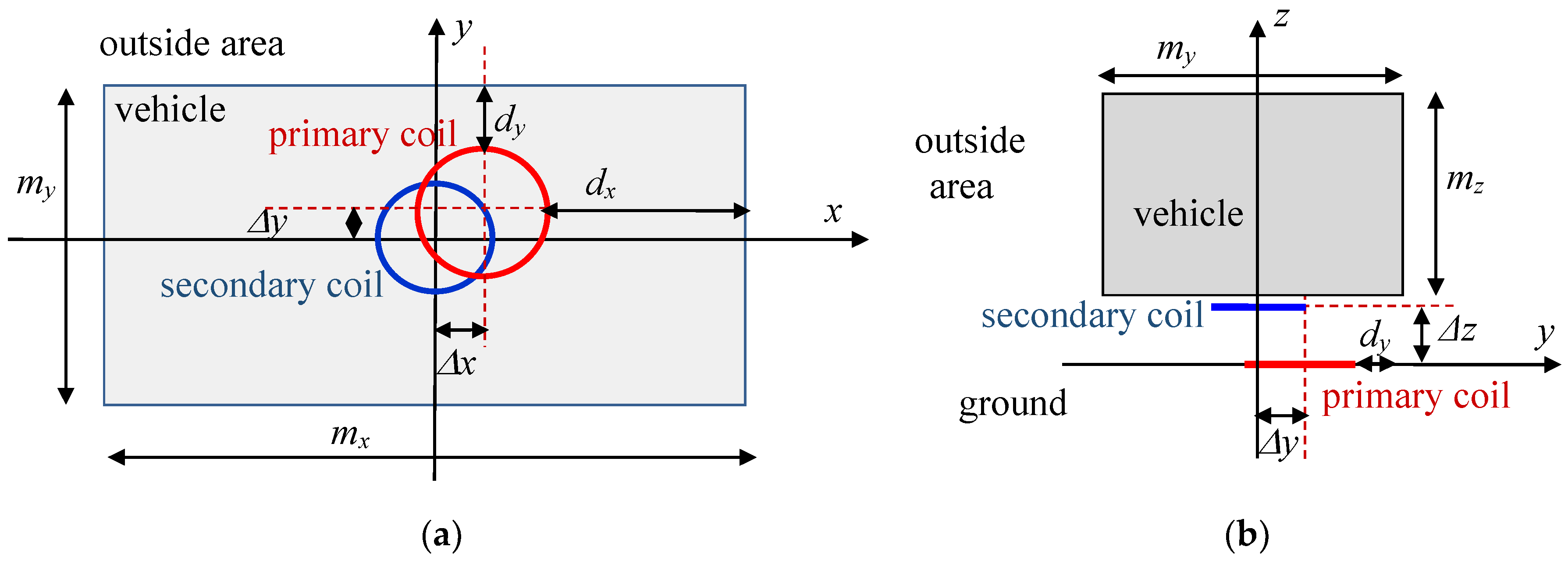
| Δz (mm) | Δx (mm) | Δy (mm) | LGA (μH) | LVA (μH) | M (μH) | k |
|---|---|---|---|---|---|---|
| 200 | 0 | 0 | 50.4 | 39.9 | 6.5 | 0.148 |
| 200 | 75 | 0 | 50.6 | 39.9 | 5.75 | 0.131 |
| 200 | 75 | 100 | 50.6 | 40.0 | 4.75 | 0.110 |
| 250 | 0 | 0 | 49.2 | 39.1 | 4.5 | 0.102 |
| 250 | 75 | 0 | 49.3 | 39.0 | 3.8 | 0.087 |
| 250 | 75 | 100 | 49.3 | 39.0 | 3.2 | 0.072 |
| Compensation | CVA (nF) | Cs1 (nF) | Cf1 (nF) | Lf1 (μH) | CGA (nF) | Cs2 (nF) | Cf2 (nF) | Lf2 (μH) |
|---|---|---|---|---|---|---|---|---|
| SS | 71.4 | \ | \ | \ | 89.9 | \ | \ | \ |
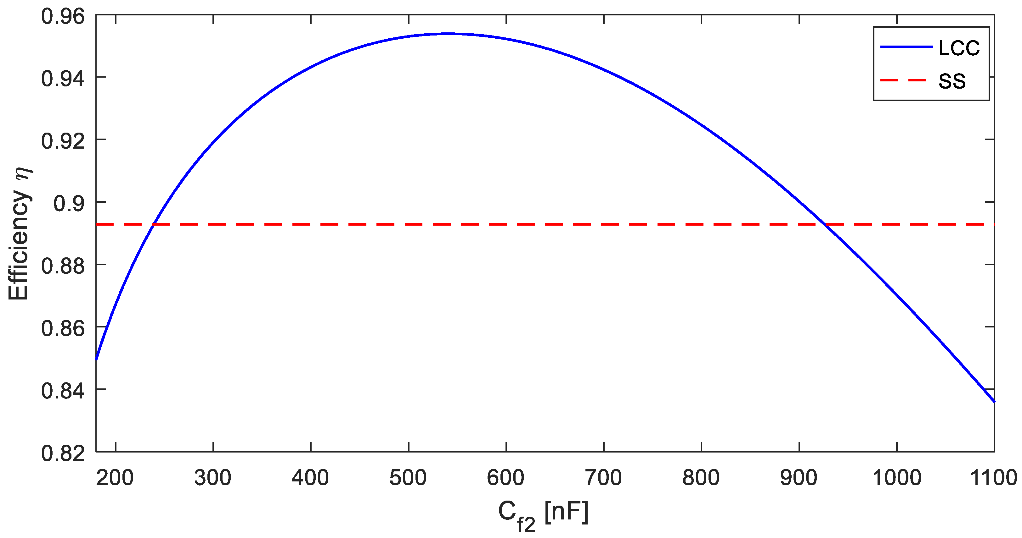
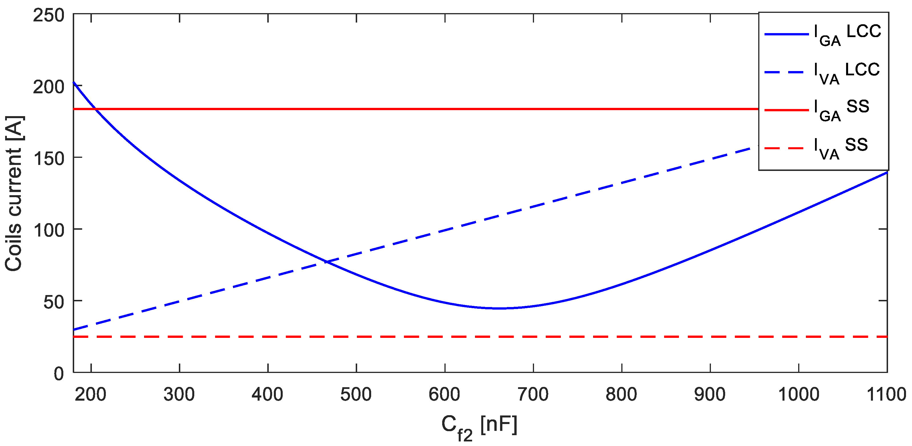
| LCC | \ | 81.4 | 560 | 6.24 | \ | 105 | 600 | 5.5 |
| k | SS | LCC | ||||||
|---|---|---|---|---|---|---|---|---|
| IGA (A) | IVA (A) | η | α (deg) | IGA (A) | IVA (A) | η | α (deg) | |
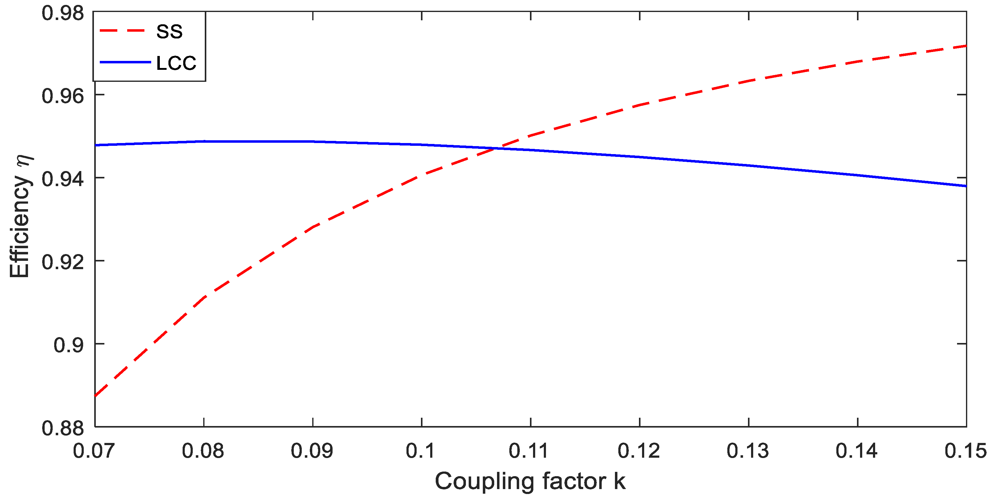
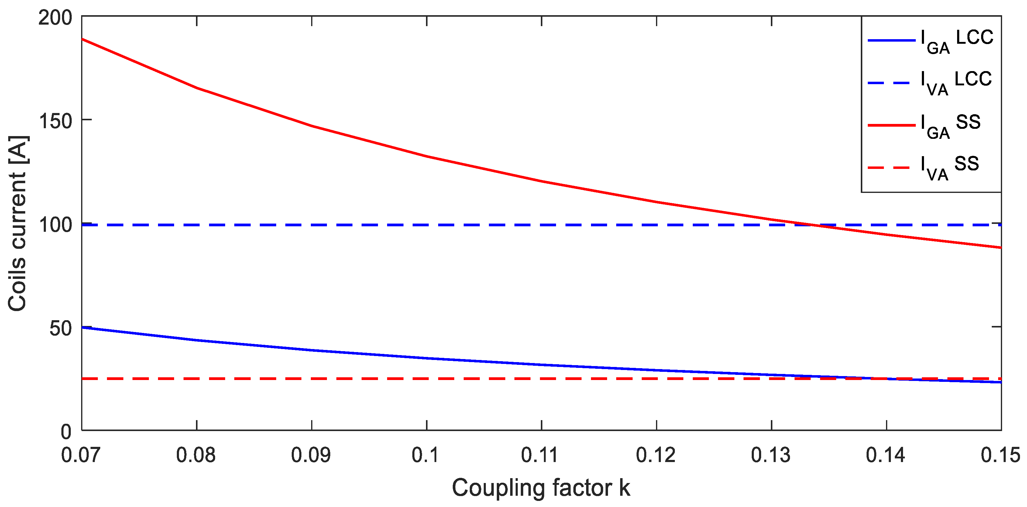
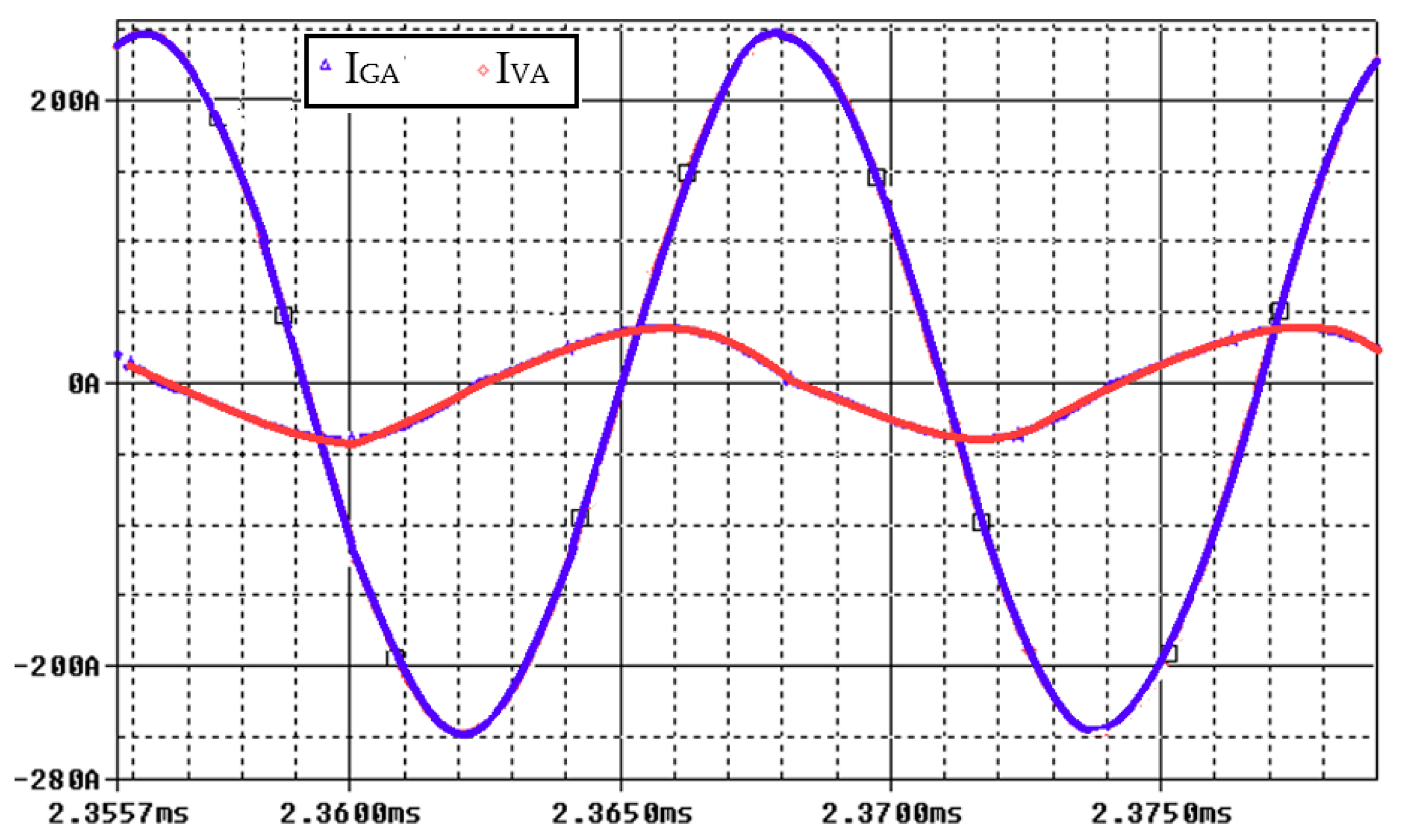
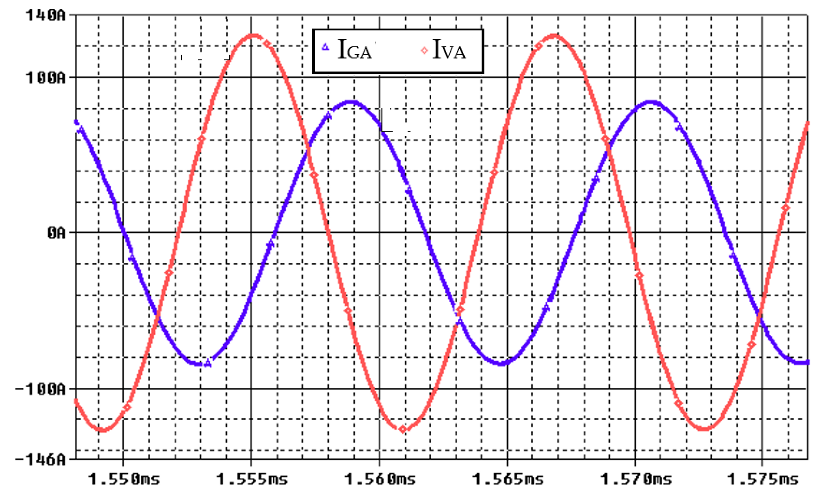
| 0.072 | 177.2 | 28.7 | 0.880 | 82 | 60.2 | 89.5 | 0.915 | 117 |
| 0.148 | 125.1 | 28.7 | 0.920 | 81 | 81.6 | 21.3 | 0.922 | 115 |
© 2019 by the authors. Licensee MDPI, Basel, Switzerland. This article is an open access article distributed under the terms and conditions of the Creative Commons Attribution (CC BY) license (http://creativecommons.org/licenses/by/4.0/).
Share and Cite
Campi, T.; Cruciani, S.; Maradei, F.; Feliziani, M. Magnetic Field during Wireless Charging in an Electric Vehicle According to Standard SAE J2954. Energies 2019, 12, 1795. https://doi.org/10.3390/en12091795
Campi T, Cruciani S, Maradei F, Feliziani M. Magnetic Field during Wireless Charging in an Electric Vehicle According to Standard SAE J2954. Energies. 2019; 12(9):1795. https://doi.org/10.3390/en12091795
Chicago/Turabian StyleCampi, Tommaso, Silvano Cruciani, Francesca Maradei, and Mauro Feliziani. 2019. "Magnetic Field during Wireless Charging in an Electric Vehicle According to Standard SAE J2954" Energies 12, no. 9: 1795. https://doi.org/10.3390/en12091795