Methodology for the Quantification of the Impact of Weather Forecasts in Predictive Simulation Models


Abstract
:1. Introduction
- MPC requires an optimization process that also has an inherent uncertainty. In [18], the authors have proposed a methodology to measure the accuracy of the optimization.
- Occupancy and user behavior, which is a stochastic and complex to be predicted parameter.
- Weather forecast that corresponds with the objective of this paper: the quantification of the weather forecasts’ errors and their effect on the indoor climate conditions and energy demand in a predictive energy model.
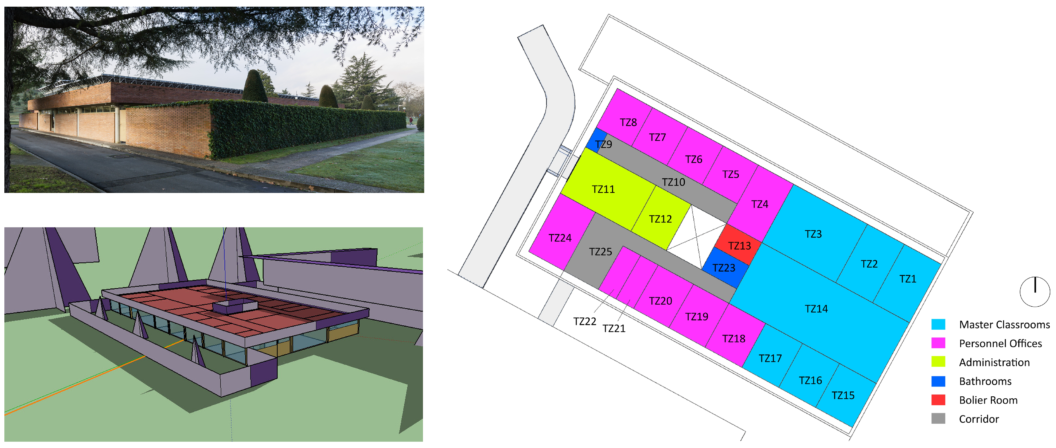
2. Test Site Description
3. Weather Data Processing
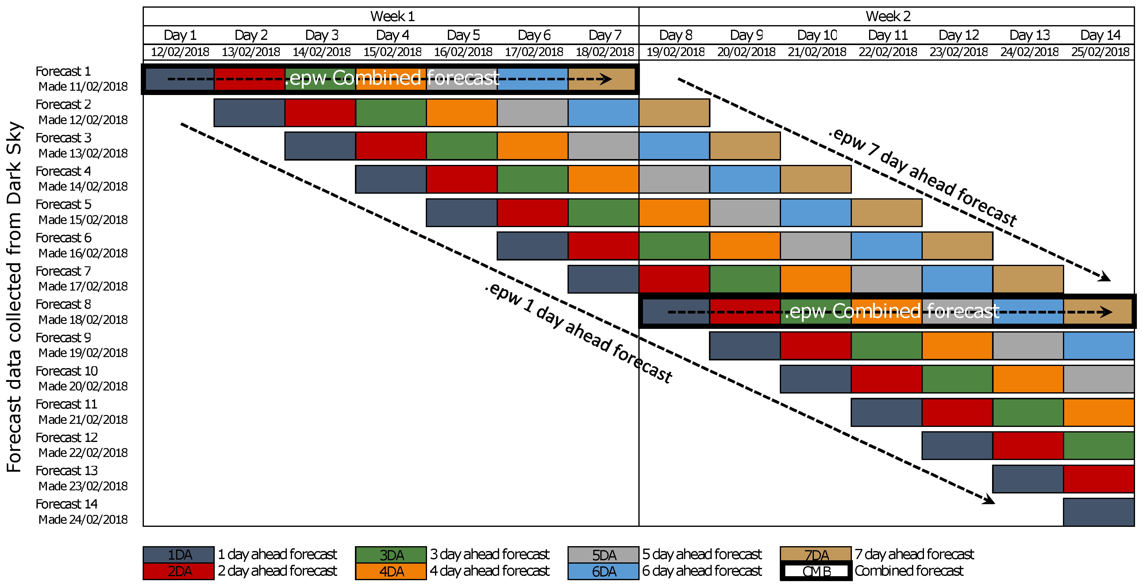
3.1. Weather Files Generation
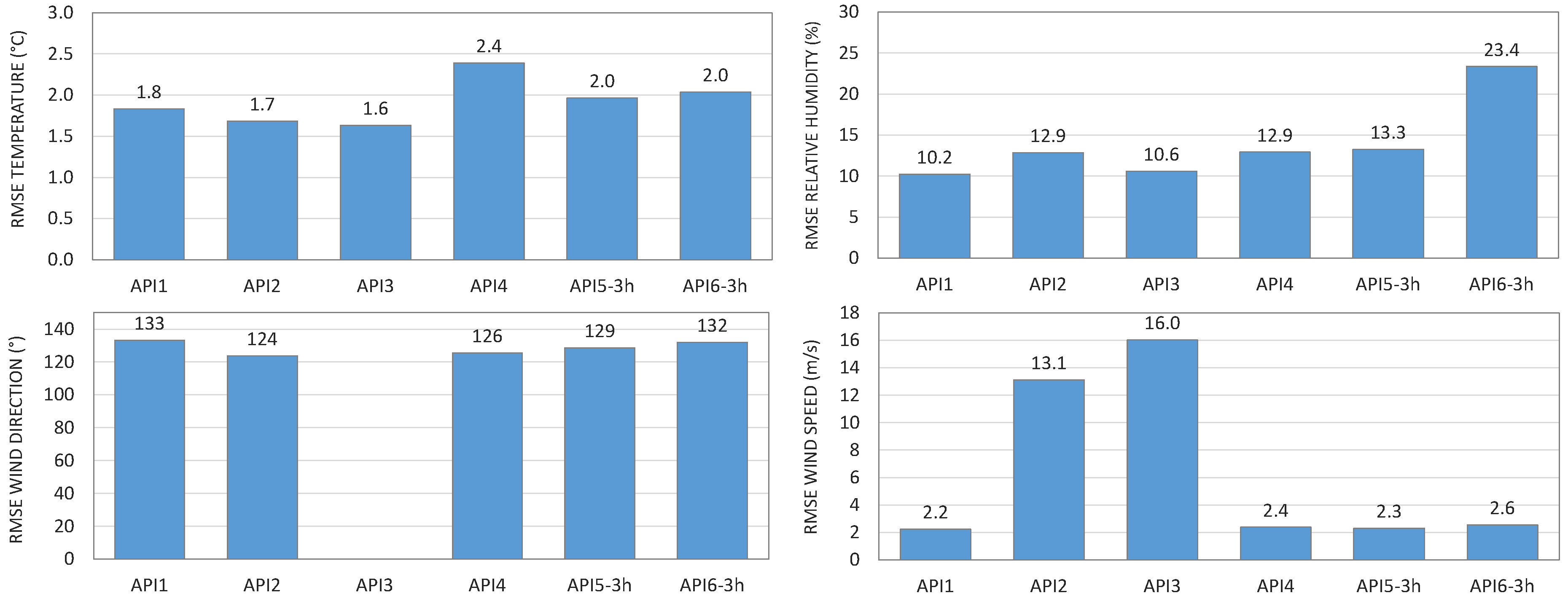
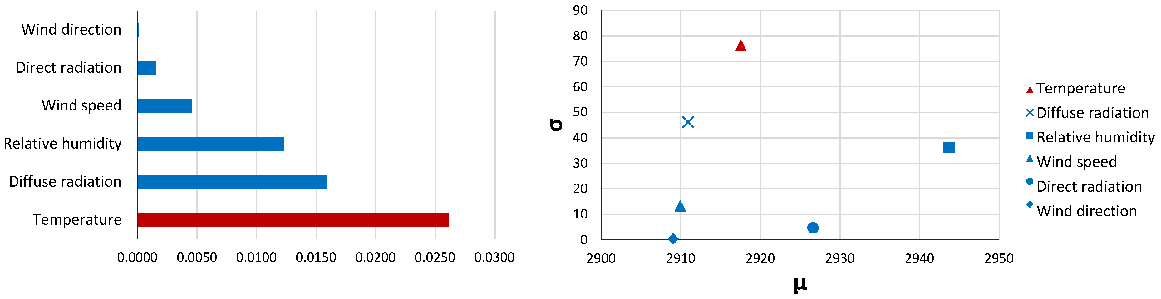
3.2. Sensitivity Analysis of Weather Parameters
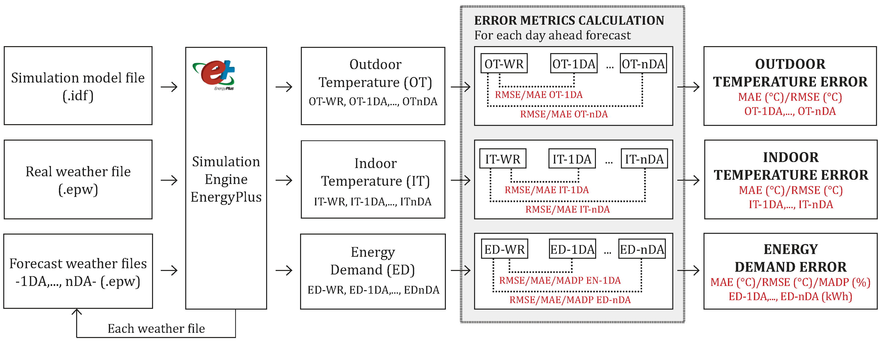
4. BEM Simulation and Error Metrics Calculation
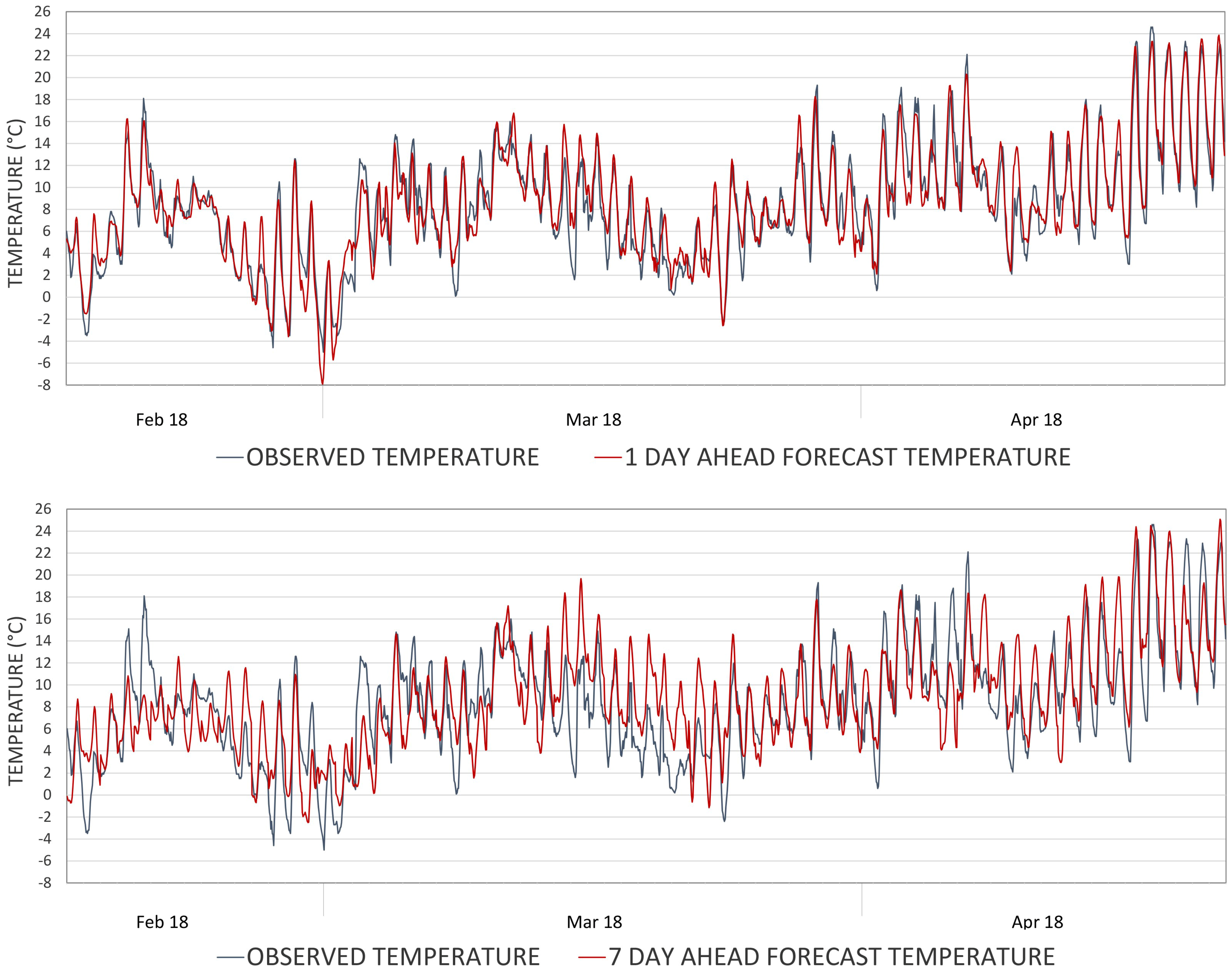
5. Analysis of the Results
6. Application of the Methodology: Model Predictive Control (MPC) for Building Energy Flexibility
7. Conclusions
Author Contributions
Funding
Acknowledgments
Conflicts of Interest
Abbreviations
| APIs | Application Programming Interfaces |
| ASHRAE | American Society of Heating, Refrigerating and Air-Conditioning Engineers |
| BEM | Building Energy Model |
| CMB | Combined Weather File |
| DA | Day-Ahead |
| ED | Energy Demand |
| EPW | EnergyPlus Weather File |
| FEMP | Federal Energy Management Program |
| HVAC | Heating, Ventilation and Air Conditioning |
| IDF | EnergyPlus Input Files |
| IPMVP | International Performance Measurement and Verification Protocol |
| IT | Mean Indoor Temperature |
| JSON | JavaScript Object Notation |
| kWh | Kilowatt Hour |
| MADP | Mean Absolute Deviation Percentage |
| MAE | Mean Absolute Error |
| MAPE | Mean Absolute Percentage Error |
| MARE | Mean Absolute Relative Error |
| MPC | Model Predictive Control |
| OT | Outdoor Temperature |
| REST | Representational State Transfer |
| RMSE | Root Mean Square Error |
| WR | Real Weather |
| XML | Extensible Markup Language |
References
- European Parliament, Directive 2012/27/EU of the European Parliament and of the Council of 25 October 2012 on energy efficiency, amending Directives 2009/125/EC and 2010/30/EU and repealing Directives 2004/8/EC and 2006/32/EC. Off. J. Eur. Union 2012, L, 1–56.
- Lazos, D.; Sproul, A.B.; Kay, M. Optimisation of energy management in commercial buildings with weather forecasting inputs: A review. Renew. Sustain. Energy Rev. 2014, 39, 587–603. [Google Scholar] [CrossRef]
- Jankovic, L. Designing resilience of the built environment to extreme weather events. Sustainability 2018, 10, 141. [Google Scholar] [CrossRef]
- Mohammadi, A.; Saghafi, M.R.; Tahbaz, M.; Nasrollahi, F. Effects of Vernacular Climatic Strategies (VCS) on Energy Consumption in Common Residential Buildings in Southern Iran: The Case Study of Bushehr City. Sustainability 2017, 9, 1950. [Google Scholar] [CrossRef]
- Petersen, S.; Svendsen, S. Method for simulating predictive control of building systems operation in the early stages of building design. Appl. Energy 2011, 88, 4597–4606. [Google Scholar] [CrossRef]
- OptiControl Project. Available online: http://opticontrol.ee.ethz.ch (accessed on 10 September 2018).
- Oldewurtel, F.; Parisio, A.; Jones, C.; Morari, M.; Gyalistras, D.; Gwerder, M.; Stauch, V.; Lehmann, B.; Wirth, K. Energy efficient building climate control using stochastic model predictive control and weather predictions. In Proceedings of the 2010 American Control Conference, Baltimore, MD, USA, 30 June–2 July 2010; IEEE Service Center: Piscataway, NJ, USA, 2010; pp. 5100–5105. [Google Scholar]
- Gyalistras, D.; Gwerder, M. Use of Weather and Occupancy Forecasts for Optimal Building Climate Control (OptiControl): Two Years Progress Report Main Report; Terrestrial Systems Ecology ETH Zurich R&D HVAC Products, Building Technologies Division; Siemens Switzerland Ltd.: Zug, Switzerland, 2010; p. 83. [Google Scholar]
- Sturzenegger, D.; Gyalistras, D.; Gwerder, M.; Sagerschnig, C.; Morari, M.; Smith, R.S. Model Predictive Control of a Swiss office building. In Proceedings of the Clima-Rheva World Congress, Prague, Czech Republic, 16–19 June 2013; pp. 3227–3236. [Google Scholar]
- Gwerder, M.; Gyalistras, D.; Sagerschnig, C.; Smith, R.; Sturzenegger, D. Final Report: Use of Weather and Occupancy Forecasts for Optimal Building Climate Control—Part II: Demonstration (OptiControl-II); Automatic Control Laboratory, ETH Zurich: Zug, Switzerland, 2013; p. 156. [Google Scholar]
- Cigler, J.; Gyalistras, D.; Široky, J.; Tiet, V.; Ferkl, L. Beyond theory: The challenge of implementing model predictive control in buildings. In Proceedings of the 11th Rehva World Congress, Clima, 2013, Prague, Czech Republic, 16–19 June 2013; Volume 250. [Google Scholar]
- Jensen, S.; Marszal-Pomianowska, A.; Lollini, R.; Pasut, W.; Knotzer, A.; Engelmann, P.; Stafford, A.; Reynders, G. IEA EBC annex 67 energy flexible buildings. Energy Build. 2017, 155, 25–34. [Google Scholar] [CrossRef]
- Hedegaard, R.E.; Pedersen, T.H.; Petersen, S. Multi-market demand response using economic model predictive control of space heating in residential buildings. Energy Build. 2017, 150, 253–261. [Google Scholar] [CrossRef]
- Heidrich, T.; Grobe, J.; Meschede, H.; Hesselbach, J. Economic Multiple Model Predictive Control for HVAC Systems—A Case Study for a Food Manufacturer in Germany. Energies 2018, 11, 3461. [Google Scholar] [CrossRef]
- Ruiz, G.R.; Bandera, C.F.; Temes, T.G.A.; Gutierrez, A.S.O. Genetic algorithm for building envelope calibration. Appl. Energy 2016, 168, 691–705. [Google Scholar] [CrossRef]
- Ruiz, G.R.; Bandera, C.F. Analysis of uncertainty indices used for building envelope calibration. Appl. Energy 2017, 185, 82–94. [Google Scholar] [CrossRef]
- Fernández Bandera, C.; Ramos Ruiz, G. Towards a New Generation of Building Envelope Calibration. Energies 2017, 10, 2102. [Google Scholar] [CrossRef]
- Ramos Ruiz, G.; Lucas Segarra, E.; Fernández Bandera, C. Model Predictive Control Optimization via Genetic Algorithm Using a Detailed Building Energy Model. Energies 2019, 12, 34. [Google Scholar] [CrossRef]
- Sandels, C.; Widén, J.; Nordström, L.; Andersson, E. Day-ahead predictions of electricity consumption in a Swedish office building from weather, occupancy, and temporal data. Energy Build. 2015, 108, 279–290. [Google Scholar] [CrossRef]
- Hossa, T.; Filipowska, A.; Fabisz, K. The comparison of medium-term energy demand forecasting methods for the need of microgrid management. In Proceedings of the 2014 IEEE International Conference on Smart Grid Communications (SmartGridComm), Venice, Italy, 3–6 November 2014; pp. 590–595. [Google Scholar]
- Yuce, B.; Mourshed, M.; Rezgui, Y. A smart forecasting approach to district energy management. Energies 2017, 10, 1073. [Google Scholar] [CrossRef]
- Agüera-Pérez, A.; Palomares-Salas, J.C.; de la Rosa, J.J.G.; Florencias-Oliveros, O. Weather forecasts for microgrid energy management: Review, discussion and recommendations. Appl. Energy 2018, 228, 265–278. [Google Scholar] [CrossRef]
- Henze, G.P.; Kalz, D.E.; Felsmann, C.; Knabe, G. Impact of forecasting accuracy on predictive optimal control of active and passive building thermal storage inventory. HVAC&R Res. 2004, 10, 153–178. [Google Scholar]
- Oldewurtel, F.; Parisio, A.; Jones, C.N.; Gyalistras, D.; Gwerder, M.; Stauch, V.; Lehmann, B.; Morari, M. Use of model predictive control and weather forecasts for energy efficient building climate control. Energy Build. 2012, 45, 15–27. [Google Scholar] [CrossRef] [Green Version]
- Zhao, J.; Liu, X. A hybrid method of dynamic cooling and heating load forecasting for office buildings based on artificial intelligence and regression analysis. Energy Build. 2018, 174, 293–308. [Google Scholar] [CrossRef]
- Du, H.; Jones, P.; Ng, B. Understanding the reliability of localized near future weather data for building performance prediction in the UK. In Proceedings of the 2016 IEEE International Smart Cities Conference (ISC2), Trento, Italy, 12–15 September 2016; pp. 1–4. [Google Scholar]
- Du, H.; Barclay, M.; Jones, P. Generating High Resolution Near-Future Weather Forecasts for Urban Scale Building Performance Modelling. In Proceedings of the Building Simulation 2017: 15th Conference of International Building Performance Simulation Association, San Francisco, CA, USA, 7–9 August 2017. [Google Scholar]
- Du, H.; Segarra, E.L.; Bandera, C.F. Development of a REST API for obtaining site-specific historical and near-future weather data in EPW format. In Proceedings of the BSO 2018 4th Building Simulation and Optimization Conference, Cambridge, UK, 11–12 September 2018. [Google Scholar]
- Conejo, A.J.; Sioshansi, R. Rethinking restructured electricity market design: Lessons learned and future needs. Int. J. Electr. Power Energy Syst. 2018, 98, 520–530. [Google Scholar] [CrossRef]
- Péan, T.Q.; Torres, B.; Salom, J.; Ortiz, J. Representation of daily profiles of building energy flexibility. In Proceedings of the eSim, Montréal, QC, Canada, 9–10 May 2018. [Google Scholar]
- Guglielmetti, R.; Macumber, D.; Long, N. OpenStudio: An open source integrated analysis platform. In Proceedings of the 12th Conference of International Building Performance Simulation Association, Sydney, Australia, 14–16 November 2011. [Google Scholar]
- Crawley, D.B.; Lawrie, L.K.; Winkelmann, F.C.; Buhl, W.F.; Huang, Y.J.; Pedersen, C.O.; Strand, R.K.; Liesen, R.J.; Fisher, D.E.; Witte, M.J.; et al. EnergyPlus: Creating a new-generation building energy simulation program. Energy Build. 2001, 33, 319–331. [Google Scholar] [CrossRef]
- Crawley, D.B.; Lawrie, L.K.; Pedersen, C.O.; Winkelmann, F.C.; Witte, M.J.; Strand, R.K.; Liesen, R.J.; Buhl, W.F.; Huang, Y.J.; Henninger, R.H.; et al. EnergyPlus: An update. Proc. SimBuild 2004, 1, 1–8. [Google Scholar]
- Recast, E. Directive 2010/31/EU of the European Parliament and of the Council of 19 May 2010 on the energy performance of buildings (recast). Off. J. Eur. Union 2010, 18, 2010. [Google Scholar]
- IPMVP Committee. International Performance Measurement and Verification Protocol: Concepts and Options for Determining Energy and Water Savings; Technical Report; National Renewable Energy Lab.: Golden, CO, USA, 2001; Volume I.
- FEMP, M. Guidelines: Measurement and Verification for Federal Energy Projects; Version 3.0.; Energy Efficiency and Renewable Energy: Washington, DC, USA, 2008.
- FEMP, M. Guidelines: Measurement and Verification for Federal Energy Projects; Version 4.0; Energy Efficiency and Renewable Energy: Washington, DC, USA, 2015.
- ASHRAE. Guideline 14-2002, Measurement of Energy and Demand Savings; ASHRAE: Atlanta, GA, USA, 2002; p. 22. [Google Scholar]
- Ruiz, G.R.; Bandera, C.F. Validation of Calibrated Energy Models: Common Errors. Energies 2017, 10, 1587. [Google Scholar] [CrossRef]
- del Estado, Boletín Oficial. Real Decreto 1027/2007, Reglamento de Instalaciones Térmicas en los Edificios (RITE). 2007. Available online: https://www.iberley.es/legislacion/real-decreto-1027-2007-20-jul-reglamento-instalaciones-termicas-edificios-4817359 (accessed on 10 September 2018).
- DOE, E. Auxiliary Programs: EnergyPlusTM Version 8.9.0 Documentation; US Department of Energy: Washington, DC, USA, 2018.
- AEMET, Agencia Estatal de Meteorología. Available online: http://aemet.es (accessed on 10 September 2018).
- Meteorologisk Institutt. Available online: https://api.met.no (accessed on 10 September 2018).
- Open Weather Map. Available online: https://openweathermap.org/api (accessed on 10 September 2018).
- Weatherbit.io. Available online: https://www.weatherbit.io/api (accessed on 10 September 2018).
- The Dark Sky Company, LLC. Available online: https://darksky.net/dev (accessed on 10 September 2018).
- Weather Underground. Available online: https://www.wunderground.com/weather/api/ (accessed on 10 September 2018).
- Dimas, F.; Gilani, S.; Aris, M. Hourly solar radiation estimation from limited meteorological data to complete missing solar radiation data. In Proceedings of the International Conference on Enviroment Science and Engineering IPCBEE, Singapore, 26–28 February 2011; Volume 2628, p. 48. [Google Scholar]
- Spokas, K.; Forcella, F. Estimating hourly incoming solar radiation from limited meteorological data. Weed Sci. 2006, 54, 182–189. [Google Scholar] [CrossRef]
- Morris, M.D. Factorial sampling plans for preliminary computational experiments. Technometrics 1991, 33, 161–174. [Google Scholar] [CrossRef]
- Hamby, D. A review of techniques for parameter sensitivity analysis of environmental models. Environ. Monit. Assess. 1994, 32, 135–154. [Google Scholar] [CrossRef] [PubMed] [Green Version]
- Zhao, J.; Duan, Y.; Liu, X. Uncertainty Analysis of Weather Forecast Data for Cooling Load Forecasting Based on the Monte Carlo Method. Energies 2018, 11, 1900. [Google Scholar] [CrossRef]
- Mirakyan, A.; Meyer-Renschhausen, M.; Koch, A. Composite forecasting approach, application for next-day electricity price forecasting. Energy Econ. 2017, 66, 228–237. [Google Scholar] [CrossRef]
- Petojević, Z.; Gospavić, R.; Todorović, G. Estimation of thermal impulse response of a multi-layer building wall through in-situ experimental measurements in a dynamic regime with applications. Appl. Energy 2018, 228, 468–486. [Google Scholar] [CrossRef]


| API Provider | Forecast | Interval | Format |
|---|---|---|---|
| aemet [42] | Next 7-day | hourly | JSON |
| met.no [43] | Next 10-day | hourly | XML |
| openweathermap [44] | Next 5-day | 3-hourly | XML/ JSON |
| weatherbit [45] | Next 5-day | 3-hourly | JSON |
| dark sky [46] | Next 7-day | hourly | JSON |
| wunderground [47] | Next 10-day | hourly | XML/ JSON |
| Parameter | Index | 1DA | 2DA | 3DA | 4DA | 5DA | 6DA | 7DA | CMB |
|---|---|---|---|---|---|---|---|---|---|
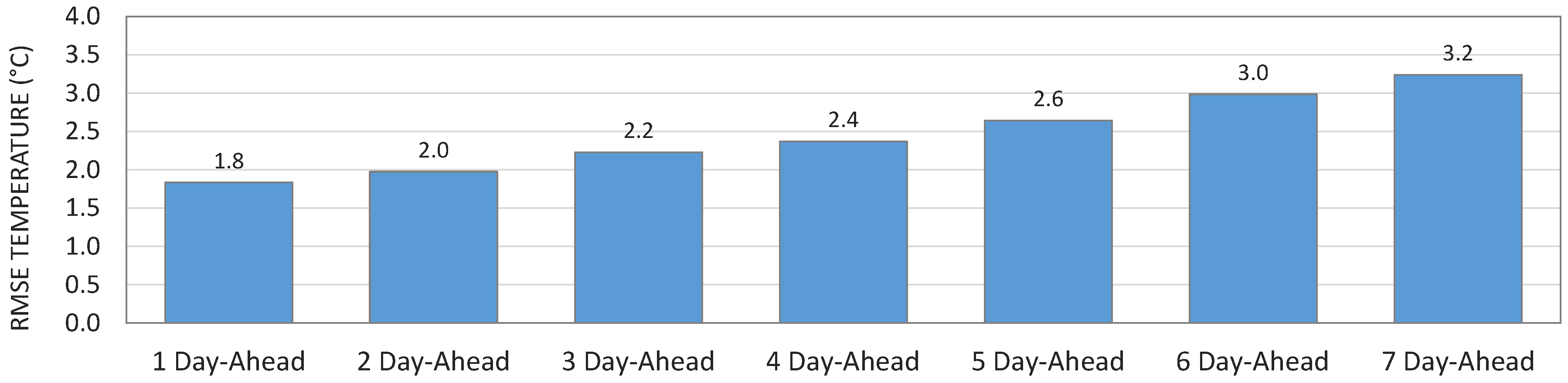
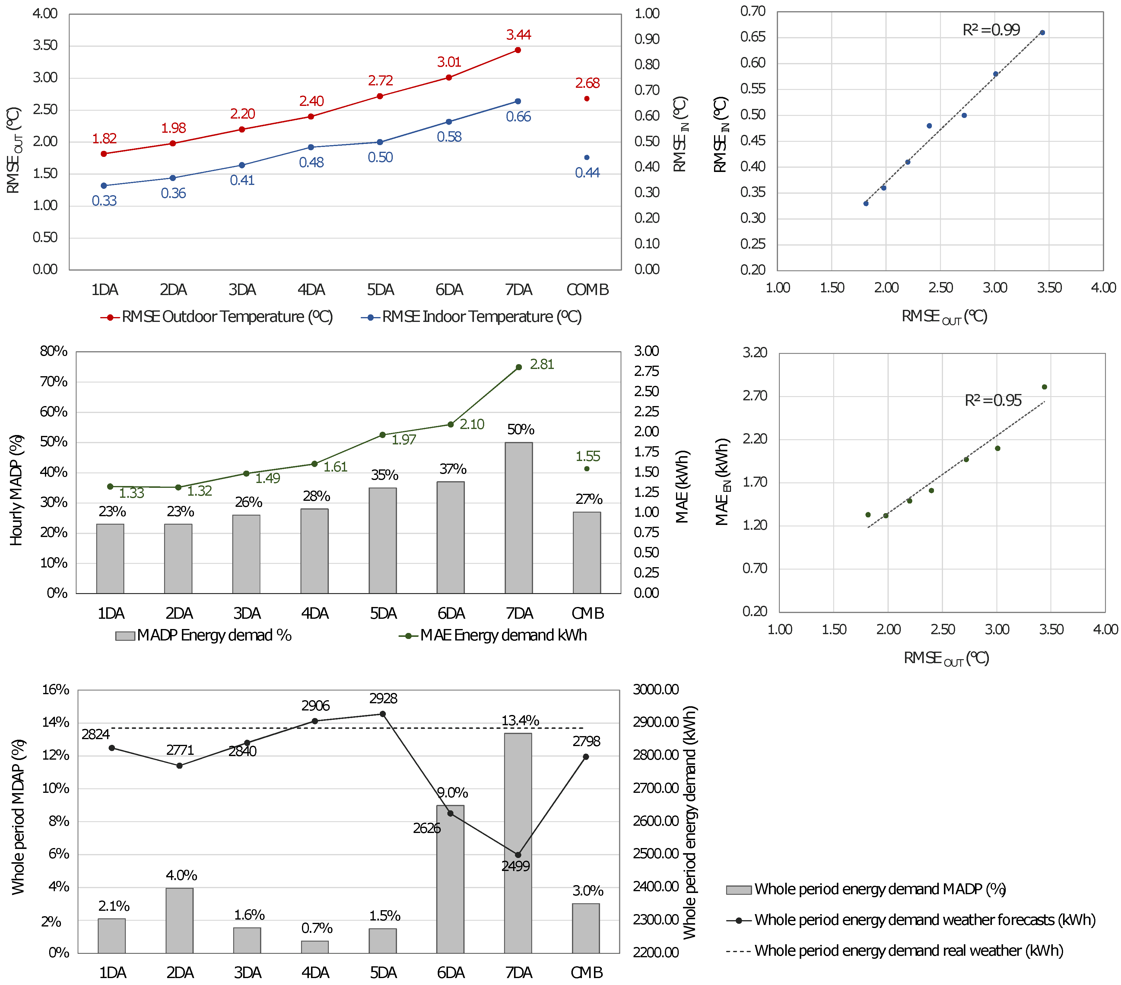
| Outdoor temperature | (C) | 1.82 | 1.98 | 2.2 | 2.4 | 2.72 | 3.01 | 3.44 | 2.68 |
| (C) | 1.39 | 1.55 | 1.73 | 1.88 | 2.14 | 2.34 | 2.68 | 2.1 | |
| Indoor temperature | (C) | 0.33 | 0.36 | 0.41 | 0.48 | 0.5 | 0.58 | 0.66 | 0.44 |
| (C) | 0.25 | 0.28 | 0.32 | 0.37 | 0.39 | 0.44 | 0.54 | 0.33 | |
| Energy Demand | (kWh) | 1.74 | 1.73 | 1.92 | 2.11 | 2.51 | 2.91 | 3.44 | 2.04 |
| (kWh) | 1.33 | 1.32 | 1.49 | 1.61 | 1.97 | 2.1 | 2.81 | 1.55 | |
| (%) | 23 | 23 | 26 | 28 | 35 | 37 | 50 | 27 |
© 2019 by the authors. Licensee MDPI, Basel, Switzerland. This article is an open access article distributed under the terms and conditions of the Creative Commons Attribution (CC BY) license (http://creativecommons.org/licenses/by/4.0/).
Share and Cite
Lucas Segarra, E.; Du, H.; Ramos Ruiz, G.; Fernández Bandera, C. Methodology for the Quantification of the Impact of Weather Forecasts in Predictive Simulation Models. Energies 2019, 12, 1309. https://doi.org/10.3390/en12071309
Lucas Segarra E, Du H, Ramos Ruiz G, Fernández Bandera C. Methodology for the Quantification of the Impact of Weather Forecasts in Predictive Simulation Models. Energies. 2019; 12(7):1309. https://doi.org/10.3390/en12071309
Chicago/Turabian StyleLucas Segarra, Eva, Hu Du, Germán Ramos Ruiz, and Carlos Fernández Bandera. 2019. "Methodology for the Quantification of the Impact of Weather Forecasts in Predictive Simulation Models" Energies 12, no. 7: 1309. https://doi.org/10.3390/en12071309