Multi-Period Observation Clustering for Tariff Definition in a Weekly Basis Remuneration of Demand Response

Abstract

Distributed energy resources can improve the operation of power systems, improving economic and technical efficiency. Aggregation of small size resources, which exist in large number but with low individual capacity, is needed to make these resources’ use more efficient. In the present paper, a methodology for distributed resources management by an aggregator is proposed, which includes the resources scheduling, aggregation and remuneration. The aggregation, made using a k-means algorithm, is applied to different approaches concerning the definition of tariffs for the period of a week. Different consumer types are remunerated according to time-of-use tariffs existing in Portugal. Resources aggregation and remuneration profiles are obtained for over 20.000 consumers and 500 distributed generation units. The main goal of this paper is to understand how the aggregation phase, or the way that is performed, influences the final remuneration of the resources associated with Virtual Power Player (VPP). In order to fulfill the proposed objective, the authors carried out studies for different time frames (week days, week-end, whole week) and also analyzed the effect of the formation of the remuneration tariff by considering a mix of fixed and indexed tariff. The optimum number of clusters is calculated in order to determine the best number of DR programs to be implemented by the VPP.

1. Introduction

The concept of Demand Response (DR) introduced a new role for consumers in the grid. Becoming more active agents, end-users can reduce demand according to technical or economic problems or even in response to price signals and incentives, having more information about what is happening in the network infrastructure [1,2,3,4]. DR programs focus mostly on large-size resources despite recent efforts to highlight small-size ones as well. The last ones will only be useful if they provide a coordinated response with more resources of this kind. Thus, one of the solutions is to establish an aggregating entity. Through this approach, the aggregator would participate in wholesale electricity markets as an intermediary in the transactions between this group of consumers and independent system operator (ISO) [5,6].

DR will have influence on different system costs and may increase the reliability of the system. By increasing network flexibility supported by bi-directional communications in the system, it will enable higher levels of penetration of small renewable energy resources [7,8]. In this context, it is also necessary to aggregate Distributed Generation (DG) units. With a larger integration of different resource types, a Virtual Power Player (VPP) is a commonly known aggregator, being responsible for the management of the small resources [9,10].

An aggregator can also play a crucial role in the system since the high penetration of these less predictable features in the current network can cause an imbalance between supply and demand if they are not managed in the best way [11,12]. By controlling these resources, the aggregator performs an optimal scheduling to meet the demands of the loads, enabling their participation in the electricity markets. The aggregator is also responsible for the fair remuneration of aggregate resources—this task is crucial since it represents an incentive for the continued participation of consumers and producers in network management. Thus, it is important to find adequate methods and tools that support the aggregator in the accomplishment of the aggregation—since this will be this way of forming the groups of resources, becomes a subject of high importance.

Several authors have described clustering algorithms to perform resources aggregation. Given a database, these algorithms can form groups by identifying common characteristics or patterns between elements [13]. There are different clustering algorithms, namely, partitioning, fuzzy, hierarchical, density-based, model-based and more. In the present paper, the authors opted for one of the most popular methods of clustering—k-means—which has proved also to be accurate in the aggregation of resources for their remuneration. This algorithm, proposed by Hartigan-Wong in 1979, defines that at each iteration the distance between the points in the database and the center of each group is calculated to form the groups. In other words, the total variation within a cluster is then taken to the sum of the squares of Euclidean distance between a point and the center of the cluster, and then assigns the point to the nearest cluster [14].

Going forward, the methodology proposed in the present paper addresses the study of different time periods—week, weekend and full week—comparing and perceiving the different situations by finding solutions that may be useful for the aggregator. Moreover, the proposed methodology includes small resources participation in the market. Although the analysis is focused only on consumers of Incentive-based Demand Response program (IDR), other DR programs as well as DG units or even prosumers—consumers that have the possibility to produce—can be used in the proposed methodology, making it flexible enough to be used by any type of aggregator. In addition, the remuneration is made in a fair way even for the least efficient resources and at the same time can encourage the others to continue to be associated with this aggregator. The proposed approach supports the aggregator performing the schedule of the aggregated resources, aggregating resources by clustering the related data, and remunerating the resources according to the actual participation. Through an optimization, resources will be optimally scheduled in order to minimize operating costs. The remuneration tariff will be found, paying all the resources of the given group at the same rate.

The paper is organized in five sections. After the introduction, Section 2 provides the literature review, and Section 3 presents the methodology proposed in a detailed way. Section 4 presents the case study which results are presented in Section 5. Finally, Section 6 presents the conclusions.

2. Related Literature

The remuneration of resources is usually made equally for the resources of the same type. However, this task can be done individually, depending on the contribution of each element. In fact, in the aggregator operation context, the aggregation and remuneration of the resources is largely related to the scheduling of resources.

In [15] an approach is presented to determine an optimal incentive rate for incorporating large industries in demand response programs, focusing on the reality of Iran. Other related works consider the aggregation of resources for different time periods, namely in smart grids. In [16] an optimization model is proposed to determine the optimal operation of a DR aggregator that manages the portfolio of DR resources based on bilateral contracts of different characteristics to participate in day-ahead and real-time markets. In [17], an optimal day-ahead scheduling of isolated microgrid with an electric vehicle battery swapping station in multi-stakeholder scenarios was investigated. An initial version of the proposed methodology was developed for a single period in [18].

In [19] a decentralized framework in which the aggregator seeks to maximize its profits while the consumers minimize their costs in response to time-varying prices, and additional incentives provided to mitigate potential overloads in the distribution system is proposed. In [20], a Cournot game model is proposed taking into account generation resource providers, ISO and DR aggregators—the solution is developed for the wholesale market with DR aggregators.

Looking for a layered model of DR participation with load aggregators operating as media, in [21] a model in which the target is to develop the solution to a multi-objective optimization problem based on the assumption that the market with participation of DR resources is completely competitive is built.

While in [22] the aim is to manage the electrical energy in unbalanced distribution networks in order to minimize the annual energy purchased from substation, in [23] a generic demand model that captures the aggregated effect of a large population of prosumers equipped with small-scale PV-battery systems, that behave in the same way and have the same capacity, is proposed.

In [24,25], the authors of the present paper proposed different methodologies for the consumers and distributed generation aggregation and remuneration supported by distinct clustering algorithms in a single period.

Providing innovative improvements from the previous literature, in order to propose a methodology that gives better results for the problem of aggregation and remuneration, in comparison to the referred works, in the present paper, both large and small size resources and prosumers were incorporated. It should be noted that the proposed methodology can handle a small database, as well as one with thousands of resources. Also, regarding the time horizon of handled scenarios, a multiperiod optimization is included in the proposed methodology. Moreover, instead of providing a single optimal solution, which is sometimes very limiting for the aggregator (VPP), the goal is to provide the VPP with different solutions in order to perceive which one suits better in the situation that this entity is facing. Instead of assuming that the participation of DR is fully competitive, the proposed methodology deals with the aggregation and remuneration of associated resources, trying the find the fair tariff, in addition to optimal scheduling. Also, it is assumed that the VPP aggregates consumers or DG units or the mixture of the two, making it quite flexible in this matter. In this way, in addition to consider prosumers with different systems, consumers and producers in the same aggregation, it is also considered that they can behave in different ways and don’t have the same capacity.

Overall, the proposed methodology is advantageous in reducing the operation costs for the VPP while providing adequate remuneration to the participating consumers, DG units, and prosumers, providing decision on the best number of clusters to be adopted, and the set of days to be aggregated in the definition of tariffs.

3. Proposed Methodology

The main question to be answered by the proposed methodology is: is it worth to define different tariffs for week days and weekends or a tariff for the complete week is adequate?

The proposed methodology, according to Figure 1, implements distinct phases in order to support the decisions of the aggregator in what concerns fair remuneration. Since it is assumed that the aggregator is an independent entity, and also that the resources have signed a contract with this entity, the aggregated resources are assumed to respond to DR events whenever requested. With the proposed methodology, the authors emphasize the following as innovative contributions in relation to previous works discussed in Section 2:

• Inclusion of prosumers in the aggregation and remuneration of resources, as being consumers and producers at the same time they have specific characteristics while providing load reduction in demand response programs;
• Bounding of each resource participation in the obtained schedule, namely for consumers, producers, and prosumers, by implementing α in the formulation of the optimization problem;
• Creation of DR and tariff groups that put together small-size and medium-size resources in the same group according to the actual characteristics of response;
• Definition of a fair remuneration of consumers, producers and prosumers, according to their actual performance instead of grouping resources in the same tariff according to size and rated power characteristics;
• The optimization and aggregation are done for a set of consecutive days, instead of considering only a complete day analysis, day-by-day. In this way, the tariffs definition is made according to the performance of each resource or consumer in the whole set of days, distinguishing week days and week-end days;
• The formation of the remuneration tariff is made as a mix of fixed and indexed tariff. In this way, the resources know that part of the remuneration is ensured as contracted but the other part is taking into account the market prices, making it possible for the VPP to share the risks and benefits of the changing prices in the market;
• The discussion of the seasonality of tariffs along the week and along the day for different consumers, adding more variability and interest on the proposed aggregation scheme;
• Easily scalable in order to accomplish the schedule, aggregation, and remuneration of a large number of resources and consumers. A limitation can exist at the hardware level in order to compute all the data. Also, the required time to obtain results will not be a problem since the developed methodology is driven to be run in a day-ahead or hour-ahead configuration.
• The optimum number of clusters is discussed and compared to the ideal number of clusters that are targeted by the VPP. In this way, the VPP is able to determine the best number of DR programs to be implemented.
• Wind generation is modeled taking into account the cut-in and cut-out wind speed.

Thus, the present methodology aims to minimize operating costs, at optimally scheduling resources, and at defining aggregation and remuneration.

The proposed method considers resources as suppliers, DG units, and consumers enrolled in DR programs. Consumers may belong to IDR programs, where they are proportionately remunerated according to their contribution to reducing the overall load. Figure 1 presents a general diagram of the proposed methodology, showing the four phases: the definition of the input data, the optimum scheduling, the aggregation phase of the resources and the definition of the remuneration tariffs for each group.

In a first phase, the input data is collected, these being the characteristics that define the resources associated with this aggregator, namely the maximum capacity of the DG units, the suppliers and the reduction capacity of the consumers belonging to programs of DR, as well as the consumption tariffs associated with each resource.

Then, the optimal scheduling is performed. The objective function of the optimization problem is presented in Equation (1) and aims to minimize operating costs:

$$\begin{array}{c}MinOC={\displaystyle \sum _{p=1}^P}{P}_{DG\left(p\right)}\times C_{DG\left(p\right)}+P_{NSP}\times C_{NSP}+{\displaystyle \sum _{s=1}^S}\left[\begin{array}{c}{P}_{Sup\left(s\right)}^{}\times C_{Sup\left(s\right)}^{}\\ \end{array}\right]\\ +{\displaystyle \sum _{c=1}^C}\left[\begin{array}{c}{P}_{IDR\left(c\right)}\times C_{IDR\left(c\right)}\\ \end{array}\right]\end{array}$$

(1)

In the objective function (1) multiple resources are considered, such as DG units, consumers belonging to DR programs, those belonging to IDR and also external suppliers. The suppliers are considered in the hypothesis that the aggregate production resources do not satisfy the needs of the demand and so they can cooperate to find the balance point of the network. By placing the suppliers at different prices, they will be activated as needed. The optimization constraints are presented in Equations (2)–(10). Equation (2) represents the power balance equation:

$${\displaystyle \sum _{c=1}^C}\left[P_{Load\left(c\right)}^{Initial}-P_{IDR\left(c\right)}\right]={\displaystyle \sum _{p=1}^P}{P}_{DG\left(p\right)}+{\displaystyle \sum _{s=1}^S}{P}_{Sup\left(s\right)}^{}+P_{NSP}$$

(2)

It is imperative that the balance between demand and supply be accomplished. Equation (2) shows that the initial consumption should be deducted from the possible reduction of each IDR consumer and that this value should equal the sum of all DG units and suppliers. Also included in this equation is the value for Non-Supplied Power (NSP). This value is the amount of load lost if the total production fails to supply the demand.

Equations (3) and (4) represent the technical limits for external suppliers. Equations (3) and (4) refer to suppliers, presenting the upper limit and the limit for the total quantity brought by this type of supplier:

$$P_{Supplier(s)}^{reg}\le P_{Supplier(s)}^{regMax},\forall s\in \left\{1,\dots ,S\right\}$$

(3)

$${\displaystyle \sum _{s=1}^S{P}_{Supplier(s)}^{reg}}\le P_{Supplier}^{regTotal}$$

(4)

Regarding to equations (5) and (6), these present the technical limits for DG units:

$$P_{DG(p)}^{}\le P_{DG(p)}^{Max},\forall p\in \left\{1,\dots ,P\right\}$$

(5)

$${\displaystyle \sum _{p=1}^P{P}_{DG(p)}^{}}\le P_{DG}^{TotalMax}$$

(6)

In order to realize the amount of the power available from wind, Equation (7) has been implemented [26]:

$$P_{DG}^{Wind}=\frac{1}{2}{\rho }_{air}\pi r^2{v}^3{C}_p$$

(7)

Equation (8) shows the maximum limit of each of the IDR providers:

$$P_{IDR(c)}^{}\le P_{IDR(c)}^{Max},\forall c\in \left\{1,\dots ,C\right\}$$

(8)

Equations (9)–(11) present the formulation of the DR program model for the consumers and their appliances:

$$P_{IDR(c)}^{}={\displaystyle \sum _{a=1}^{A_c}{\rho }_{a,c}^{}{\theta }_{a,c}^{}}$$

(9)

$${\rho }_{a,c}^{}\ge {\rho }_{a,c}^{\min }$$

(10)

$${\rho }_{a,c}^{}\le {\rho }_{a,c}^{\max }$$

(11)

Regarding Equations (12) and (13), a usage limitation constraint to enable control over the contribution of DG (α_DG) and IDR (α_IDR) is shown:

$$\frac{{\sum }_{p=1}^P{P}_{DG\left(p\right)}}{{\sum }_{s=1}^S\left[\begin{array}{c}{P}_{Supplier\left(s\right)}^{reg}\\ +P_{Supplier\left(s\right)}^{add}\end{array}\right]+{\sum }_{p=1}^P{P}_{DG\left(p\right)}+{\sum }_{c=1}^C\left[P_{IDR\left(c\right)}\right]+P_{NSP}}\le {\alpha }_{DG}$$

(12)

$$\frac{{\sum }_{c=1}^C{P}_{IDR\left(c\right)}}{{\sum }_{s=1}^S\left[\begin{array}{c}{P}_{Supplier\left(s\right)}^{reg}\\ +P_{Supplier\left(s\right)}^{add}\end{array}\right]+{\sum }_{p=1}^P{P}_{DG\left(p\right)}+{\sum }_{c=1}^C\left[P_{IDR\left(c\right)}\right]+P_{NSP}}\le {\alpha }_{IDR}$$

(13)

The α parameters can take values between 0 and 1. Equations (12) and (13) provide the VPP with an additional tool to manage the resources, considering its operation context and/or other constraints. For example, for α_DG equal to 0.3, it will result a contribution of DG resources to supply the demand lower or equal to 30%.

Returning to the methodology proposed by the authors, now is presented the third phase—the aggregation of resources, which is the main focus of this paper. In this way, the authors choose a method of partitioning clustering—k-means—to perform the aggregation. In this method, it is necessary to find a centroid value to represent each group. This value is found when the distance value of these elements for the remaining elements of the group is minimal. Several functions can be used to calculate the minimum distance between elements. In the paper in question Euclidean distance represented in Equation (14) was used:

$$d\left(x,c\right)=\left(x-c\right){\left(x-c\right)}^{\prime }$$

(14)

The aggregation is done separately for each type of aggregated resource, namely DG and IDR. As the selected method (k-means) allows one to consider several observations of the variables under study, it was possible to aggregate all information—different periods of time— in the same input matrix. In this way, variables go to rows and the different periods in columns. Thus, it is possible to form a standardized group and not concentrated as when hierarchical clustering algorithms are used. The result displays all resources, and to which group they belong. Throughout this phase, it will be necessary to define a range for the parameter k that results in the number of groups that the k-means method will form.

The optimal number of clusters for a given database can be determined. There are several methods for this purpose, for example the Elbow Method and the Silhouette Method. The first, the Elbow Method, is a visual method and is one of the oldest methods. Starting with k = 2 and incrementing in a step of 1, the clustering method is applied and the cost that comes with this training is found. Upon reaching a k where the cost value decreases drastically and then hits a plateau, the optimal k was found, [27]. Regarding the Silhouette Method, the silhouette value for each point is measured by the similarity that this point has with the remaining points of its cluster when compared to other clusters. Thus, the silhouette of a cluster is a graph with the silhouette value for all points in the database. To compare between clusters is used average silhouette width (ASW) of a cluster and the optimal value of k will be one in which the value of ASW is maximum [28]. However, it is worth remembering that the optimum number of clusters may not be the ideal clusters value for a given situation. This methodology gives the VPP the freedom to study different cases and to see which is the best and the most appropriate.

Phase four of the proposed methodology refers to the remuneration of resources. In the case of consumers, the authors considered that the remuneration tariff for each resource would be the same at which they purchased the energy. It was also considered that the remuneration tariff for a group would be obtained through the maximum price found in it and this value would be applied to all resources belonging to the group in question. For example, with the application of this methodology, consumers with lower initial prices would be paid a higher value, being an advantage and an incentive for the continuous participation.

It is important to notice that an essential contribution in this methodology: the time frame. Since there are different tariffs that vary according to the day of the week and the time of the year, this methodology, since it aggregates multi-period, takes into account the corresponding tariffs. In this way, and to study the influence of this fact in the final remuneration, three different cases were created: Week Days (WD), Weekend (W) and Whole Week (WW). This factor makes it possible to compare several aggregations, namely, to aggregate the resources and to compare the remunerations taking into account their results only at the weekend, only at the week or at the full week. Understanding which will be more advantageous and which one will bring greater benefits. Thus, it will be possible to provide the aggregator, with optimal and feasible solutions in the management of these distributed resources, namely in the way in which they are paid.

4. Case Study

The application of the proposed methodology is carried out through the case study presented in this section. The network studied is a real distribution network of 30 kV, powered by a high voltage substation (60/30 kV) with a maximum capacity of 90 MVA, [10]. The data for each of the IDR consumers and each of the DG units were obtained through real profiles for a period, and then modeled for a week from 2018—2 to 8 January. In this way it was possible to analyze a complete week. The database is in 15-min periods, resulting in 96 periods for each day of the week, totaling 672 periods for each of the resources.

In this case study there are five types of consumers: Domestic (DM), Small Commerce (SC), Medium Commerce (MC), Large Commerce (LC) and Industrial (ID). To these consumers were applied real tariffs of one of the Portuguese energy traders. There are three types of schedules: single-tariff—where the rate is the same for all day; double-tariff—there are two different tariffs; and triple-tariff—there are three different tariffs in different periods of the day. Schedules vary according to the day of the week and the time of the year, with a summer schedule and a winter schedule. The authors considered, for this case study, that consumers DM and SC would have a contract with single-tariff, MC with double-tariff, and LC and ID with Triple-tariff. The rate varies according to a defined period in each time, as in

Table 1. Consumers characterization.

Type of Consumer	# Consumers	Type of Tariff	Period	Tariff (m.u./kWh)
DM	10,168	Single ≤ 2.3 kVA	-	0.1426
SC	9828	Single ≥ 2.3 kVA	-	0.1652
MC	82	Double	Off-valley hours	0.1948
			Valley hours	0.1016
LC	85	Triple	Peak hours	0.2253
			Off-valley hours	0.1765
ID	147
			Valley hours	0.1016

. Table 1 shows the characterization of Consumers from the database studied, namely, tariffs that applied to each period according to the tariff and number of consumers.

In the case of DG units there are seven types: small hydro, waste-to-energy (MSW-municipal Solid Waste), wind, photovoltaic, biomass, fuel cell and co-generation (CHP-combined heat and power).

Table 2. DG characterization.

Type of DG	Tariff (m.u./kWh)	Capacity (kWh)	# Units
Small Hydro	0.0961	214.05	25
Waste-to-energy	0.0900	53.10	7
Wind	0.0988	5866.09	254
Photovoltaic	0.2889	7061.28	208
Biomass	0.1206	2826.58	25
Fuel Cell	0.0945	2457.60	13
Co-generation	0.0975	6910.10	16
Total		25,388.79 kWh	548

shows the characterization of DG, namely, tariff values used for each type of DG units, capacity and number of units.

The amount of the wind speed will influence the available amount of power from the wind. The Figure 2 shows the average wind for the week studied.

At low wind levels, there is not enough torque for the turbine blades to rotate. Thus, there is a minimum speed for them to start producing, the so-called cut-in speed, as illustrated in Figure 3. In this case study a value of 5 m/s was considered. The same situation applies to cases of high wind speeds which could risk damaging the rotor—this is called the cut-out speed—and for this case study 20 m/s was considered.

The aggregator is responsible for specifying these characteristics for each resource, in order to obtain proper results for this methodology. In this paper, the focus has been on studying consumers. Thus, three different scenarios (WD, W, and WW) were created to study the influence of aggregation on the remuneration of this type of resource, as presented in Figure 4. The definition of the number of clusters to be formed is decided by the VPP. In this paper, k = 1 wasn’t an option because would mean that all elements belonged to the same group and k = 2 could not form the best groups, the authors considered that k = 3 would be the initial value considered for the aggregation to be performed throughout this paper. The maximum number of k is k = 6. The authors established that this value would be the limit in order to be able to show different results without making the paper too extensive. Anyway, with the proposed methodology, the VPP can test as many k values as the situation requires in order to decide which solution suits best. It should be noted that the parameter k has no influence on scheduling since it is done a priori. Although, can influence in the formation of the remuneration groups and its tariffs. The main objective is to understand the way that the aggregation in each scenario will influence remuneration and which scenario is the most beneficial.

As stated in the methodology, VPP have freedom to study different k clusters. In addition to the proposed, the optimal number of clusters for this database will be identified. The Figure 5 and Figure 6 shows the results for the different scenarios for the Elbow Method and Silhouette Method, respectively. The first method presents k = 3 as the optimum k cluster, since this k is the one where the cost value decreases drastically and then hits a plateau. The second method presents k = 2 as optimum k cluster because the average silhouette width for this cluster was the higher one. However, k = 3 can also be considered an optimum k cluster because the difference between this one and k = 2 is low. This cluster was considered the selected scenario for a more detailed presentation in the next section. In this way, these two methods as overall indicate that the best number of DR programs to be implemented is 3.

5. Results

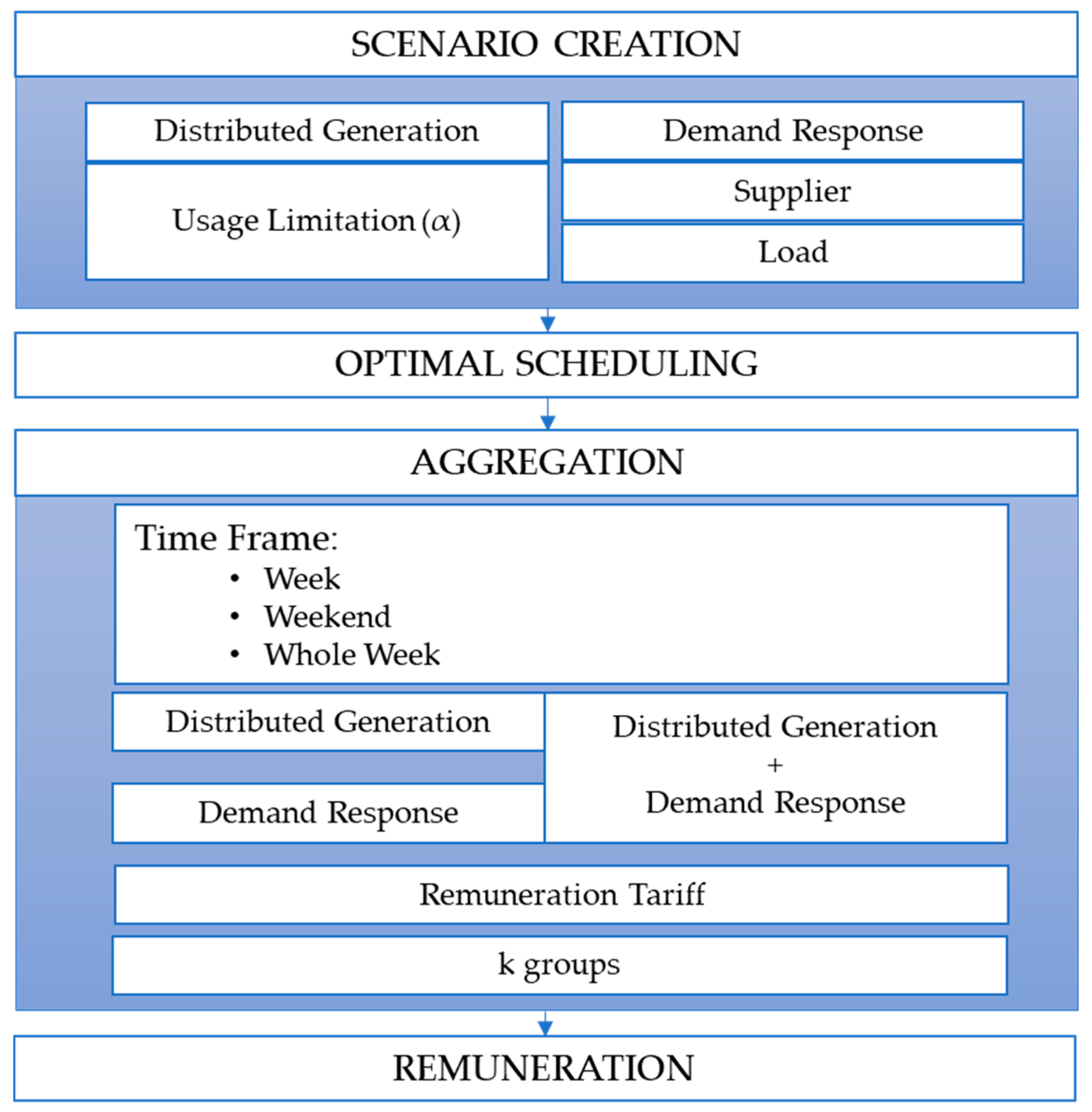
Throughout this section are presented the results obtained when applying the methodology proposed by the authors to the case study presented in the previous section. There are three sub-sections. The first one presents the results for the selected Scenario. Since there is a limitation space, the authors choose to show the full and detailed study for one scenario where k = 3. The second sub-section present the aggregated results for the remaining k scenarios studied. In the third sub-section is presented the sensitivity analysis study concerning the influence of dynamic tariffs on the remuneration of DR.

5.1. Selected Scenario: k = 3

Although the main focus is on the consumers’ results regarding DR programs, the results of the optimization for wind generation, when k = 3, are presented. The results from one wind producer for each group found through k-means are presented in Figure 7.

As can be seen, there are many periods in which the result for these three wind producers reaches a value of 0, however, when comparing with Figure 2, there was wind in these periods. This is the effect of cut-in and cut-out wind speeds.

Since the second phase of the proposed methodology is the focus of this work, one of the k values was selected, k = 3. The aggregation phase is done using the clustering method k-means through software R and considering separate clusters, i.e., each resource is grouped by type—DR and DG. Consumers of IDR programs will be the focus of this study being the only resources considered in the aggregation presented in this section. As mentioned and due to the high number of consumers in the database studied, Figure 8 shows the results of the optimization only for Medium Commerce consumers belonging to IDR.

The figures are divided by the groups that were formed by the chosen aggregation method, k-means, for the 82 elements of Medium Commerce. The x-axis represents the periods studied, with each being assigned an identification. The database is divided into 15-min periods. To form a full week, period 1 represents the hour 00 and minute 00 of the day January 2, 2018 and the last period represents hour 23 and minute 15 of day January 8, 2018.

Figure 8a presents the results for Group 1 consisting of four elements. Through the analysis of the graph, we can see these elements are the ones that obtained a lower reduction during the week, not reaching the 20 kW in any of the studied periods. Group 2, shown in Figure 8b, consisted of 13 elements, obtained reductions between 140 and 280 kW. In relation to Group 3, Figure 8c shows the results and since this group holds most of the elements, about 65. This group contains elements that managed to reduce, although they are lower values to Group 2, between approximately 35 and 110 kW. In all the figures, there are periods in which reduction was not possible, and it is also emphasized that, when there was reduction, it is maximum and equal in all periods for each consumer.

The k-means function also gives the centroid value for each group. The centroid values allow us to estimate the average value of reduced power, making it easier to assign a new resource to a given group. Figure 9 presents this value for different aggregations studied in the proposed methodology—WW, WD and W—and always for k = 3. Due to the difference in scale of some curves, there are two y-axes to be able to see those that are in the dashed line.

Although the notation of the assigned group is different, it is possible to perceive a tendency to create groups with a similar level of centroids. In other words, there is a group of consumers, where in certain periods, it achieves high reductions up to 175kW; another with medium reductions around 50 kW and the remainder with values that do not reach ~1 kW. This information allows the aggregator to allocate new resources faster to existing groups, bypassing this step and moving to pay.

Table 3. Tariffs and Final Remuneration to all scenarios, for k = 3.

	Group	WW (m.u./kW)	WD (m.u./kW)	W (m.u./kW)
k = 3	1	0.2253	0.1986	0.1986
	2	0.1986	0.1986	0.1986
	3	0.1986	0.2253	0.1986
	Group	WW (m.u.)	WD (m.u.)	W (m.u.)
	1	894,718.97	63,726.54	54,547.41
	2	138,375.46	91,023.48	53,600.60
	3	197,646.64	737,218.48	71,026.88
Total		1,230,741.07	891,968.50	179,174.89

shows the tariffs for each group and the result of the total remuneration of the different scenarios studied in the proposed methodology, for the k selected in this section.

Through the initial price of each resource, the definition of the tariff was made finding the maximum price of each group, and all elements will be paid at the highest tariff. In this way, most of the resources will benefit, since most of these will see the price of remuneration rise. The first part of Table 3 shows the final remuneration rate of each group. The total final remuneration value was calculated by the product of the contribution of each IDR consumer and the respective group rate. That is, only the resources that were scheduled, are remunerated. When comparing the remunerations, the case of separately aggregating the WD and W would be more important for the aggregator. The resources are paid at high rates and even then, it will be possible to save in relation to WW aggregation

5.2. Other Scenarios: k = 4 to k = 6

In this subsection the results for the aggregation of consumers of IDR programs and their respective remuneration by groups will be presented. The aggregation was done once again using the capabilities of the k-means clustering method and through software R. Throughout this subsection three different k, k = 4 to k = 6 are analyzed. For each of these, three different scenarios were studied, as expected in the proposed methodology: WW, WD and W.

Table 4. Results for k = 4 to k = 6 to all scenarios.

	Group	WW (n of elements)	WD (n of elements)	W (n of elements)
k = 4	1	17858	7	1390
	2	65	20232	18842
	3	2374	19	13
	4	13	52	65
k = 5	1	14	17261	65
	2	51	13	13
	3	17858	51	14423
	4	2374	2971	4436
	5	13	14	1373
k = 6	1	13	7	51
	2	3162	1398	14
	3	1374	19	13
	4	15696	52	1373
	5	51	3238	4436
	6	14	15596	14423

shows the summary of results for the application of the selected clustering method for the three scenarios studied and for k = 4 to k = 6. This table shows the element numbers for each group. Analyzing WW, in k = 4 Group 1 gathers the largest number of elements, where 51% belong to SC and 48% to DM. Still in this group are the totality of LC and ID elements. Group 2 consists only in MC elements, containing 65 of the 85 elements belonging to the database. Group 3 is constituted by DM and SC in its majority, with only 4 MC elements. Group 4 contains the remaining MC elements. Turning to k = 5, Groups 1, 2 and 5 contain only MC elements; Group 3 is the group that aggregates more elements and contains the same elements as Group 1 of k = 4; Group 4 consists in 67% DM, 33% SC and a small percentage of MC. Finally, in k = 6, Groups 1, 5 and 6 with only MC elements; Group 2 is divided in DM and SC element; Group 3 has 99.71% DM elements and 0.29% MC; Group 4 contains all elements of the LC and ID database and still 76% of the DM and 79% of the SC.

Regarding to WD, in k = 4, Groups 1,3 and 4 consist of MC elements in their entirety; Group 2 aggregates the remaining types of consumers and only 4 MC elements. In k = 5, group 1 aggregates the total LC and ID and still a large part of elements of DM and SC, this time there is no MC in this group that contains most of the elements; the MC elements are grouped into Groups 2,3 and 5; Group 4 consists of DM in 69.84%, SC in 30.02% and MC in 0.13%. Finally, at k = 6, the elements of MC form the Groups 1,3 and 4; Group 2 consists of 90.63% DM elements, the remainder are SC and MC; group 5, unlike the previous one, is constituted mostly by SC and the remaining elements are DM; the last group, contains the elements of LC, ID, DM and SC.

For the case of W, in k = 4, Group 1 consists mostly of DM elements and 4 MC consumers; Group 2 contains 9828 elements of SC, 8782 of DM and the entire LC and ID elements from database; Group 3 and Group 4 aggregate only MC elements. At k = 5, Groups 1 and 2 comprehend only MC elements; Group 3 contains the totality of SC, LC and ID also counting with some elements of DM; Group 4 contained of elements of DM only; Group 5 contains 1369 elements of DM and 4 elements of MC. Finally, at k = 6, Groups 1, 2 and 3 have elements of MC only; Group 4 contains 99.71% DM and 0.29% MC; Group 5 is comprised in its entirety by DM and Group 6 contains all the elements of SC, LC and ID and 4363 elements of DM.

In this way it is concluded that the elements of MC are quite different from each other and from the other types, being a constant the formation of groups with only these elements. Consumers of DM and SM are similar, forming, for the most part, groups with each other. Regarding LC and ID, in all cases, they belonged to the same group.

The selected clustering method, in addition to assigning the group to each element of the database, outputs the centroid of each group. Due to space constraints, it was not possible to display all values for all periods.

Table 5. Optimization results for k = 4 to k = 6.

	Group	WW		WD		W
		Min (kW)	Max (kW)	Min (kW)	Max (kW)	Min (kW)	Max (kW)
k = 4	1	0	176.3043	0	106.6657	0	50.36435
	2	0	50.36435	0.136316	0.422015	0.065409	0.371285
	3	0.642414	1.104481	0	205.5469	0	176.3043
	4	0.069013	0.33129	0	40.38773	1.064323	1.108739
k = 5	1	0	176.3043	0.160969	0.786389	1.064323	1.108739
	2	0	39.81263	0.075423	0.28143	0.065409	0.371285
	3	0.069013	0.33129	1.222448	1.425932	0	88.80277
	4	0.642414	1.104481	0	176.3043	0	176.3043
	5	0	88.80277	0	50.36435	0	39.81263
k = 6	1	0	205.5469	0.038991	0.782142	0	0.39553
	2	0	0.830448	0	40.38773	0	176.3043
	3	0	40.38773	1.041045	1.156256	0	39.81263
	4	0.078519	0.283213	0	205.5469	1.067912	1.112878
	5	0	106.6657	0	106.6657	0	88.80277
	6	1.067699	1.112632	0.075423	0.28143	0.277825	0.29400

shows the maximum and minimum values of each group for the periods of each case.

Starting with WW, in k = 4 there are two groups that not exceed 2 kW, group 3 and 4; Group 1 reaches 176.30 kW and Group 2 reaches 50.36 kW. In k = 5, some groups remain the same in relation to the previous k, namely Group 1, group 3 and 4; Group 2 this time reaches 39.81 kW and Group 5 reaches 88.80 kW. For k = 6, the groups with the lowest value are 2, 4 and 6; the remainder are in the range of 40.38 kW and 205.54 kW.

Then the case of WD, at k = 4, the group with the lowest value does not reach 1 kW, while Groups 1, 3 and 4 reach 106.67 kW, 205.55 kW and 40.39 kW, respectively. At k = 5, there are more groups around 1 kW, these being 1,2 and 3; for Groups 5 and 6, the values are higher around 50 kW and 175 kW, respectively. Finally, k = 6, Groups 2,4 and 5 find their maxima between 40 and 205 kW approximately, while the others remain with their values close to 1 kW.

Finally, in W, k = 4 formed two groups that are around 1 kW and the rest have their maximums at 50.36 kW and 176.30 kW. In k = 5, the groups with smaller values remain as k = 4; Group 3 has a maximum of 88.80 kW, Group 4 reaches 176.30 kW and Group 5 drops to 39.81 kW. For k = 6, Group 1 does not reach 0.5 kW, Group 2 is around 180 kW, Group 3 has a maximum of 39.81 kW, Group 4 is around 1 kW, Group 5 was close to reaching 89 kW and Group 6 has a minimum value of 0.28 kW and a maximum value of 0.29 kW.

Thus, it is concluded that there are three main bands: consumers with small reductions (~1 kW), consumers with medium reductions (~39 kW and 107 kW) and consumers with high reductions (above 107 kW). The analysis of the Table 5 is useful in case the VPP wants to introduce new resources or consumers to the already aggregated ones. Through the knowledge of these three types of bands and in the case of existing historical data, VPP can perceive in which group these are inserted without having to go through all the phases again.

The remuneration of the members of the groups is made taking into account the tariffs in

Table 6. Tariffs definition for k = 4 to k = 6.

	Group	WW (m.u./kWh)	WD (m.u./kWh)	W (m.u./kWh)
k = 4	1	0.2253	0.1986	0.1986
	2	0.1986	0.2253	0.1765
	3	0.1986	0.1986	0.1986
	4	0.1986	0.1986	0.1986
k = 5	1	0.1986	0.2253	0.1986
	2	0.1986	0.1986	0.1986
	3	0.2253	0.1986	0.1765
	4	0.1986	0.1986	0.1426
	5	0.1986	0.1986	0.1986
k = 6	1	0.1986	0.1986	0.1986
	2	0.1652	0.1986	0.1986
	3	0.1986	0.1986	0.1986
	4	0.2253	0.1986	0.1986
	5	0.1986	0.1652	0.1426
	6	0.1986	0.2253	0.1765

. The tariffs presented were created taking into account the value of the initial tariff of each of the elements. The authors considered that the remuneration tariff of each group would be the maximum value of each group. Thus, all elements would benefit.

As presented, the values are higher than the case if the resources were remunerated with the initial tariff. Still, it can be advantageous for the aggregator since with the implemented tariff, the actual response from one of the resources associated with this entity is more reliable, as the resources with same characteristics will be in the same group and paid at highest price, with the proposed methodology. In this way, for WW, the lowest pay price was found through k = 6, with 1,145,528.00 m.u. If we compare this value with the sum of WD and W for k = 6, we realize that this value is higher, concluding that with a greater amount of information it will be possible to find groups that are better suited to the situation. Regarding WD, the highest value was obtained in k = 4, almost reaching 900 000,00 m.u. For the W, this is the only one that the possibility of remuneration through aggregation groups, gets a lower value than the individual, in k = 6, with 228,161.48 m.u.

The higher tariff is 0.2253 m.u./kWh, found in both WW and WD. Regarding W, since that cost was not available, the higher one, and mostly used, is 0.1986 m.u./kWh. The results of remuneration for each group and for the totals are shown in

Table 7. Final Remuneration for k = 4 to k = 6.

	Group	WW (m.u.)	WD (m.u.)	W (m.u.)
k = 4	1	571,457.12	40,005.19	58,335.39
	2	197,646.64	737,215.48	71,544.33
	3	284,952.53	56,348.93	0.00
	4	138,375.46	58,392.90	106,625.16
Total		1,192,431.75	891,962.50	236,504.89
k = 5	1	369.35	450,890.69	106,625.16
	2	14,009.66	63,725.54	74,649.92
	3	942,595.87	56,454.47	97,428.59
	4	279,183.83	252,392.82	35,114.39
	5	279.69	34,567.01	57,915.39
Total		1,236,438.40	858,030.53	371,733.44
k = 6	1	138,375.46	40,005.19	66,132.37
	2	160,509.52	149,638.62	40,492.79
	3	199,488.70	56,348.93	0.00
	4	449,507.68	58,392.90	57,915.39
	5	122,586.84	145,433.09	35,123.56
	6	75,059.80	369,117.42	28,497.37
Total		1,145,528.00	818,936.15	228,161.48

.

In Table 7, although the remuneration proposed in the methodology is higher than the total in the individual remuneration case (in most cases), this difference will be important to keep resources motivated to participate in the management of the network operation. With this, VPP will be able to reduce the uncertainty associated with the participation of these resources and even attract more resources for aggregation. To prove this, another study was carried out.

For the lowest value of remuneration found in the three k clusters studied in this section (k = 6), we intend to compare this remuneration method with other methods. Thus,

Table 8. Methods for Remuneration Comparison.

Method	Type of remuneration	Details
1	Individual	Each consumer receives according to a fix tariff
2	Average	Each consumer receives according to the average of the fixed tariff for the group that belongs
3	Formula	According to the remuneration formula presented in [15] and [29]
4	Max	According to the proposed methodology

shows the definition of the methods tested and

Table 9. Remuneration Comparison.

Method	W (m.u.)	WD (m.u.)	WW (m.u.)
1	308,915.11	750,731.99	1,059,647.10
2	313,241.99	802,476.06	1,115,718.05
3	24,582.41	61,787.27	86,369.68
4	228,161.48	818,936.15	1,145,528.00

the results obtained by method for each of the study scenarios. The results of the first phase of the methodology—optimization were considered for this study. Thus, null values also considered as consumers who have not reduced their consumption, will not be considered for the application of this methods.

Method 1 proposes that each consumer should be remunerated individually. Thus, according to what has reduced in a given period, each of the consumers receives according to the tariff applied in that same period. Method 2 applies the average for the tariffs of each type of consumer. For example, for all consumers DM is calculated the average tariff and then applied to all equally. Method 3 uses the remuneration formula presented in [15] and [28] and is done individually. Method 4 is presented in the methodology proposed in this paper.

By analyzing Table 9, it’s easy to realize that Method 3 is the one that generates the lowest total remuneration, in all cases. However, compared with the other methods, it is considered that if consumers are remunerated in this way, they may not be motivated to participate with the VPP. The remaining methods have closer results. In W, the highest value is presented by Method 2 and in the remaining, WD and WW, Method 4. It is difficult to guarantee the reduction by each consumer since it is voluntary for DR programs, however it is anticipated that the greater the incentive is, the higher is the participation. In this way, according with the limits imposed for VPP to manage the market and still remunerate each consumer fairly, Method 4 becomes the more successful. However, in order to discuss even further the relevance of the proposed methodology, another comparison was performed: taking into account that the resources are paid according their availability, in other words, the provided demand reduction, in the case of the consumers.

Table 10. Remuneration Comparison.

W (m.u.)	WD (m.u.)	WW (m.u.)
379,930.58	1,097,207.44	1,477,138.02

presents the value of remuneration with this non-discriminatory approach for the three scenarios.

Comparing the values from Table 10 with the previous Table 9, has been proven that the proposed methodology can provide lower remuneration costs for the aggregator and still reward fairly every consumer for their participation.

5.3. Influence of the variations in the dynamic tariffs

Another test was carried out to analyze the influence of the formation of the tariff on the final remuneration. In this way, tests were performed for the three different time frames. The formation of the tariff for this specific case was made through two tariffs: the fixed tariff and an indexed tariff. The indexed tariff is the real-time energy price for the week selected for the previous study case (January 2, 2018 to January 8, 2018).

Table 11. Price value for each study day.

	Jan, 2	Jan, 3	Jan, 4	Jan, 5	Jan, 6	Jan, 7	Jan, 8
Tariff (m.u./kWh)	0.04089	0.04574	0.04537	0.04478	0.04590	0.04706	0.06477

shows the average values for each day of the study week. It is emphasized that this study was done only for DR consumers associated with VPP.

The objective will be to understand the influence that this new tariff will have on the final remuneration results. To assessment this method, several tests were performed varying the weight of each of the variables that form this new tariff. Figure 10 shows the results. Fix is considered to be the study for fixed tariff only; in the following cases, the first value represents the percentage of fixed tariff present in this situation and the second value the percentage of tariff indexed in the same situation. This figure also presents a line for each k studied. This line represents the final remuneration difference between the case study with the initial tariff and the remaining ones. With this, it will be possible to understand the effect of the indexed tariff on the final remuneration.

Starting from W, it is noticeable that in the case where the tariff is fixed, the highest value was found in k = 5, not reaching this value in any other case. It is also noted that the value of the difference ceases to be negative from the 50/50 case. The highest positive difference value reached in this study was 81,469.71 m.u. in k = 5 in the 10/90 case. This would be expected, since the weight of the indexed tariff is higher and this was the case that reached the highest value of remuneration, as already mentioned.

Turning to WD, in the initial case, only fixed tariff, the remuneration value formed by k = 3 and k = 4 are very similar, these being the highest values verified. Here, the difference did not reach a positive importance, being –582,548.17 m.u. the lowest value reached. The difference of values is practically linear in all cases except for k = 6 that varies a lot regarding the others.

Concerning WW, and contrary to the other studies, the final remuneration values obtained were not very different from the initial case. The most notorious differences are found in k = 6 but although do not reach the –200,000.00 m.u. value for any case study. The value of k = 3 is equal, maintaining the difference null; in k = 4 it reaches –38,309.32 m.u.; in k = 5 the value is the same for all situations, keeping a difference of –85,213.07 m.u.

Thus, it can be concluded that, by studying the weekend and the week separately, there is an influence of the notable indexed tariff on all clusters formed. In the case of the study of the whole week, the influence of this new tariff only begins to be noticed in values greater than k.

Therefore, for VPP, it is more beneficial to consider the indexed tariff in the formation of the remuneration tariff. In this study and for most cases, the higher the percentage of the indexed tariff in the formation, the lower the final remuneration was. It should be noted, however, that the value of this indexed tariff is much lower than the fixed tariff, justifying the values obtained.

When comparing with the case of the resources being remunerated individually, for W and WD it is more beneficial to opt for this new form of remuneration because the values can be twice inferior. In relation to WW, this new approach does not compensate for 96,913.33 m.u.

Regarding the selection of k, which corresponds to the number of DR programs or remuneration tariffs to be implemented and offered by the VPP to the aggregated consumers and producers, it should be decided taking into consideration the provided results. In fact, it is not intended in the proposed methodology to provide a decision on the ideal k; it is rather intended to provide the VPP the means to make that decision since in different operation scenarios, despite the costs and remunerations resulting from the application of the proposed methodology, it can be only possible to implement a certain number of tariffs or programs according to the technical and regulatory limitations.

6. Conclusions

This paper addresses a methodology proposed by the authors to assist aggregators in managing small resources. The focus was on aggregating these resources to form fair remuneration groups that can benefit the two parties involved. With this, the aggregator will benefit because it enters with a significant amount of energy in the market and these resources will be part of a more direct form in the market transactions.

Work already done in this area refers to the remuneration of these small resources by type, that is, in the case of distributed generation units, by generator primary source. Regarding resource group definition, clustering methods are chosen for a scenario and even when different scenarios are analyzed, they are made one by one. The multi-period innovative aspect of the present paper allows to create the groups that are obtained through the selected clustering method, taking into account the behavior of the aggregate resources for a larger set of operation scenarios. It should be stressed that the various phases—scheduling, aggregation, and remuneration—are included in a single methodology, implying more precise results than if analyzed one by one. Adding this to remuneration of the resources of a given group at the same price, which in the case of the paper in question is the maximum price found in that group, also results in remuneration groups generated that will be more reliable.

The study presented shows the influence that the number of clusters has on the final remuneration of resources. It was concluded that the maximum k value chosen represented the most beneficial situation for the VPP: reducing its operating costs and offering fair rates to the associated resources so that they remain motivated to participate in the management of the market. The optimum number of clusters has been calculated in order to determine the best number of DR programs to be implemented by the VPP.

Another important aspect taken from this study is the influence that the formation of the tariff also has on the final remuneration. When comparing the fixed tariff used to remunerate resources, in this case time-of-use tariffs existing in Portugal, with the new tariff formed by a fixed and an indexed part, it is perceived that the values are lower when the percentage of rate indexed is higher.

It should be noted the flexibility that this methodology presents. In the case of the remuneration tariff for each group, it will be possible for the aggregator to set the tariff for different time frames. This scheme contradicts the basic situation in which the resources of a certain type would be paid according to their availability. Thus, in this case, they will be remunerated according to what contributed to the optimal scheduling.

As a future work, the proposed methodology has room for improvement by considering: storage systems; study of the influence for a different time frame (all year, and include the seasonality effect); new approaches to consider the uncertainty; and follow the changing aspects of dynamic tariffs.

References

1. Faria, P.; Spínola, J.; Vale, Z. Distributed energy resources scheduling and aggregation in the context of demand response programs. Energies 2018, 11, 1987. [Google Scholar] [CrossRef]
2. Kirschen, D.S. Demand-side view of electricity markets. IEEE Trans. Power Syst. 2003, 18, 520–527. [Google Scholar] [CrossRef]
3. Jia, Y.; Mi, Z.; Yu, Y.; Song, Z.; Sun, C. A Bilevel Model for Optimal Bidding and Offering of Flexible Load Aggregator in Day-Ahead Energy and Reserve Markets. IEEE Access 2018, 6, 67799–67808. [Google Scholar] [CrossRef]
4. Bartusch, C.; Wallin, F.; Odlare, M.; Vassileva, I.; Wester, L. Introducing a demand-based electricity distribution tariff in the residential sector: Demand response and customer perception. Energy Policy 2011, 39, 5008–5025. [Google Scholar] [CrossRef]
5. Negash, A.I.; Kirschen, D.S. Compensation of demand response in competitive wholesale markets vs. Retail incentives. In Proceedings of the 11th International Conference on the European Energy Market (EEM14), Krakow, Poland, 28–30 May 2014; pp. 1–5. [Google Scholar]
6. Safdarian, A.; Fotuhi-Firuzabad, M.; Lehtonen, M. Integration of price-based demand response in DisCos’ short-term decision model. IEEE Trans. Smart Grid 2014, 5, 2235–2245. [Google Scholar] [CrossRef]
7. Kotsis, G.; Moschos, I.; Corchero, C.; Cruz-Zambrano, M. Demand aggregator flexibility forecast: Price incentives sensitivity assessment. In Proceedings of the 2015 12th International Conference on the European Energy Market (EEM), Lisbon, Portugal, 19–22 May 2015; pp. 1–5. [Google Scholar]
8. Macchiaroli, R.; Riemma, S.; Miranda, S.; Fera, M.; Iannone, R. Economic evaluation model for the energy Demand Response. Energy 2016, 112, 457–468. [Google Scholar]
9. Palensky, P.; Dietrich, D. Demand side management: Demand response, intelligent energy systems, and smart loads. IEEE Trans. Ind. Inform. 2011, 7, 381–388. [Google Scholar] [CrossRef]
10. Faria, P.; Spínola, J.; Vale, Z. Aggregation and Remuneration of Electricity Consumers and Producers for the Definition of Demand-Response Programs. IEEE Trans. Ind. Inform. 2016, 12, 952–961. [Google Scholar] [CrossRef]
11. Vergados, D.J.; Mamounakis, I.; Makris, P.; Varvarigos, E. Prosumer clustering into virtual microgrids for cost reduction in renewable energy trading markets. Sustain. Energy Grids Netw. 2016, 7, 90–103. [Google Scholar] [CrossRef]
12. Pei, W.; Du, Y.; Deng, W.; Sheng, K.; Xiao, H.; Qu, H. Optimal Bidding Strategy and Intramarket Mechanism of Microgrid Aggregator in Real-Time Balancing Market. IEEE Trans. Ind. Inform. 2016, 12, 587–596. [Google Scholar] [CrossRef]
13. Spinola, J.; Faia, R.; Faria, P.; Vale, Z. Clustering optimization of distributed energy resources in support of an aggregator. In Proceedings of the 2017 IEEE Symposium Series on Computational Intelligence (SSCI), Honolulu, HI, USA, 27 November–1 December 2018; pp. 1–6. [Google Scholar]
14. Celebi, M.E.; Kingravi, H.A.; Vela, P.A. A comparative study of efficient initialization methods for the k-means clustering algorithm. Expert Syst. Appl. 2013, 40, 200–210. [Google Scholar] [CrossRef] [Green Version]
15. Vaneghi, S.M.; Mashhadi, M.R.; Barazesh, M. Introducing a new approach to improve demand response pricing for industrial customers in Iran. In Proceedings of the 2015 Smart Grid Conference (SGC), Tehran, Iran, 22–23 December 2015; pp. 86–91. [Google Scholar]
16. Henriquez, R.; Wenzel, G.; Olivares, D.E.; Negrete-Pincetic, M. Participation of demand response aggregators in electricity markets: Optimal portfolio management. IEEE Trans. Smart Grid 2018, 9, 4861–4871. [Google Scholar] [CrossRef]
17. Li, Y.; Yang, Z.; Li, G.; Mu, Y.; Zhao, D.; Chen, C.; Shen, B. Optimal scheduling of isolated microgrid with an electric vehicle battery swapping station in multi-stakeholder scenarios: A bi-level programming approach via real-time pricing. Appl. Energy 2018, 232, 54–68. [Google Scholar] [CrossRef]
18. Silva, C.; Faria, P.; Vale, Z. Discussing Different Clustering Methods for the Aggregation of Demand Response and Distributed Generation. In Proceedings of the 2018 IEEE Symposium Series on Computational Intelligence (SSCI), Bangalore, India, 18–21 November 2018. [Google Scholar]
19. Sarker, M.; Ortega-Vazquez, M.; Kirschen, D. Optimal coordination and scheduling of demand response via monetary incentives. IEEE Trans. Smart Grid 2015, 6, 1341–1352. [Google Scholar] [CrossRef]
20. Chen, C.; Kishore, S.; Wang, Z.; Alizadeh, M.; Scaglione, A. How will demand response aggregators affect electricity markets? A Cournot game analysis. In Proceedings of the 2012 5th International Symposium on Communications, Control and Signal Processing, Rome, Italy, 2–4 May 2012; pp. 1–6. [Google Scholar]
21. Zhang, K.; Song, Y.; Yan, Z.; Yu, Y. Research on bidirectional decision-making for load aggregators participating in market transactions and load dispatching. Cired Open Access Proc. J. 2017, 2017, 2874–2878. [Google Scholar] [CrossRef]
22. Othman, M.M.; Hegazy, Y.G.; Abdelaziz, A.Y. Electrical energy management in unbalanced distribution networks using virtual power plant concept. Electr. Power Syst. Res. 2017, 145, 157–165. [Google Scholar] [CrossRef]
23. Riaz, S.; Marzooghi, H.; Verbic, G.; Chapman, A.C.; Hill, D.J. Generic Demand Model Considering the Impact of Prosumers for Future Grid Scenario Analysis. IEEE Trans. Smart Grid 2019, 10, 819–829. [Google Scholar] [CrossRef] [Green Version]
24. Silva, C.; Faria, P.; Vale, Z. Clustering Support for an Aggregator in a Smart Grid Context. In International Conference on Hybrid Intelligent Systems; Springer: Cham, Switzerland, 2018. [Google Scholar]
25. Silva, C.; Faria, P.; Vale, Z. Assessment of Distributed Generation Units Remuneration Using Different Clustering Methods for Aggregation. In Proceedings of the 2018 IEEE International Conference on Communications, Control, and Computing Technologies for Smart Grids (SmartGridComm), Aalborg, Denmark, 29–31 October 2018. [Google Scholar]
26. RWE Npower Renewables. Wind Turbine Power Calculations RWE npower renewables Mechanical and Electrical Engineering. R. Acad. Eng. 2007. Available online: https://www.raeng.org.uk/publications/other/23-wind-turbine (accessed on 30 March 2019).
27. Purnima, B.; Arvind, K. EBK-Means: A Clustering Technique based on Elbow Method and K-Means in WSN. Int. J. Comput. Appl. 2014, 105, 17–24. [Google Scholar]
28. Lletí, R.; Ortiz, M.C.; Sarabia, L.A.; Sánchez, M.S. Selecting variables for k-means cluster analysis by using a genetic algorithm that optimises the silhouettes. Anal. Chim. Acta 2004, 515, 87–100. [Google Scholar] [CrossRef]
29. Cabrera, N.G.; Gutierrez-Alcaraz, G. Evaluating demand response programs based on demand management contracts. In Proceedings of the 2012 IEEE Power and Energy Society General Meeting, San Diego, CA, USA, 22–26 July 2012; pp. 1–6. [Google Scholar]
Figure 1. Overall definition of proposed methodology.
Energies 12 01248 g001
Figure 2. Wind speed.
Energies 12 01248 g002
Figure 3. Cut-in and cut-out speed.
Energies 12 01248 g003
Figure 4. Different scenarios formed for the case study.
Energies 12 01248 g004
Figure 5. Elbow method results.
Energies 12 01248 g005
Figure 6. Silhouette method results.
Energies 12 01248 g006
Figure 7. Optimization results for three wind producers.
Energies 12 01248 g007
Figure 8. Results of the optimization for Medium Commerce consumers belonging to IDR.
Energies 12 01248 g008
Figure 9. Comparison between different scenarios, for k = 3.
Energies 12 01248 g009
Figure 10. Results for the study of the influence of the tariff in the final remuneration.
Energies 12 01248 g010