Optimal Design of Wireless Charging Electric Bus System Based on Reinforcement Learning


Abstract
:
1. Introduction
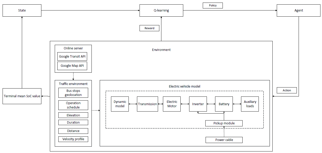
- We propose a precise model of a wireless charging electric bus system based on a Markov decision process (MDP), which is composed of environment, state, action, reward, and policy.
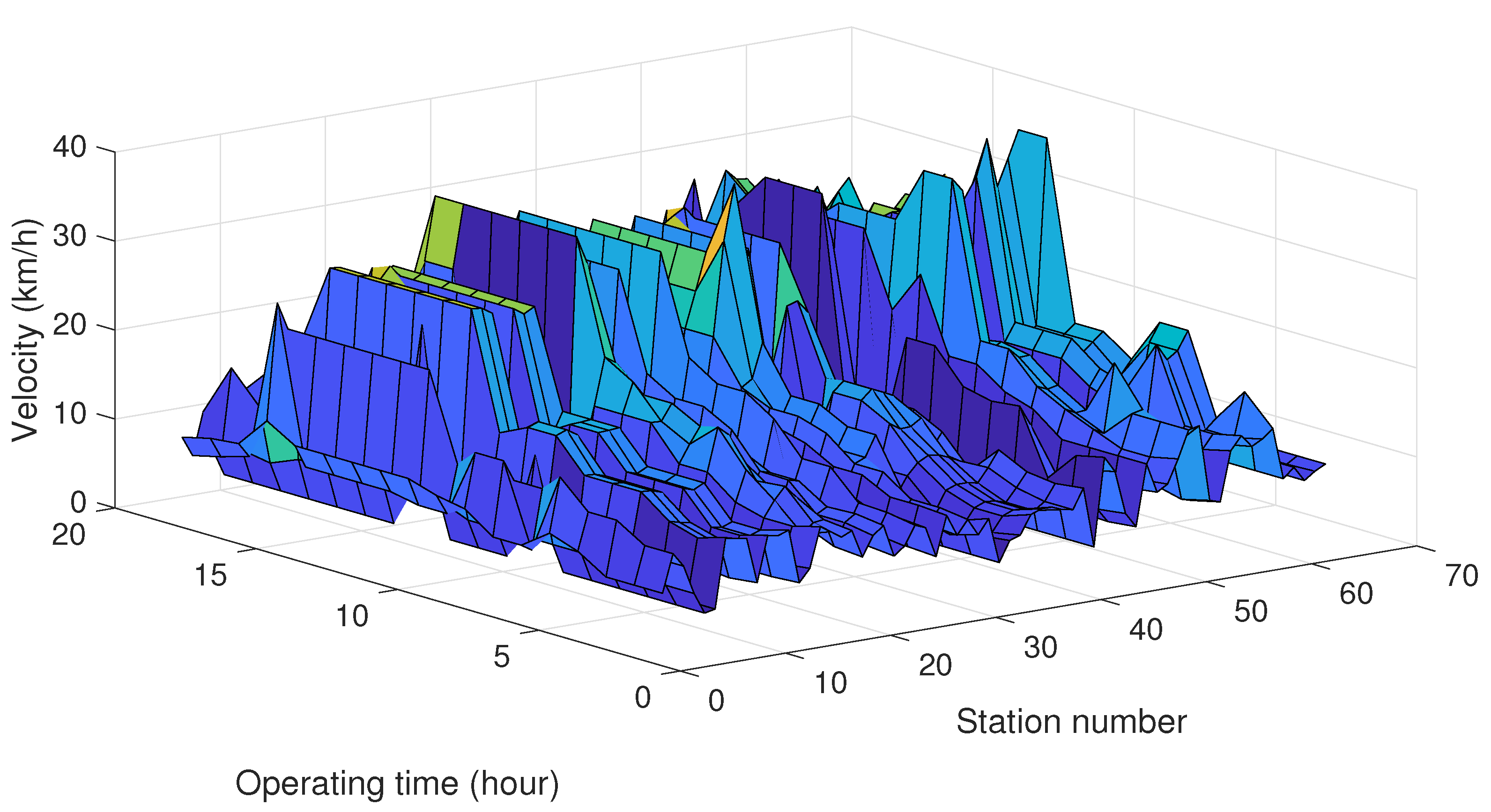
- For accurate analysis, Google Transit API and Google Map API were used to build the velocity profile of a bus fleet operating on the NYC Metropolitan Transportation Authority (MTA) M1 route. The velocity profile varies depending on operation time, which results in a more realistic optimal result.
- The suboptimal design of a wireless charging electric bus system based on reinforcement learning was modeled to find the optimal values of battery capacity, pickup capacity, and the number of power-cable installations.
- A simulation of the proposed model was conducted for both static and dynamic traffic environments.
2. Modeling of Wireless Charging Electric Bus System
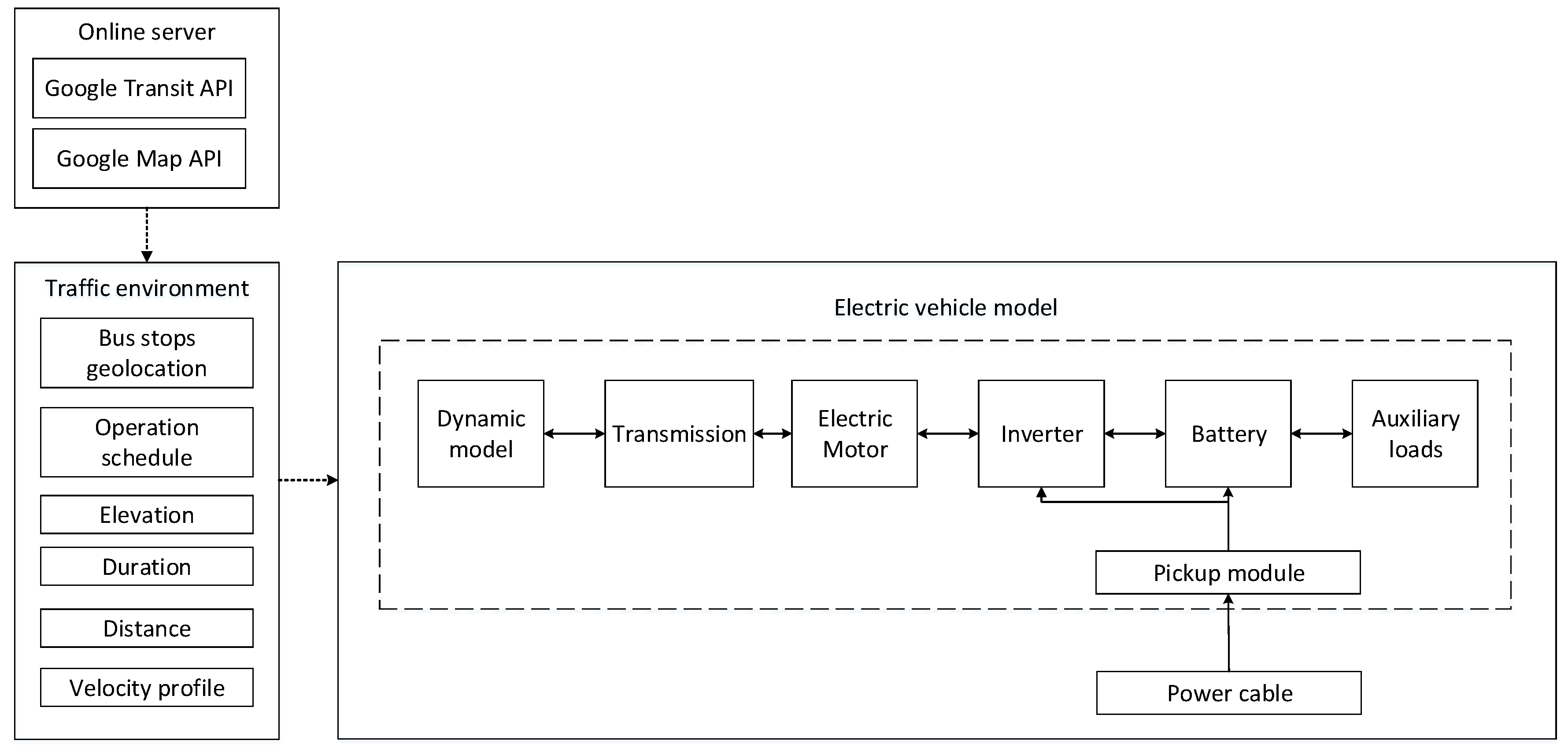
2.1. Environment
- Geolocation information (latitude and longitude) for all 64 stops was found.
- Departure and arrival times were found for neighboring stations. Mean velocity was calculated using time differences and distances between all 64 stations.
- Velocity profile was constructed using mean velocity, deceleration, and acceleration data for the electric bus.
2.2. System Modeling
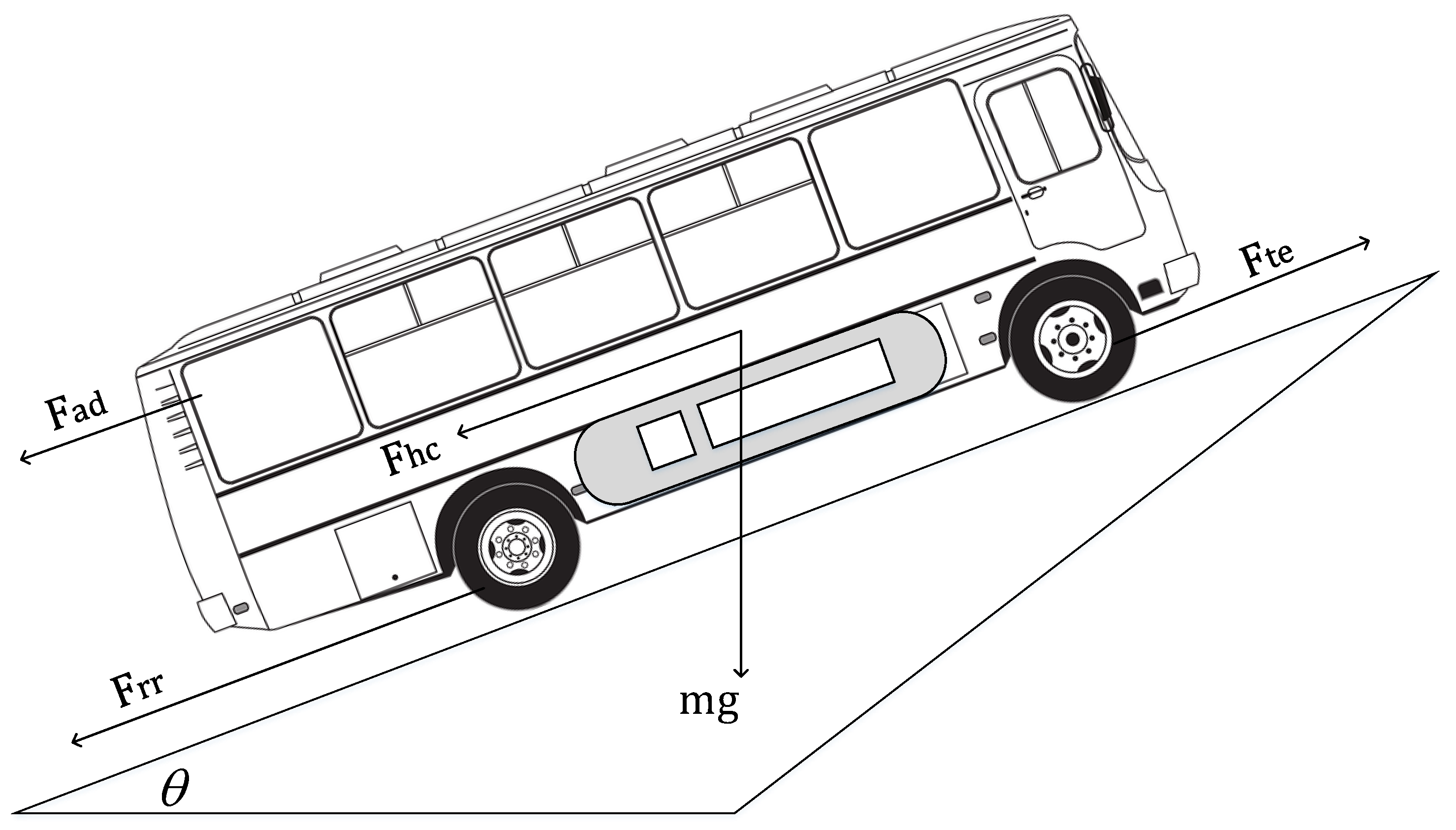
2.2.1. Dynamic Characteristics of Wireless Charging Electric Bus
2.2.2. Transmission
2.2.3. Electric Motor
2.2.4. Inverter
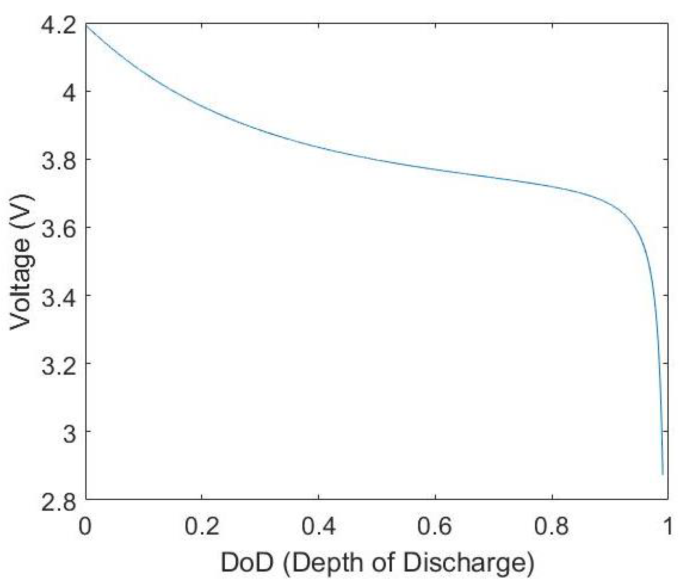
2.2.5. Battery
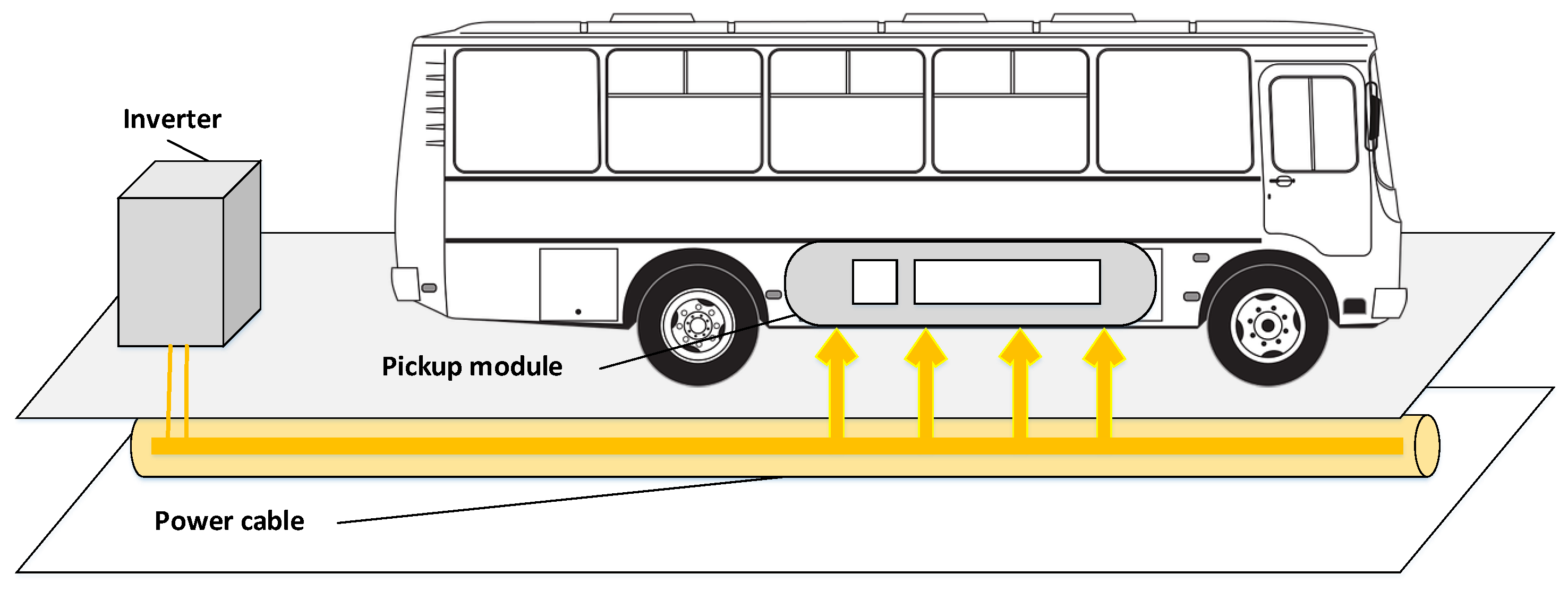
2.2.6. Wireless Charging Module
3. Suboptimal Design of Wireless Charging Electric Bus System Based on Reinforcement Learning
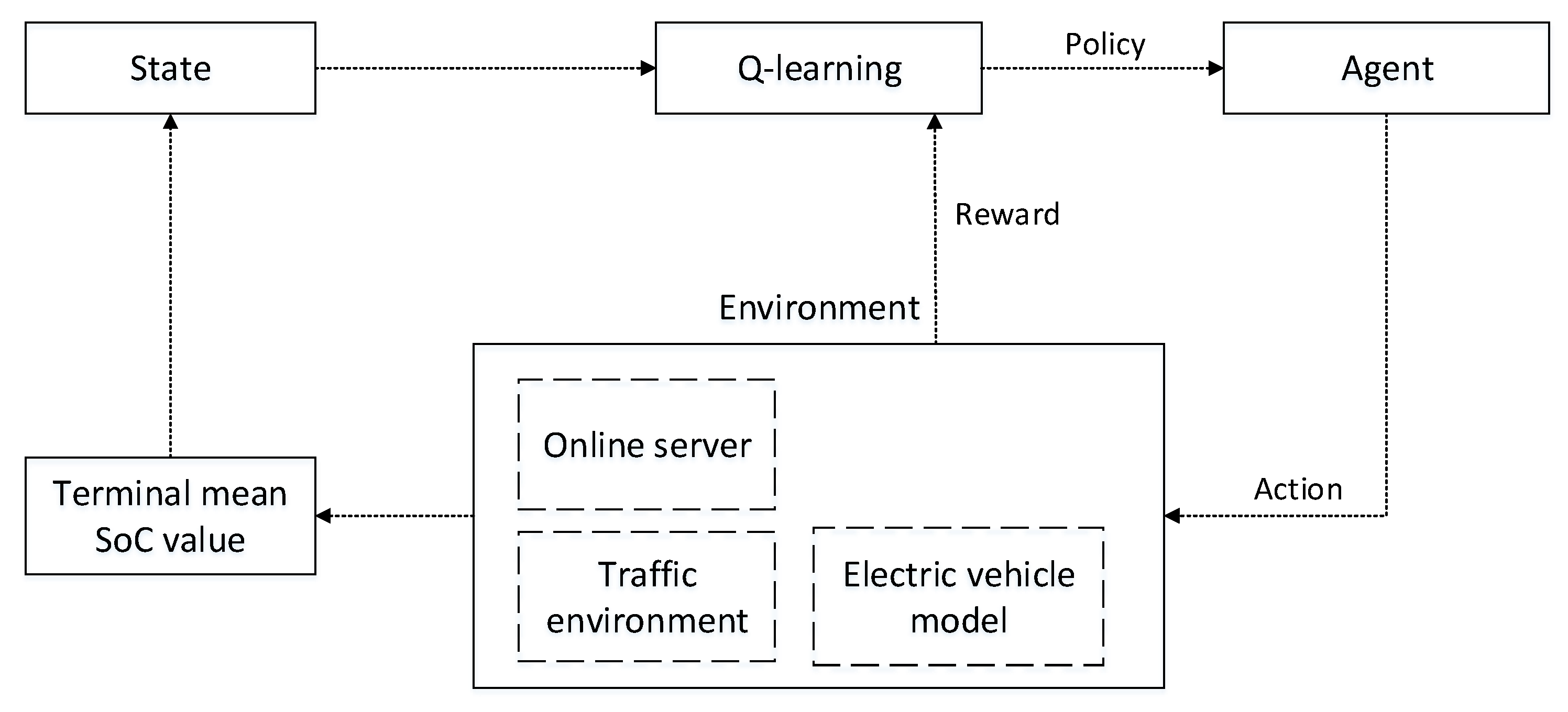
3.1. Action-State Value Update
- During Q-learning, any increase or decrease in each variable can easily be checked.
- Each dimension links to each action: the change of battery capacity, pickup capacity, and power-cable installation number.
- The agent only needs to search the actions around the current state, not the whole Q table.
- After random sampling, exploitation converges much faster because each Q-value has its own unique domain.
| Algorithm 1 Proposed optimization algorithm |
 |
3.2. State
3.3. Action and Reward
4. Results and Discussion
4.1. Simulation Environment
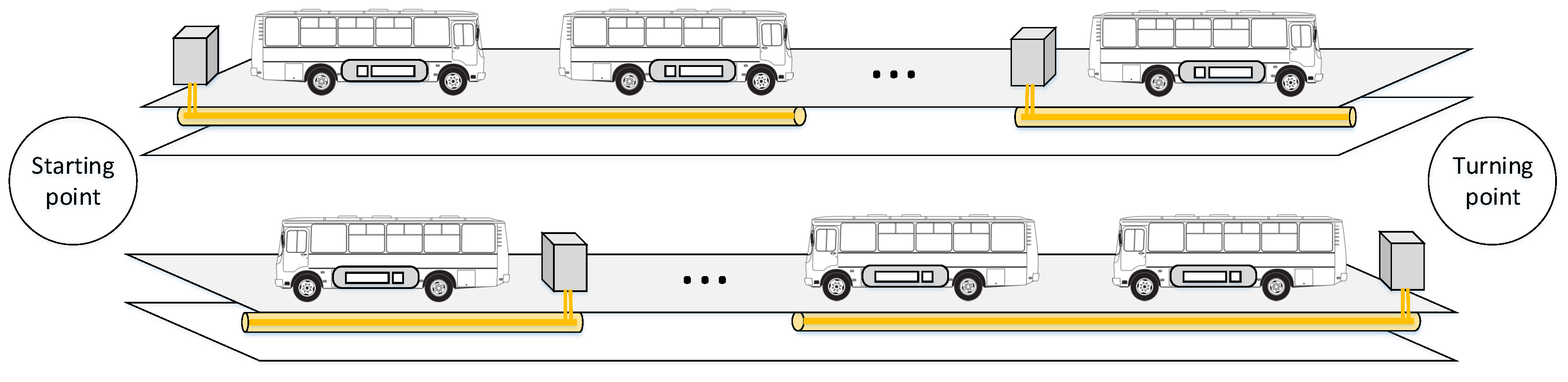
- Simulation begins when dynamic charging electric buses move forward from their starting points.
- Each electric bus departs with a fully charged battery and stops at each station for 20 to 40 s.
- The number of passengers boarding the bus differs over the timeline, and this, in turn, affects the total weight of the bus. The number of passengers peaks during commuting time and gradually reduces.
- The velocity-profile changes and the data for each episode are directly obtained from Google Map API.
- The route length is fixed, and the journey ends when the wireless charging electric bus returns to its starting point.
- The bus receives power from a single source, namely, the power cables installed underground.
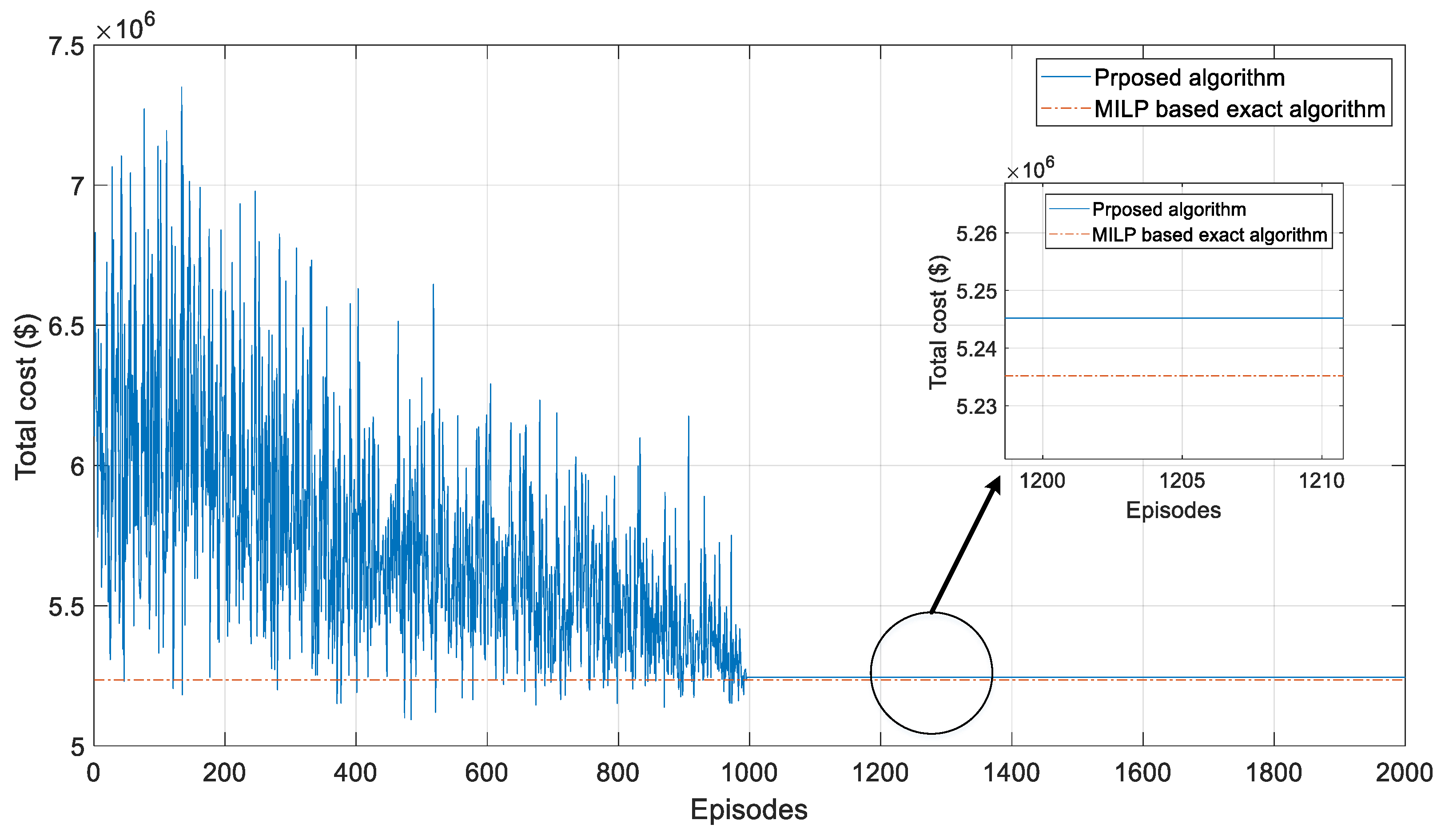
4.2. MIP-Based Exact Algorithm
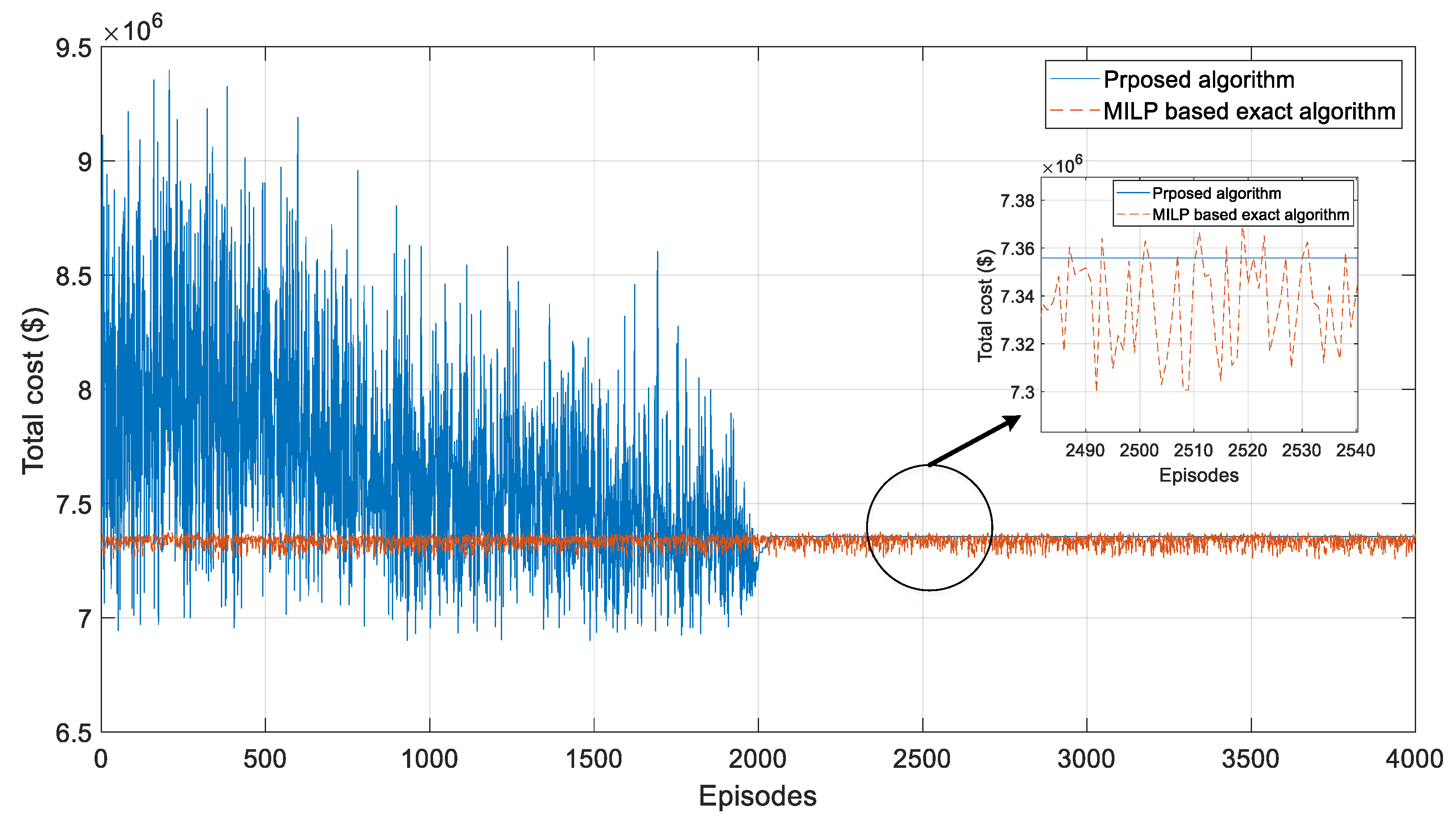
4.3. Convergence of Proposed Optimization Algorithm
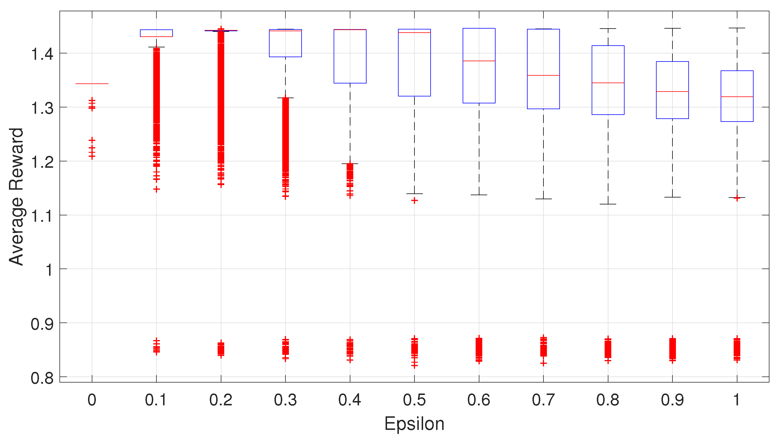
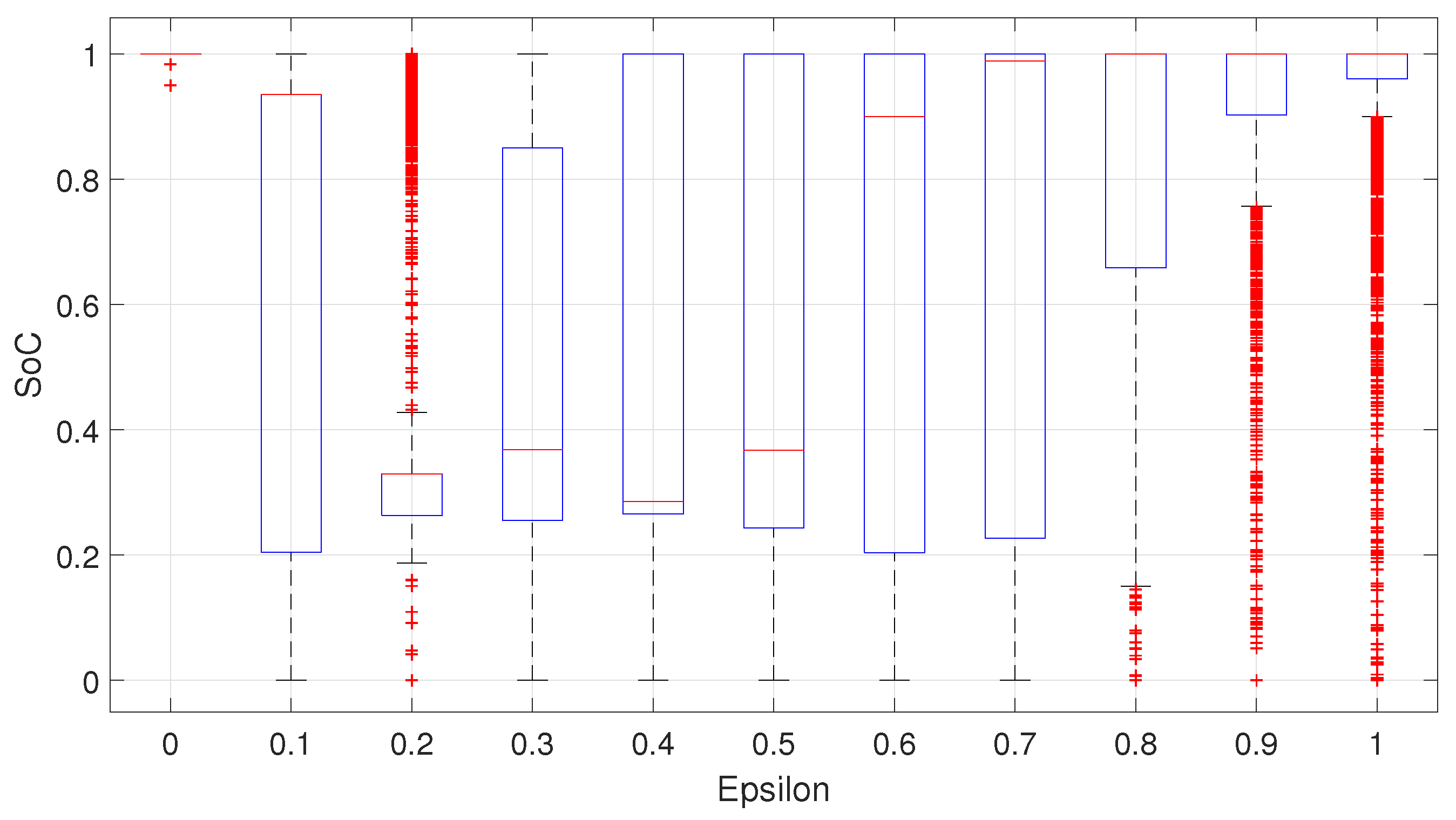
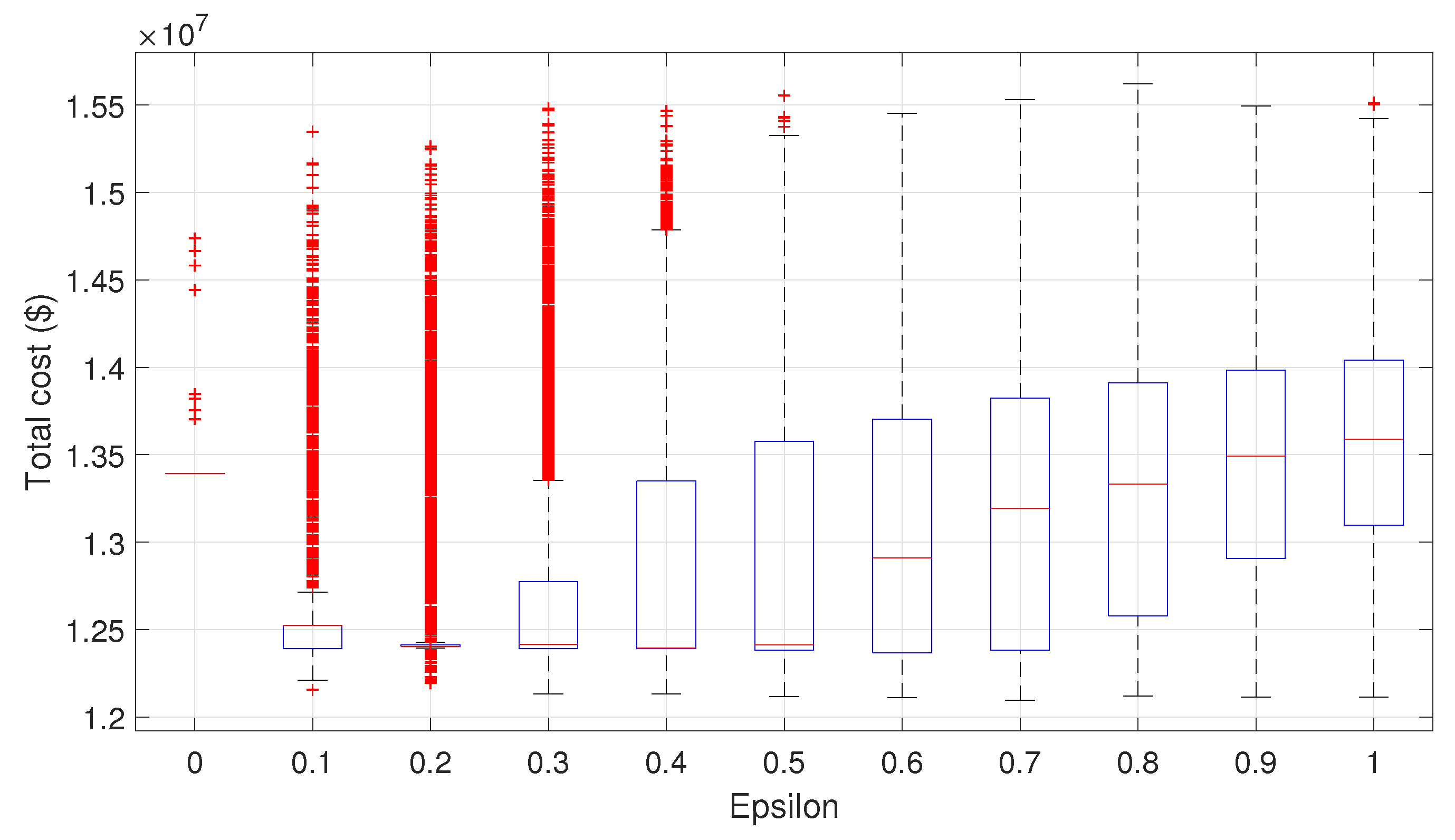
4.4. Analysis in a Static Traffic Environment
4.5. Analysis in a Dynamic Traffic Environment
5. Conclusions
Author Contributions
Funding
Conflicts of Interest
References
- Suh, N.P.; Cho, D.H. Making the Move: From Internal Combustion Engines to Wireless Electric Vehicles. In The On-line Electric Vehicle; Springer: Cham, Switzerland, 2017; pp. 3–15. [Google Scholar]
- Kan, T.; Nguyen, T.D.; White, J.C.; Malhan, R.K.; Mi, C.C. A new integration method for an electric vehicle wireless charging system using LCC compensation topology: Analysis and design. IEEE Trans. Power Electron. 2017, 32, 1638–1650. [Google Scholar] [CrossRef]
- Bi, Z.; Kan, T.; Mi, C.C.; Zhang, Y.; Zhao, Z.; Keoleian, G.A. A review of wireless power transfer for electric vehicles: Prospects to enhance sustainable mobility. Appl. Energy 2016, 179, 413–425. [Google Scholar] [CrossRef]
- Li, S.; Liu, Z.; Zhao, H.; Zhu, L.; Shuai, C.; Chen, Z. Wireless power transfer by electric field resonance and its application in dynamic charging. IEEE Trans. Ind. Electron. 2016, 63, 6602–6612. [Google Scholar] [CrossRef]
- Tan, L.; Guo, J.; Huang, X.; Liu, H.; Yan, C.; Wang, W. Power Control Strategies of On-Road Charging for Electric Vehicles. Energies 2016, 9, 531. [Google Scholar] [CrossRef]
- Kim, H.; Song, C.; Kim, D.H.; Jung, D.H.; Kim, I.M.; Kim, Y.I.; Kim, J. Coil design and measurements of automotive magnetic resonant wireless charging system for high-efficiency and low magnetic field leakage. IEEE Trans. Microw. Theory Tech. 2016, 64, 383–400. [Google Scholar] [CrossRef]
- Suh, N.P.; Cho, D.H. The On-Line Electric Vehicle: Wireless Electric Ground Transportation Systems; Springer: Cham, Switzerland, 2017; pp. 20–24. [Google Scholar]
- Mi, C.C.; Buja, G.; Choi, S.Y.; Rim, C.T. Modern advances in wireless power transfer systems for roadway powered electric vehicles. IEEE Trans. Ind. Electron. 2016, 63, 6533–6545. [Google Scholar] [CrossRef]
- Manshadi, S.D.; Khodayar, M.E.; Abdelghany, K.; Üster, H. Wireless charging of electric vehicles in electricity and transportation networks. IEEE Trans. Smart Grid 2018, 9, 4503–4512. [Google Scholar] [CrossRef]
- Bi, Z.; Keoleian, G.A.; Ersal, T. Wireless charger deployment for an electric bus network: A multi-objective life cycle optimization. Appl. Energy 2018, 225, 1090–1101. [Google Scholar] [CrossRef]
- Jang, Y.J.; Jeong, S.; Lee, M.S. Initial energy logistics cost analysis for stationary, quasi-dynamic, and dynamic wireless charging public transportation systems. Energies 2016, 9, 483. [Google Scholar] [CrossRef]
- Chokkalingam, B.; Padmanaban, S.; Siano, P.; Krishnamoorthy, R.; Selvaraj, R. Real-time forecasting of EV charging station scheduling for smart energy systems. Energies 2017, 10, 377. [Google Scholar] [CrossRef]
- Luo, Y.; Zhu, T.; Wan, S.; Zhang, S.; Li, K. Optimal charging scheduling for large-scale EV (electric vehicle) deployment based on the interaction of the smart-grid and intelligent-transport systems. Energy 2016, 97, 359–368. [Google Scholar] [CrossRef]
- Javaid, N.; Javaid, S.; Abdul, W.; Ahmed, I.; Almogren, A.; Alamri, A.; Niaz, I.A. A hybrid genetic wind driven heuristic optimization algorithm for demand side management in smart grid. Energies 2017, 10, 319. [Google Scholar] [CrossRef]
- Deilami, S. Online coordination of plug-in electric vehicles considering grid congestion and smart grid power quality. Energies 2018, 11, 2187. [Google Scholar] [CrossRef]
- Khan, S.U.; Mehmood, K.K.; Haider, Z.M.; Bukhari, S.B.A.; Lee, S.J.; Rafique, M.K.; Kim, C.H. Energy Management Scheme for an EV Smart Charger V2G/G2V Application with an EV Power Allocation Technique and Voltage Regulation. Appl. Sci. 2018, 8, 648. [Google Scholar] [CrossRef]
- Alhazmi, Y.A.; Mostafa, H.A.; Salama, M.M. Optimal allocation for electric vehicle charging stations using Trip Success Ratio. Int. J. Electr. Power Energy Syst. 2017, 91, 101–116. [Google Scholar] [CrossRef]
- Doan, V.D.; Fujimoto, H.; Koseki, T.; Yasuda, T.; Kishi, H.; Fujita, T. Allocation of Wireless Power Transfer System From Viewpoint of Optimal Control Problem for Autonomous Driving Electric Vehicles. IEEE Trans. Intell. Transp. Syst. 2017, 19, 3255–3270. [Google Scholar] [CrossRef]
- Chopra, S.; Bauer, P. Driving range extension of EV with on-road contactless power transfer—A case study. IEEE Trans. Ind. Electron. 2013, 60, 329–338. [Google Scholar] [CrossRef]
- Van Vreckem, B.; Borodin, D.; De Bruyn, W.; Nowé, A. A Reinforcement Learning Approach to Solving Hybrid Flexible Flowline Scheduling Problems. In Proceedings of the 6th Multidisciplinary International Conference on Scheduling: Theory and Applications (MISTA), Gent, Belgium, 27–29 August 2013. [Google Scholar]
- New York City MTA. Available online: http://www.mta.info/ (accessed on 5 January 2019).
- Mesbahi, T.; Khenfri, F.; Rizoug, N.; Chaaban, K.; Bartholomeues, P.; Le Moigne, P. Dynamical modeling of Li-ion batteries for electric vehicle applications based on hybrid Particle Swarm–Nelder–Mead (PSO–NM) optimization algorithm. Electr. Power Syst. Res. 2016, 131, 195–204. [Google Scholar] [CrossRef]
- Williamson, S.S.; Emadi, A.; Rajashekara, K. Comprehensive efficiency modeling of electric traction motor drives for hybrid electric vehicle propulsion applications. IEEE Trans. Veh. Technol. 2007, 56, 1561–1572. [Google Scholar] [CrossRef]
- Ahn, K.; Bayrak, A.E.; Papalambros, P.Y. Electric vehicle design optimization: Integration of a high-fidelity interior-permanent-magnet motor model. IEEE Trans. Veh. Technol. 2015, 64, 3870–3877. [Google Scholar] [CrossRef]
- Gong, X.; Xiong, R.; Mi, C.C. A data-driven bias-correction-method-based lithium-ion battery modeling approach for electric vehicle applications. IEEE Trans. Ind. Appl. 2016, 52, 1759–1765. [Google Scholar]
- Tremblay, O.; Dessaint, L.A.; Dekkiche, A.I. A generic battery model for the dynamic simulation of hybrid electric vehicles. In Proceedings of the IEEE Vehicle Power and Propulsion Conference, Arlington, TX, USA, 9–12 September 2007. [Google Scholar]
- Zhang, W.; White, J.C.; Abraham, A.M.; Mi, C.C. Loosely coupled transformer structure and interoperability study for EV wireless charging systems. IEEE Trans. Power Electron. 2015, 30, 6356–6367. [Google Scholar] [CrossRef]
- Li, S.; Mi, C.C. Wireless power transfer for electric vehicle applications. IEEE J. Emerg. Sel. Top. Power Electron. 2015, 3, 4–17. [Google Scholar]
- Mnih, V.; Kavukcuoglu, K.; Silver, D.; Rusu, A.A.; Veness, J.; Bellemare, M.G.; Petersen, S. Human-level control through deep reinforcement learning. Nature 2015, 518, 529. [Google Scholar] [CrossRef]
- Wei, Q.; Lewis, F.L.; Sun, Q.; Yan, P.; Song, R. Discrete-time deterministic Q-learning: A novel convergence analysis. IEEE Trans. Cybern. 2017, 47, 1224–1237. [Google Scholar] [CrossRef]


| Parameters | Value |
|---|---|
| Polarization voltage (V), K | 0.00876 |
| Battery constant voltage (V), | 3.7348 |
| Battery capacity (Ah), | 6.2 |
| Exponential zone amplitude, A | 0.468 |
| Exponential zone time constant inverse Ah, B | 3.5294 |
| Temperature Celsius, T | 25 |
| Parameters | Cost ($) |
|---|---|
| Price of battery capacity ($/kWh), | 290 |
| Price of inverter capacity ($/kW), | 120 |
| Price of power cable segment ($/No.), | 5000 |
| Price of electric bus ($/No.), | 160,000 |
| Route length (km) | 20.2 |
| Variables | Static Traffic Environment | Dynamic Traffic Environment |
|---|---|---|
| Number of operating buses | 25 | 34 |
| Battery capacity | 24 kWh | 29 kWh |
| Pickup capacity | 77 kW | 138 kW |
| Number of installed power-cable segments | 5 | 12 |
© 2019 by the authors. Licensee MDPI, Basel, Switzerland. This article is an open access article distributed under the terms and conditions of the Creative Commons Attribution (CC BY) license (http://creativecommons.org/licenses/by/4.0/).
Share and Cite
Lee, H.; Ji, D.; Cho, D.-H. Optimal Design of Wireless Charging Electric Bus System Based on Reinforcement Learning. Energies 2019, 12, 1229. https://doi.org/10.3390/en12071229
Lee H, Ji D, Cho D-H. Optimal Design of Wireless Charging Electric Bus System Based on Reinforcement Learning. Energies. 2019; 12(7):1229. https://doi.org/10.3390/en12071229
Chicago/Turabian StyleLee, Hyukjoon, Dongjin Ji, and Dong-Ho Cho. 2019. "Optimal Design of Wireless Charging Electric Bus System Based on Reinforcement Learning" Energies 12, no. 7: 1229. https://doi.org/10.3390/en12071229