Optimal Placement of UHF Sensors for Accurate Localization of Partial Discharge Source in GIS

Abstract

This paper proposes an optimal placement model of ultra-high frequency (UHF) sensors for accurate location of partial discharge (PD) in gas-insulated switchgear (GIS). The model is based on 0-1 program in consideration of the attenuation influence on the propagation of electromagnetic (EM) waves generated by PD in GIS. the optimal placement plan improves the economy, observability, and accuracy of PD locating. After synchronously acquiring the time of the initial EM waves reaching each UHF sensor, PD occurring time can be obtained. Then, initial locating results can be acquired by using the Euclidean distance measuring method and the extended time difference of arriving (TDOA) location method. With the information of all UHF sensors and the inherent topological structure of GIS, the locating accuracy can be further improved. The method is verified by experiment, showing that the method can avoid the influence of false information and obtain higher locating accuracy by revising initial locating results.

1. Introduction

With the wide use of gas-insulated switchgear (GIS), various failures occur with the growth of service time, and the insulation defects in GIS may lead to partial discharge (PD). PD location can be realized via ultrasonic waves and ultra-high frequency (UHF) electromagnetic (EM) waves [1,2,3]. The UHF method is an efficient PD detection technology that detects the EM wave generated by PD based on UHF sensors [4,5,6,7,8]. The UHF method has the advantages of high sensitivity and high signal-to-noise ratio. The position of PD can be located by analyzing and processing the EM signal received by the sensors [9,10,11]. UHF location methods are mainly based on time difference of arriving, time of arriving, angle of arriving, and received signal strength [12,13].

The spatial placement of UHF sensors is the key to PD locating. Studies have been undertaken to improve sensor economy and observability. Though some exploratory research works have been carried out in these fields, most of them focused on transformer or conventional switchgear [14,15,16,17,18]. For instance, a spatial array of UHF sensors is used for transformer PD location. However, a transformer is a multisurface system of which the internal structure is totally different from GIS. The spatial array aims to overcome the reflection and diffraction of electromagnetic waves. Therefore, the methods for transformers and switchgear are not suitable for GIS. The topological structures of GIS and the attenuation of the EM wave especially propagating through the insulators and L-type and T-type structures should be considered more. A few studies have investigated the topological structures of GIS but these do not consider the optimal placement of sensors [19,20,21,22,23]. The arriving time difference of EM waves was used to locate the PD in GIS based on UHF sensors, but its accuracy should be improved [24,25,26]. This paper is devoted to solving these problems in existing research.

In this paper, the GIS space structure is abstracted into an undirected graph and a 0-1 programming model is established based on the optimization of the optimal economy and the maximum observability. Then, an arrangement plan of UHF sensors can be obtained. With the optimal placement plan, the accurate location method of PD based on extended time difference of arriving (TDOA) is studied. The experimental result indicates that the proposed method can improve the location accuracy and possesses fine fault tolerance.

2. Principle of Method

2.1. Partial Discharge in GIS

GIS, which includes a circuit breaker, disconnector, grounding switch, transformer, and bus, has been widely used due to its low maintenance, high reliability, and compact size. PD refers to the discharge phenomenon occurring in the partial area of the insulator which does not penetrate the conductor under voltage. Under a strong electric field, the insulation defects of GIS will lead to PD, accompanied by the generation of electricity, light, heat, sound, ozone, and nitric oxide, which will corrode the insulating materials. In addition, the charged particles produced by PD will impact the insulating materials. PD is a sign of insulation degradation in GIS, which endangers the safety of equipment and even the power system.

The breakdown field strength of insulators in power equipment is very high. When PD occurs in a small range, the breakdown process is very fast, which produces steep pulse current. Its rising time is less than 1 ns, and ultra-high frequency (UHF) electromagnetic waves are excited. The principle of the UHF method for PD detection is to detect the UHF electromagnetic waves (300 MHz‒3 GHz) generated by PD in power equipment by UHF sensor. Then, the information of PD can be obtained. Built-in UHF sensors and external UHF sensors are usually used for UHF methods.

Because corona interference is mainly concentrated below the 300 MHz frequency band, the UHF method can effectively avoid corona interference. It has high sensitivity and anti-interference ability. Naturally, the optimal placement of UHF sensors and location method become the key to partial discharge locating.

2.2. Optimal Placement of UHF Sensors

The optimal placement of UHF sensors should satisfy the economy of scale and provide maximum observability. A necessary requirement for successful locating is that at least two sensors detect an effective discharge EM wave, and the EM wave must pass through both ends of the discharge section. If the EM wave only passes through the head or the end of the detecting section, the locating will fail. 1 represents that the sensor needs to be installed and 0 represents the sensor doesn’t need to be installed. Therefore, the placement of UHF sensors can be abstracted as a 0-1 programming model.

The EM wave will be attenuated when passing through the insulators and L-type and T-type structures in GIS. The vertical branches of L-type structures and T-type structures significantly attenuate the EM wave, and the attenuation caused by the horizontal branches of T-type structures and insulators comes after. In order to improve the detection sensitivity and locating reliability, the L-type structures and the T-type structures in GIS should be taken into consideration.

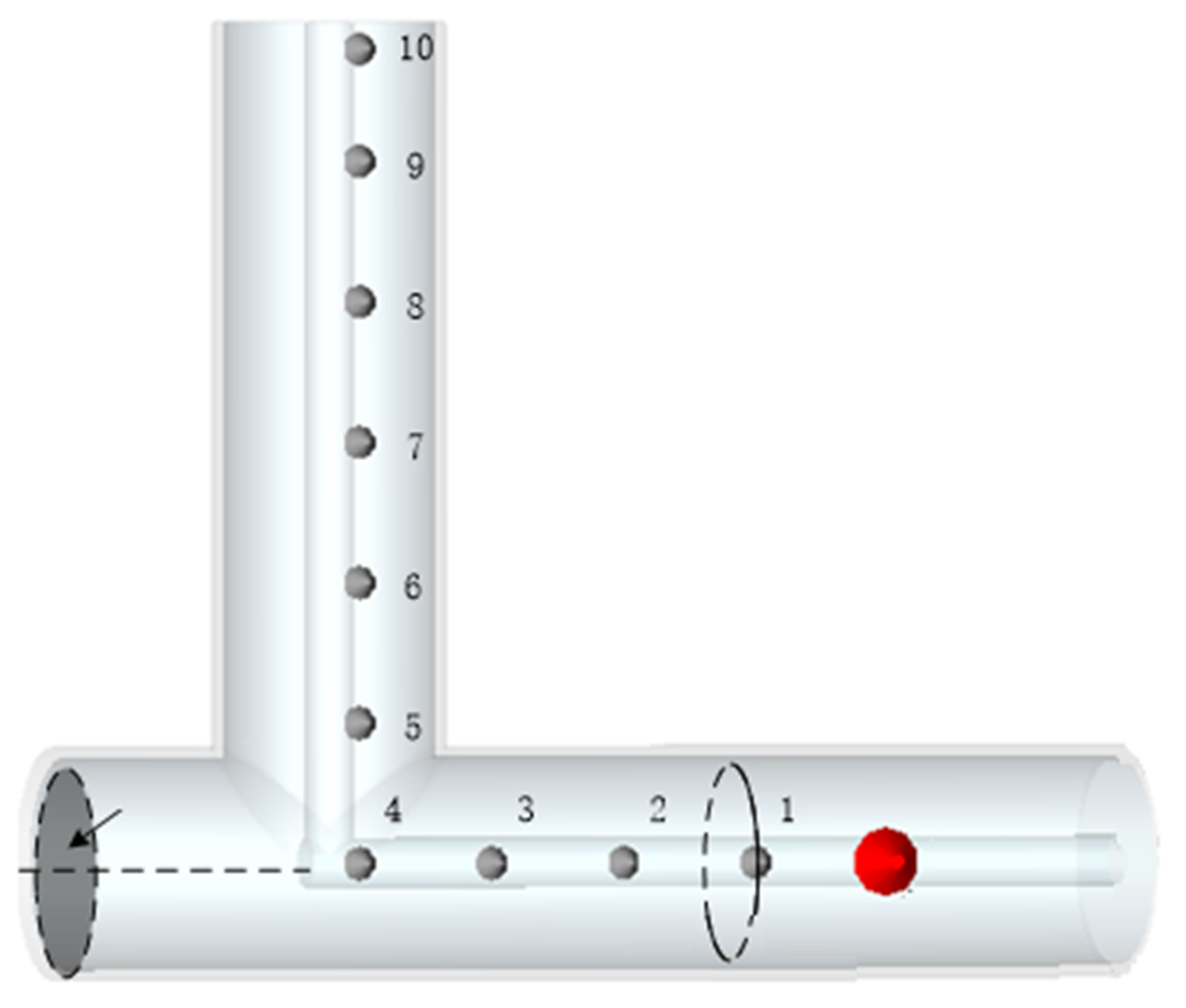
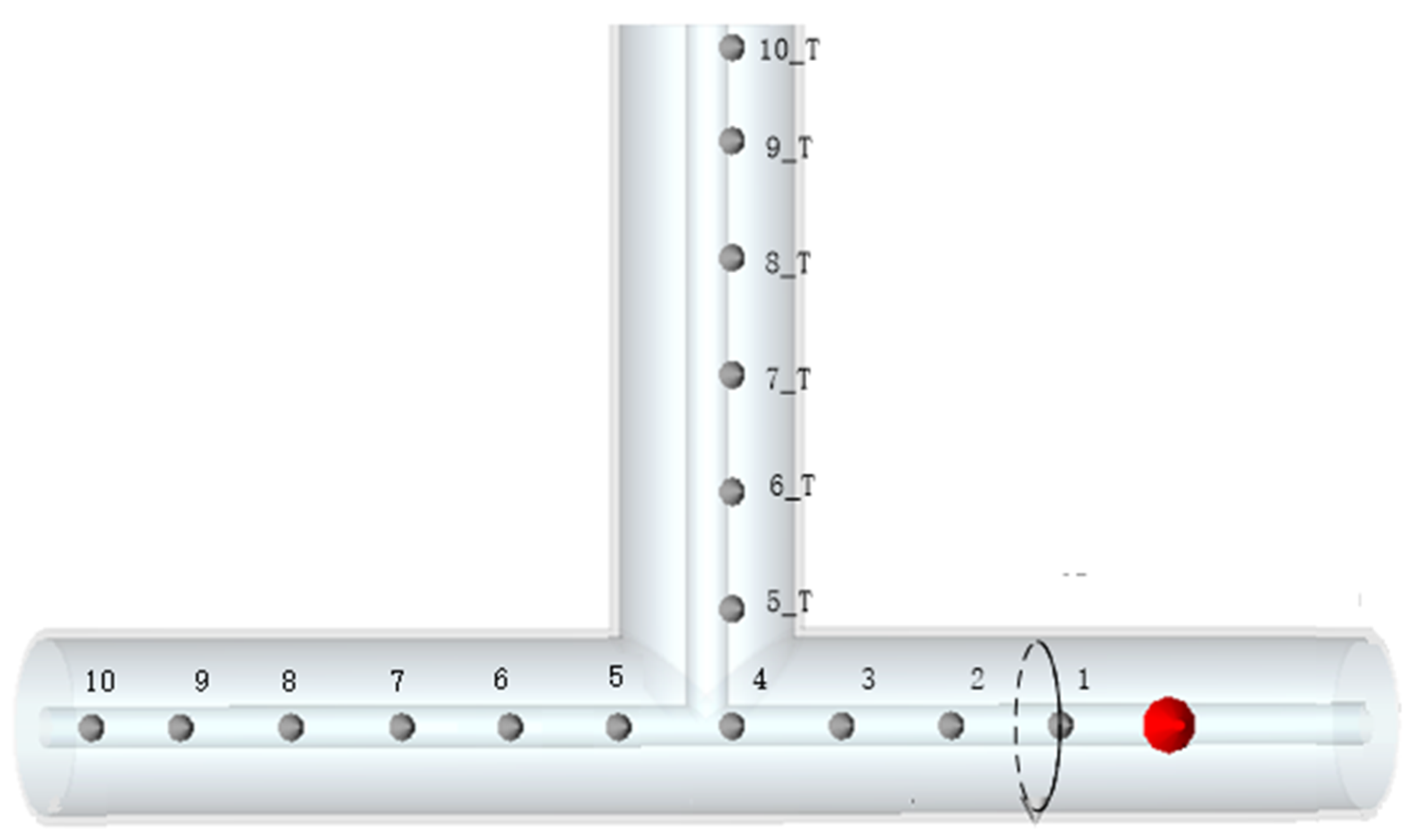
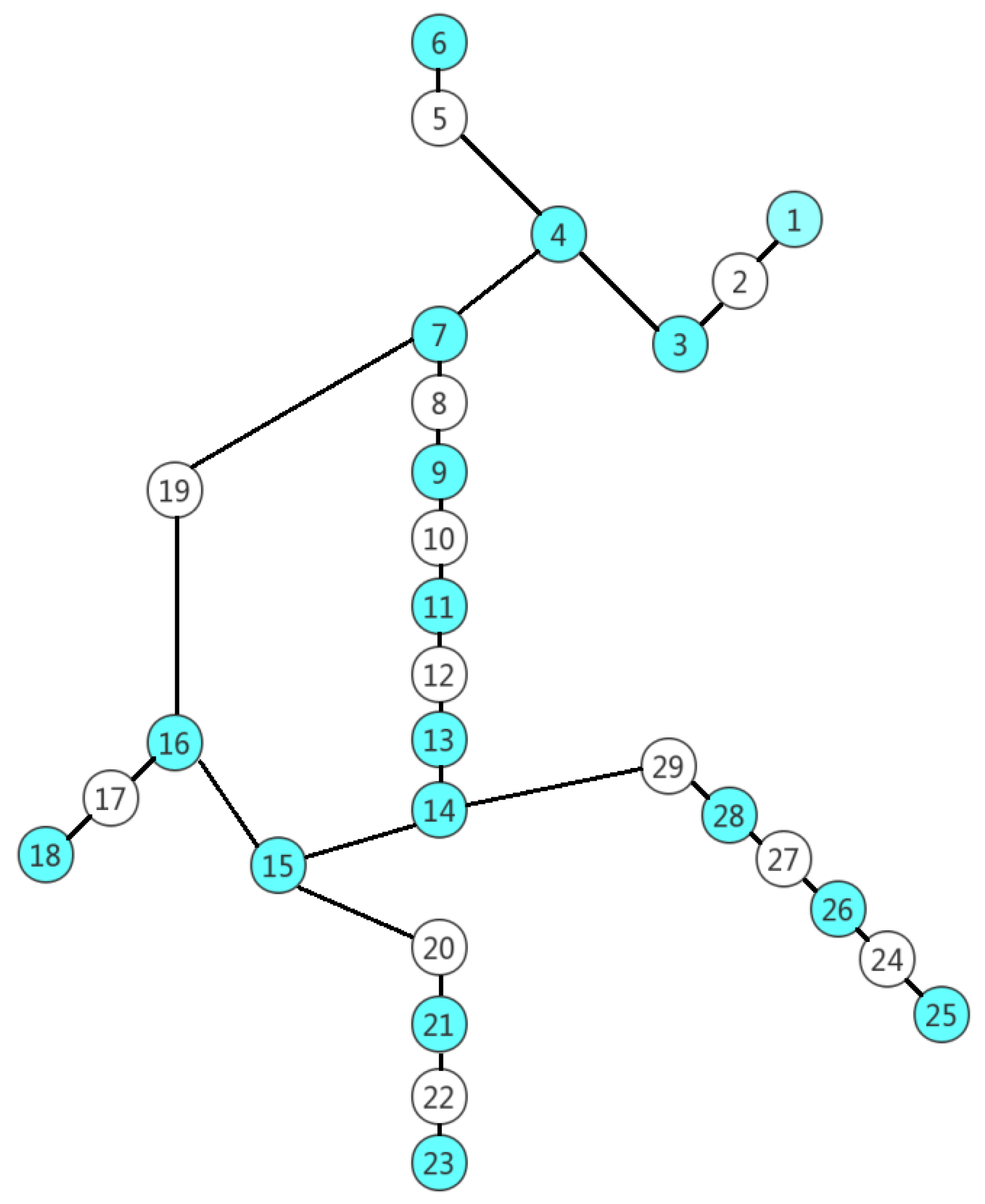
In topology, the number of branches connected to the node is called the degree (d) of the node. Obviously, the degree of an L-type node (node 4 in Figure 1) is 2 and the degree of a T-type node (node 4 in Figure 2) is 3. For general GIS, the node with the largest degree is the cross node, of which the degree is 4, and the node with the smallest degree is the terminal node, of which the degree is 1. The cross node can be considered as the combination of two L-type nodes. To effectively detect the EM wave of PD, the EM wave should not pass through more than one L-type node, one cross node, or one T-type node. These three nodes are collectively called the nonterminal node, of which the degree is greater than or equal to 2.

The number of branches included in the shortest path of node i to node j is defined as the shortest path length P_ij. Under the condition of installing sensors at the terminal node (subject to x_t = 1), a suitable nonterminal node should be selected to install a sensor so that the EM wave passes through, at most, one nonterminal node before reaching the sensors. Therefore, the maximum number of nonconfigurable nodes between any adjacent configurable nodes is 1, and P_ij should be no more than 2 (subject to P_ij = 2). An optimization model can be obtained:

$$\begin{array}{l}\min {\displaystyle \sum _{k=1}^N{x}_k}\\ \mathrm{s}.\mathrm{t}. P_{ij}\le 2\\ \hspace{1em}\hspace{1em}{x}_t=1\end{array}$$

(1)

where t is terminal node, i and j are adjacent nodes, and x_k is the node in which the sensor should be installed. Because the configurable node is unknown, the inequality constraint of the shortest path which contains variable x_k cannot be obtained directly.

The condition above can be described as follows: at least one sensor should be installed on those nodes of which the shortest path length to node k is 1 or 2.

For a node k, an adjacent node matrix V^k is proposed. V^k is M × N matrix, where N is the number of nodes and M is the number of the nodes, of which the shortest path length to the node k is 2. The nodes of which the shortest path length is 1 don’t need to be considered because the shortest path from these M nodes to the node k includes them. For a row vector v of V^k and j (1 ≤ j ≤ N), when P_kj = 1 or P_kj = 2, v_j = 1 and other elements are 0. Therefore, it forms the constraint that at least one sensor should be installed on the path from the node k to the node of which the shortest path length is 2. V^1~N is arranged in columns to form a new matrix V_M×N, and it can be found as follows:

$$V_{M\times N}{X}_{N\times 1}\ge I_{M\times 1}$$

(2)

where X^T = [x₁, x₂, …, x_N] is the vector to be solved and I_M×1 is [1, 1, …, 1]^T.

Reference [27] has proposed the critical point of EM wave propagation. When the values of the critical points are only 0 or 1, the maximum observability can be achieved. The critical points divide the whole system into several sections. R detectable sections are produced; then, the propagation path of the EM wave can be obtained by the topological structure and section length of the GIS. Therefore, a constraint can be found to be

$${\mathit{G}}_{2R\times N}{\mathit{X}}_{N\times 1}\ge {\mathit{I}}_{2R\times 1}$$

(3)

where G is the propagation path matrix of EM wave of each section and the constraint shows that at least one path of the EM wave to the node where the sensor is installed passes through both ends of the section and I_2R×1 = [1, 1, …, 1]^T.

By Equations (2) and (3), the 0-1 optimization model can be obtained:

$$\begin{array}{l}\min W_{1\times N}^T{X}_{N\times 1}\\ \mathrm{s}.\mathrm{t}. V_{M\times N}{X}_{N\times 1}\ge I_{M\times 1}\\ \hspace{1em}\hspace{1em}{\mathit{G}}_{2R\times N}{\mathit{X}}_{N\times 1}\ge {\mathit{I}}_{2R\times 1}\\ \hspace{1em}\hspace{1em}{B}_{2N\times N}{X}_{N\times 1}=b_{2N\times 1}\end{array}$$

(4)

where W^T = [w₁, w₂, …, w_N] is a weight vector and represents the tendency of each node to install a sensor. The elements values of W^T are between 0 and 1. The equation constrains whether if a sensor should be installed at a certain node. If it should be installed at the node k, B(k, k) = 1 and b(k) = 1, otherwise B(k + N, k) = 1. The remaining elements in B and b are 0. The model conforms to the standard form of the 0-1 programming model and it can be solved by using brintprog tool in MATLAB.

2.3. Initial PD Location Method

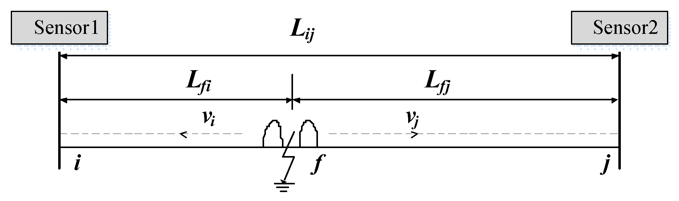
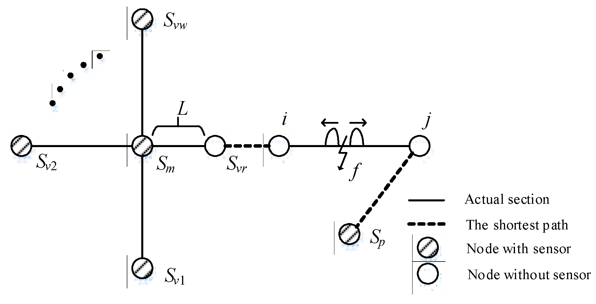
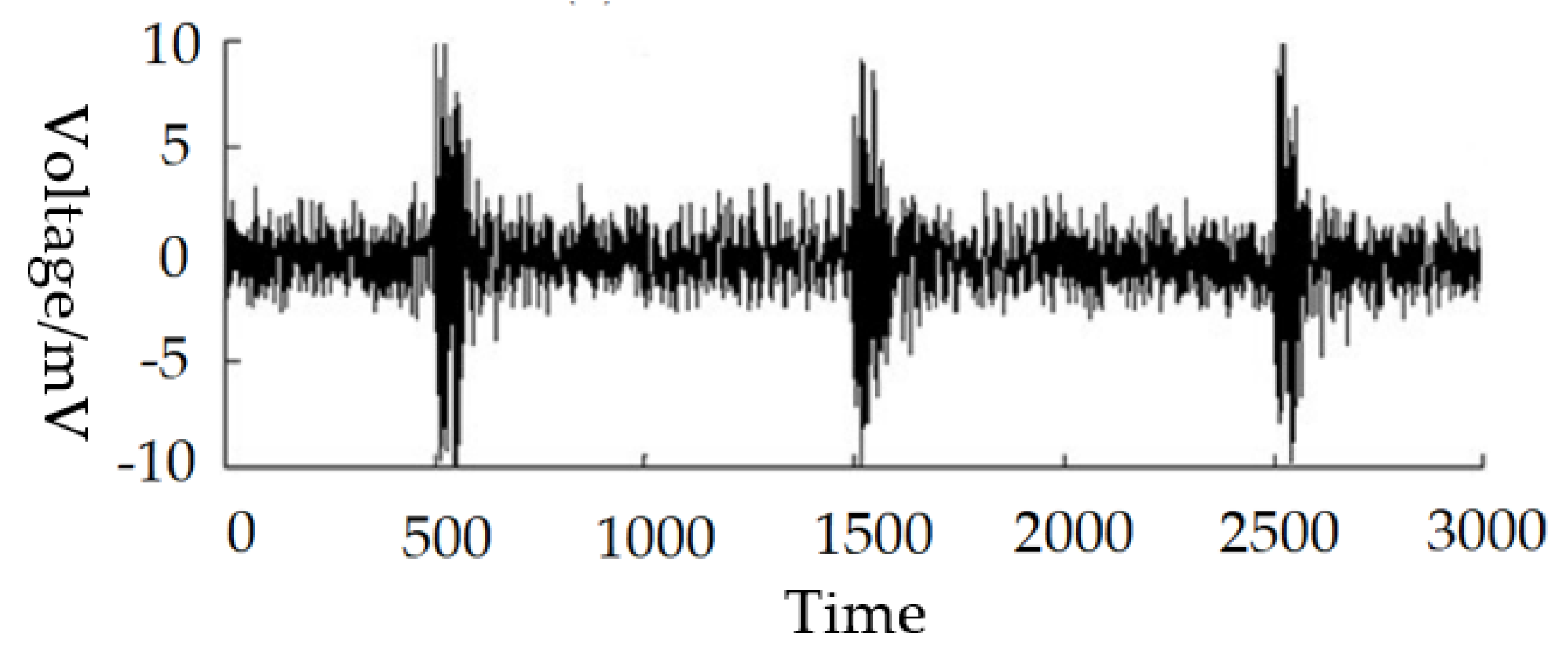
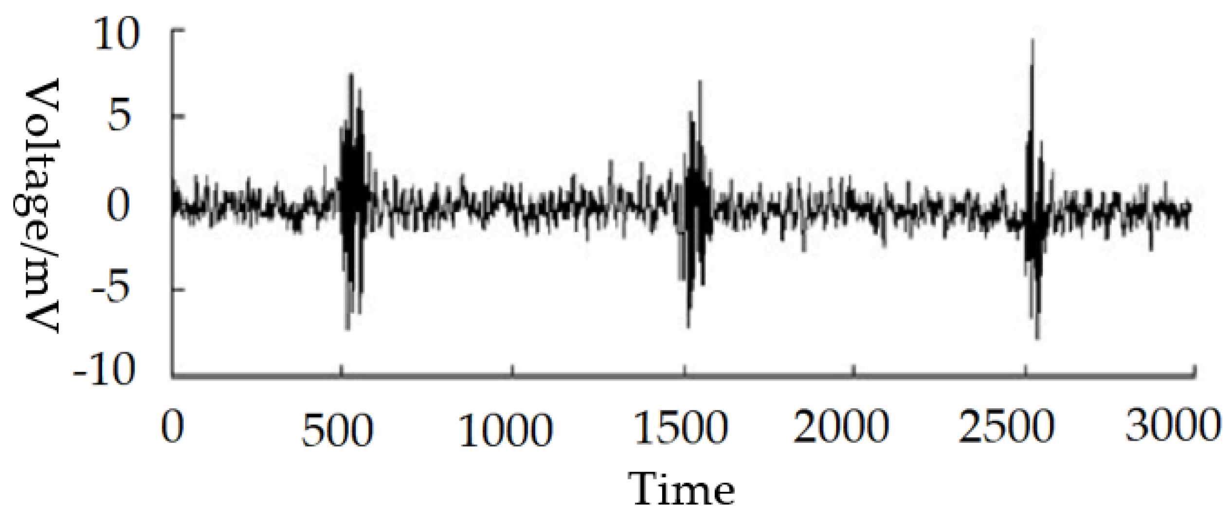
The time difference of arriving location method for GIS is based on the arriving time of the EM signals detected by UHF sensors installed at both ends of the PD section. Considering the outer radius of the cavity of GIS is much smaller than its total length, it can be assumed that the EM wave will travel along the path as the pattern in Figure 3 after PD occurs.

For Figure 3, v_i = v_j = c = 0.3 m/ns is the propagation velocity of the EM wave, and the fault distance from the PD position to sensor 1 is given by

$$L_{fi}=\frac{1}{2}[L_{ij}+(t_i-t_j)c]$$

(5)

$$L_{fj}=L_{ij}-L_{fi}$$

(6)

where L_fi and L_fj are the distance from the PD position to I and to j, t_i and t_j are the time when sensor I and sensor j detect the signals. Equation (5) is a conventional PD location method, and the PD signals can propagate to other sensors through I and j. In view of the integrity of GIS, the propagation velocity of EM wave can be considered as remaining constant. This method lays a foundation for accurate PD locating using multiple sensors in GIS. 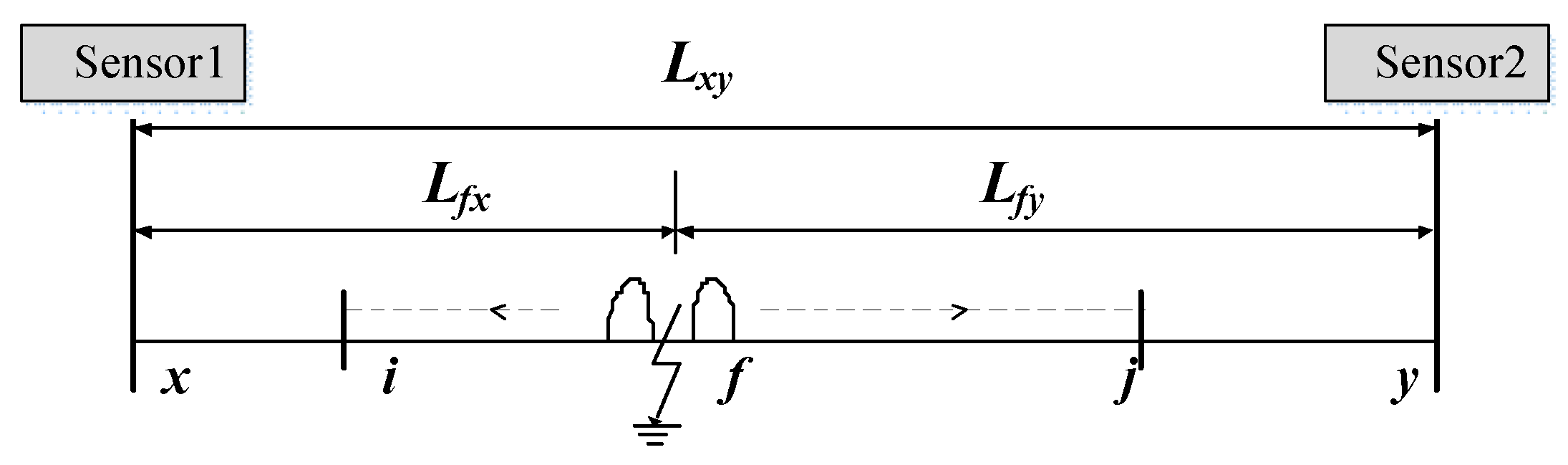Figure 3 can be expanded to Figure 4 below, and the EM waves travel through I and j to adjacent sensor x and y. Replacing I and j with x and y in Equations (5) and (6), the distance of extended TDOA can be expressed as

$$L_{fx}=\frac{1}{2}[L_{xy}+(t_x-t_y)c]$$

(7)

$$L_{fy}=L_{xy}-L_{fx}$$

(8)

Similarly, taking x and j or i and y as the ends of section, the corresponding PD position can be obtained. The extended TDOA method is the basic principle for PD locating of complex GIS. The accurate timing of optical fiber connection and the synchronization of different sampling units to picoseconds are the basis of PD locating among multiple sensors.

By the optimization Equation (4), it is assumed that P UHF sensors are installed at the nodes S = [S₁S₂S₃…S_P] of a GIS. After PD occurs, the arriving time of the EM waves detected by the UHF sensors is T_M = [T₁T₂T₃…T_P]^T and the minimum time in T_M is T_min. For a node S_m in S, all adjacent nodes are S_V = [S_vS_v2S_v3…S_vw], where w is the number of adjacent nodes. In Figure 5, S_vr can be any node in S_V.

The UHF sensors at S_m and S_p form a time difference location combination when PD occurs between i and j, and the shortest path between the two nodes must pass through an adjacent section L of S_m. The other end of L is the node S_vr. For S_m and its adjacent node matrix S_V, w TDOA location combinations can be obtained. For the UHF sensor arrangement matrix S, P – 1 combinations can be obtained. Therefore, the approximate solution can be obtained by comparing the similarity between the transmission time of the EM wave from the PD position to the sensors and the arriving time of the EM wave acquired by sensors synchronously.

The Euclidean distance is used to compare the similarity between two vectors. The Euclidean distance can magnify the error caused by sensor communication and data processing. It is suitable for comparing the unknown quantity with the known quantity with possible error and detecting redundancy. The value of the Euclidean distance is inversely proportional to the similarity between the two sets of data. The more similar the two sets of data are, the smaller the value is. Therefore, the initial locating results of PD can be obtained.

By the shortest path algorithm, the time matrix D_f of the EM waves propagating from the w × (P – 1) positions to UHF sensors can be found as

$$D_f=\begin{array}{cc}& \begin{array}{cccc}\hspace{1em}\hspace{1em}1& \hspace{1em}\hspace{1em} 2& \hspace{1em}\hspace{1em}\cdots & \hspace{1em} w\end{array}\hfill \\ \begin{array}{c}1\\ 2\\ ⋮\\ P-1\end{array}& \left(\begin{array}{cccc}{D}_{11}& D_{12}& \cdots & D_{1w}\\ D_{21}& D_{22}& \cdots & D_{2w}\\ ⋮& ⋮& \ddots & ⋮\\ D_{(P-1)1}& D_{(P-1)2}& \cdots & D_{(P-1)w}\end{array}\right)\end{array}$$

(9)

where the matrix element D_ij = [D_1′ D_2′^… D_P^’]. Furthermore, the distance measure matrix E can be built as

$$\mathit{E}=\begin{array}{cc}& \begin{array}{cccc}\hspace{1em}\hspace{1em}1& \hspace{1em}\hspace{1em}2& \hspace{1em} \cdots & \hspace{1em}w\end{array}\hfill \\ \begin{array}{c}1\\ 2\\ ⋮\\ P-1\end{array}& \left(\begin{array}{cccc}{E}_{11}& E_{12}& \cdots & E_{1w}\\ E_{21}& E_{22}& \cdots & E_{2w}\\ ⋮& ⋮& \ddots & ⋮\\ E_{(P-1)1}& E_{(P-1)2}& \cdots & E_{(P-1)w}\end{array}\right)\end{array}=\begin{array}{cc}& \begin{array}{cccc}\hspace{1em}\hspace{1em}\hspace{1em}\hspace{1em}1& \hspace{1em}\hspace{1em}\hspace{1em}\hspace{1em}\hspace{1em}\hspace{1em}2& \hspace{1em}\hspace{1em}\hspace{1em}\cdots & \hspace{1em}\hspace{1em}\hspace{1em}w\end{array}\hfill \\ \begin{array}{c}1\\ 2\\ ⋮\\ P-1\end{array}& \left(\begin{array}{cccc}\Vert D_{11}-T_{\mathrm{M}}\Vert & \Vert D_{12}-T_M\Vert & \cdots & \Vert D_{1w}-T_M\Vert \\ \Vert D_{21}-T_M\Vert & \Vert D_{22}-T_M\Vert & \cdots & \Vert D_{2w}-T_M\Vert \\ ⋮& ⋮& \ddots & ⋮\\ \Vert D_{(P-1)1}-T_M\Vert & \Vert D_{(P-1)2}-T_M\Vert & \cdots & \Vert D_{(P-1)w}-T_M\Vert \end{array}\right)\end{array}$$

(10)

The initial PD location result is given by the minimum value in the measure matrix E, and the corresponding PD position can be expressed as f′.

2.4. Accurate PD Location Method for GIS

The accuracy of PD locating can be improved by using the information of all UHF sensors installed in GIS. From the initial PD position and the inherent topological structure of GIS, the time of PD occurrence can be calculated. Then, the time of the EM wave propagating to UHF sensors is calculated by the time of PD occurrence and the EM wave velocity to obtain multiple sets of PD location results. With these results, accurate PD locating can be achieved.

The occurring time t₀ of PD can be found to be

$$Tmin-t_0=\frac{L_{{bf}^{\prime }}}{c}$$

(11)

where L_bf’ is the distance from the PD position to the UHF sensor corresponding to T_min. By t₀, the distance matrix of the PD signals propagating to each sensor can be calculated to be

$$\begin{array}{ll}\mathit{L}& =[\begin{array}{cccc}{L}_{1f}& L_{2f}& \cdots & L_{Pf}\end{array}{]}^{\mathrm{T}}\\ & =c(T_M-t_0\mathit{\eta })\end{array}$$

(12)

where η = [1 1 ⋯ 1]^T_P×1. According to the topological structure of GIS, the PD positions can be found:

$$\mathit{S}={\left[\begin{array}{cccc}{S}_1& S_2& \cdots & S_P\end{array}\right]}^{\mathrm{T}}$$

(13)

In combination with all the information of UHF sensors, the accurate PD position can be found as follows:

$$S_{act}=\frac{1}{P}{\displaystyle \sum _{i=1}^P{S}_i}$$

(14)

The flow chart of the PD location method for GIS and the steps are as follows (shown in Figure 6):

1)

Acquire the EM wave arriving time matrix T_M = [T₁T₂T₃…T_P]^T and the corresponding node matrix S = [S₁S₂S₃…S_P] from UHF sensors after PD occurs.

2)

Based on S_m corresponding to T_min, w × (P – 1) PD location combinations are composed of w adjacent nodes and P – 1 UHF sensors.

3)

The initial PD position can be calculated by the measure matrix E, and the occurring time t₀ of PD can be found.

4)

Combining t₀ with the topology structure of GIS, the PD position can be revised by multiple sensors of the GIS to obtain the accurate PD location results.

2.5. Noise Reduction Method

An improved dual-tree complex wavelet transform (DTCWT) method is proposed to reduce noise. The DTCWT method is used to decompose the noisy signal into a series of detail components which can reflect PD [28]. However, only part of DTCWT components details are closely related to PD, while the others are reflected in noise signals. Therefore, the improved DTCWT method is proposed to select sensitive components according to time-domain kurtosis and envelope spectral kurtosis. According to the principle of maximum kurtosis deconvolution, the sensitive components are deconvoluted to reduce noise by MKD deconvolution. Finally, the denoised components are reconstructed by inverse DTCWT transform to obtain the denoised signal.

The steps of the improved DTCWT method are as follows:

1)

Determine the number of decomposition layers of DTCWT. Different layers will affect the accuracy and speed of noise reduction calculation.

2)

Decompose the noisy signal by DTCWT. The signal is transformed by n-layer dual-tree complex wavelet transform. The inverse transform of the wavelet coefficients $wi=w_i^{re}+i{w}_i^{im}$ of layer i is implemented to obtain the wavelet components of layer i. A matrix can be formed by signal components at different scales of signal transformation:

$$Dn=\left(\begin{array}{c}D1\\ D2\\ ⋮\\ Dn\end{array}\right)\left(\begin{array}{cccc}{d}_1(1)& d_1(2)& \cdots & d_1(k)\\ d_2(1)& d_2(2)& \cdots & d_2(k)\\ ⋮& ⋮& & ⋮\\ d_n(1)& d_n(2)& \cdots & d_n(k)\end{array}\right)$$

(15)

3)

Screen Signal Components. The time kurtosis of signal D_i can be found:

$$Kur(d)=\frac{\frac{1}{n}{{\displaystyle \sum (d_i-\overline{d})}}^4}{Std{(x)}^4}$$

(16)

The envelope spectral kurtosis can be found:

$$env(t)=\sqrt{x{(t)}^2+{\{HT[x(t)]\}}^2}$$

(17)

where HT is Hilbert transform. The higher time kurtosis and envelope spectral kurtosis indicate that there are more partial discharge impulse components in D_i. The product of time domain kurtosis and envelope spectral kurtosis (index TE) of each component is calculated, and the component with large product is selected for reconstruction.

4)

The selected DTCWT detail signal component is processed by MKD denoising, and then the inverse DTCWT transform is used to reconstruct the signal. After the inverse transform, the denoised signal of the component can be obtained.

3. Experimental Results and Analysis

3.1. Experimental Platform

The experiment is based on the partial discharge online monitoring system of China Electric Power Research Institute. The precise timing system with optical fiber connection can ensure that the clocks of each sensor can be synchronized to the same nanosecond to realize a precise location system composed of multiple channels. The test system consists of 500 kV GIS model, power supply, PD detector, phase acquisition device, built-in UHF sensor, UHF amplifier, broadband oscilloscope, discharge model, etc (shown in Figure 7 and Figure 8).

The whole experimental GIS platform is divided into independent test chambers by pelvic insulators. Operating hand holes are opened on the side of each chamber to facilitate the placement of defect models, such as a pin-to-plate discharge model.

3.2. Noise Reduction

The noise reduction method is validated by a measured partial discharge signal with noise shown in Figure 9.

The improved DTCWT method is used to denoise the measured partial discharge signal. The sampling number of UHF signal is 3000. The decomposition level of DTCWT is 5. The signal components of DTCWT, of which the TE values are in the top three, are reconstructed. The noise reduction result is shown in Figure 10.

Variation trend parameter (VTP) and signal-to-noise ratio (SNR) are used to evaluate the denoising effect of UHF PD signals:

$$SNR=20\lg \frac{\underset{i=1}{\overset{n}{\max }}s(i)}{\underset{i=1}{\overset{n}{\max }}n(i)}$$

(18)

$$VTP=\frac{{\displaystyle \sum _{i=2}^n[f(i)-f(i-1)]}}{2{\displaystyle \sum _{i=2}^n[s(i)-s(i-1)]}}+\frac{{\displaystyle \sum _{i=2}^n[f(i-1)-f(i)]}}{2{\displaystyle \sum _{i=2}^n[s(i-1)-s(i)]}}$$

(19)

The closer the VTP value is to 1, the better the waveform fitting effect is. Comparing the DTCWT method with improved DTCWT method, the result is shown in

Table 1. The comparison of output variation trend parameter (VTP) and signal-to-noise ratio (SNR).

	DTCWT	Improved DTCWT
SNR	7.59	20.07
VTP	1.495	1.030

. The improved DTCWT method has higher SNR and the waveform is not obviously distorted, which maintains the characteristics of the original UHF PD signal.

3.3. Optimal Placement

The 500 kV GIS experimental platform was used to verify the effectiveness of the proposed method. The nodes of GIS are numbered and the node number is also the sensor number. The lengths of the sections between the nodes are shown in

Table 2. GIS topological parameters.

Section	Length (mm)	Section	Length (mm)
1–2	3826	16–17	1060
2–3	1705	17–18	3413
3–4	1153	16–19	1715
4–5	2494	19–7	3380
5–6	1155	15–20	1035
4–7	1550	20–21	1380
7–8	1133	21–22	2860
8–9	3485	22–23	1380
9–10	2550	23–24	1060
10–11	8210	24–25	1250
11–12	2550	24–26	3460
12–13	3485	26–27	990
13–14	1740	27–28	990
14–15	3380	28–29	3790
15–16	1715	29–14	1740

.

The undirected graph of the structure of this GIS shown in Figure 11 can be drawn from Table 2. The nodes where UHF sensors should be installed can be obtained by model (4), including nodes 1, 3, 4, 6, 7, 9, 11, 13, 14, 15, 16, 18, 21, 23, 25, 26, and 28. In Figure 11, the system has two tangent ring structures; therefore, non-detection zones may exist. The minimum and maximum values of the EM wave critical points for all sections are 0 and 1 through calculations [27]. Therefore, these sections are totally detectable. In addition, the constraints of model (4) ensure that the sensors can detect the EM waves effectively.

3.4. PD Location Results

Assume a PD occurred at 20 ns in section 8‒9, and the distance from the PD position to node 8 is 1000 mm. Each sensor can monitor the signal of each node and 400 MHz high-pass filtering was performed on the EM signal detected by the sensors. The amplitude and waveform of the signal barely change through the filter, so it is easy to obtain the arriving time of the EM wave, as shown in

Table 3. Arriving time of the initial signal.

Sensor Number	Time (ns)	Sensor Number	Time (ns)
1	34.7	15	29.3
3	15.7	16	24.3
4	12.6	18	39.4
6	24.3	21	37.3
7	7.3	23	52.5
9	7.9	25	59.4
11	43.8	26	66.6
13	47.2	28	59.1
14	40.5	--	--

. From Table 2, T_min = t₇. Calculating the TDOA of sensor 7 with the other 16 sensors in sequence, the results are shown in

Table 4. Initial results of PD locating.

Sensor Combination	Euclidean Distance	PD Section	PD Position (mm)
(1,7)	8.9	3‒4	7.0 × 10−2
(3,7)	6.8	4‒7	1.2 × 10−1
(4,7)	7.0	4‒7	2.4 × 10−1
(6,7)	8.8	5‒6	1.2
(9,7)	1.9	8‒9	915.0
(11,7)	0.8	8‒9	954.3
(13,7)	2.3	8‒9	1113.4
(14,7)	1.9	8‒9	903.5
(15,7)	1.7	8‒9	954.3
(16,7)	1.8	8‒9	915.0
(18,7)	3.9	4‒5	1.3 × 10-3
(21,7)	1.7	8‒9	923.5
(23,7)	2.1	8‒9	903.5
(25,7)	1.2	8‒9	1078.2
(26,7)	1.9	8‒9	915.0
(28,7)	1.8	8‒9	1093.4

. In Table 4, the minimum value in the Euclidean distance measure matrix corresponds to the result calculated by sensor 7 and 11. Therefore, the PD occurred in section 8‒9, 954.3 mm away from node 8. The actual discharge distance is 1000 mm, the absolute error is 45.7 mm, and the relative error is 4.6%. The occurring time t₀ of PD was found to be 20.1 ns by Formula (12). Based on Formulas (13) and (14), the revised PD position can be obtained shown in

Table 5. Revised results of PD locating.

Sensor Number	PD Position (mm)	Absolute Error (mm)
1	1098.4	98.4
3	1123.9	123.9
4	1087.0	87.0
6	923.5	76.5
7	883.5	116.5
9	1095.8	95.8
11	913.9	86.1
13	913.4	86.5
14	954.3	45.7
15	902.7	97.3
16	906.6	93.4
18	1087.9	87.9
21	1077.2	77.2
23	923.5	76.5
25	893.7	106.3
26	914.2	85.8
28	1092.6	92.6

. By Formula (15), the PD occurred in section 8‒9, 993.5 mm away from node 8. The actual discharge distance is 1000 mm, the absolute error is 6.5 mm, and the relative error is 0.7%.

3.5. Fault Tolerance Analysis

The proposed method has been verified in the example above on PD of 500 kV GIS, but the PD locating is under the premise that there is no error in the detection of the UHF sensors. In practical operation, error data of sensors would be caused by the influence of environmental noise and communication delay.

In order to verify the fault tolerance of the algorithm, the arriving time of the EM wave of the sensor at node 11 was artificially set as 53.8 ns. The minimum arriving time T_min remains t₇, and the TDOA calculations of sensor 7 with the other sensors in sequence were carried out. The result shows that the PD distance calculated by the combination of senor 7 and 11 is infinity. Therefore, the information obtained by sensor 11 was judged to be erroneous data. After the erroneous data was eliminated, it can be obtained that the PD occurred on section 8‒9, 988.7 mm away from node 8. The absolute error is 11.3 mm and the relative error is 1.1%.

In the same case, the existing methods for PD locating cannot eliminate the impact of erroneous data. The proposed method realizes the identification of the erroneous data through the information of multiple sensors in GIS and ensures the fault tolerance of the algorithm.

3.6. Comparison of Methods

The received signal strength indicator (RSSI) location method is based on the strength of EM wave. PD locating can be achieved by the reconstruction algorithm of RSSI based on pattern matching [29,30]. Twelve experiments were carried out to compare the proposed method and the RSSI method. Location results are shown in

Table 6. Method comparison.

	Proposed Method	RSSI
average absolute error (mm)	22.8	107.7
absolute error < 50 mm (%)	100	50
absolute error < 100 mm (%)	100	66.7
absolute error < 200 mm (%)	100	83.3
Maximum absolute error (mm)	42.3	238.5

.

For Table 6, The average absolute error of the proposed method is 22.8 mm, which is obviously superior to the RSSI method, and its 100% absolute errors are less than 50 mm. The proposed method keeps the ns-level time synchronization between the sensors and the acquisition system. Therefore, the precision and accuracy can be guaranteed.

4. Conclusions

Considering the attenuation of the EM wave when passing through the insulators, L-type and T-type structures in GIS, and the constraints of economy and observability, an optimal placement model of UHF sensors is proposed. The model can meet the requirements and has high reliability, as validated by experimental results.

Based on the optimal placement of the UHF sensors and the arriving time of EM waves, the initial results of PD locating can be calculated by the Euclidean distance and the TDOA method. Then, the accurate results can be calculated by the occurring time of PD and the information of all UHF sensors.

Compared to the existing PD location methods, the proposed method ensures the accuracy and fault tolerance of PD locating. The experimental results show the method has high accuracy and robustness.

References

1. Si, W.R.; Li, J.H.; Li, D.J.; Yang, J.G.; Li, Y.M. Investigation of a Comprehensive Identification Method Used in Acoustic Detection System for GIS. IEEE Trans. Dielectr. Electr. Insul. 2010, 17, 721–732. [Google Scholar] [CrossRef]
2. OKabe, S.; Yamagiwa, T.; Okubo, H. Detection of Harmful Metallic Particles Inside Gas Insulated Switchgear using UHF Sensor. IEEE Trans. Dielectr. Electr. Insul. 2008, 15, 701–709. [Google Scholar] [CrossRef]
3. OKabe, S.; Ueta, G.; Hama, H.; Ito, T.; Hikita, M.; Okubo, H. New aspects of UHF PD diagnostics on gas-insulated systems. IEEE Trans. Dielectr. Electr. Insul. 2014, 21, 2245–2258. [Google Scholar] [CrossRef]
4. Mirzaei, H.R.; Akbari, A.; Gockenbach, E.; Miralikhani, K. Advancing new techniques for UHF PD detection and localization in the power transformers in the factory tests. IEEE Trans. Dielectr. Electr. Insul. 2015, 22, 448–455. [Google Scholar] [CrossRef]
5. Ishak, A.M.; Ishak, M.T.; Jusoh, M.T.; Dardin Syed, S.F.; Judd, M.D. Design and optimazation of UHF partial discharge sensors using FDTD modeling. IEEE Sens. J. 2017, 17, 127–133. [Google Scholar]
6. Wang, Y.; Wang, X.; Li, J. UHF moore fractal antennas for online GIS PD detection. IEEE Antennas Wirel. Propag. Lett. 2017, 16, 852–855. [Google Scholar] [CrossRef]
7. Tenbohlen, S.; Denissov, D.; Hoek, S.M.; Markalous, S.M. Partial discharge measurement in the ultra-high frequency (UHF) range. IEEE Trans. Dielectr. Electr. Insul. 2008, 15, 1544–1552. [Google Scholar] [CrossRef]
8. Xu, Y.; Liu, W.; Gao, W. Investigation of disc-type sensors using the UHF method to detect partial discharge in GIS. IEEE Trans. Dielectr. Electr. Insul. 2015, 22, 3019–3027. [Google Scholar] [CrossRef]
9. Sinaga, H.H.; Phung, B.T.; Blackburn, T.R. Recognition of single and multiple partial discharge sources in transformers based on ultra-high frequency signals. IET Gener. Transm. Distrib. 2014, 8, 160–169. [Google Scholar] [CrossRef]
10. Boya, C.; Rojas, M.V.; Ruiz, M.; Robles, G. Location of partial discharges sources by means of blind source separation of UHF signals. IEEE Trans. Dielectr. Electr. Insul. 2015, 22, 2302–2310. [Google Scholar] [CrossRef]
11. Gao, W.; Ding, D.; Liu, W. Research on the typical partial discharge using the UHF detection method for GIS. IEEE Trans. Power Deliv. 2011, 26, 2621–2629. [Google Scholar] [CrossRef]
12. Zhang, G.B.; Guo, J.B.; Chu, F.H.; Zhang, Y.C. Environmental-adaptive indoor radio path loss model for wireless sensor networks localization. Int. J. Electron. Commun. 2011, 65, 1023–1031. [Google Scholar] [CrossRef]
13. Iorkyase, E.T.; Tachtatzis, C.; Atkinson, R.C.; Glover, I.A. Localization of partial discharge sources using radio fingerprinting technique. In Proceedings of the 2015 Loughborough Antennas & Propagation Conference (LAPC), Loughborough, UK, 2–3 November 2015; pp. 1–5. [Google Scholar]
14. Ito, T.; Kamei, M.; Ueta, G.; Okabe, S. Improving the sensitivity verification method of the UHF PD detection technique for GIS. IEEE Trans. Dielectr. Electr. Insul. 2012, 18, 1847–1853. [Google Scholar] [CrossRef]
15. Reid, A.J.; Judd, M.D.; Fouracre, R.A.; Stewart, B.; Hepburn, D.M. Simultaneous measurement of partial discharges using IEC60270 and radio-frequency techniques. IEEE Trans. Dielectr. Electr. Insul. 2011, 18, 444–455. [Google Scholar] [CrossRef]
16. Zheng, S.; Li, C.; Tang, Z.; Chang, W.; He, M. Location of PDs inside transformer windings using UHF methods. IEEE Trans. Dielectr. Electr. Insul. 2014, 21, 386–393. [Google Scholar] [CrossRef]
17. Hekmati, A.; Hekmati, R. Optimum acoustic sensor placement for partial discharge allocation in transformers. IET Sci. Meas. Technol. 2017, 11, 581–589. [Google Scholar] [CrossRef]
18. Dai, D.; Wang, X.; Long, J.; Tian, M.; Zhu, G.; Zhang, J. Feature extraction of GIS partial discharge signal based on S-transform and singular value decomposition. IET Sci. Meas. Technol. 2017, 11, 186–193. [Google Scholar] [CrossRef]
19. Gao, W.; Ding, D.; Liu, W.; Huang, X. Propagation attenuation properties of partial discharge in typical in-field GIS structures. IEEE Trans. Power Deliv. 2013, 28, 2540–2549. [Google Scholar] [CrossRef]
20. Hikita, M.; Ohtsuka, S.; Wada, J.; Okabe, S.; Hoshino, T.; Maruyama, S. Propagation properties of PD-induced electromagnetic wave in 66 kV GIS model tank with L branch structure. IEEE Trans. Dielectr. Electr. Insul. 2011, 18, 1678–1685. [Google Scholar] [CrossRef]
21. Hikita, M.; Ohtsuka, S.; Ueta, G.; Okabe, S.; Hoshino, T.; Maruyama, S. Influence of insulating spacer type on propagation properties of PD-induced electromagnetic wave in GIS. IEEE Trans. Dielectr. Electr. Insul. 2010, 17, 1642–1648. [Google Scholar] [CrossRef]
22. Li, T.; Wang, X.; Zheng, C.; Liu, D.; Rong, M. Investigation on the placement effect of UHF sensor and propagation characteristics of PD-induced electromagnetic wave in GIS based on FDTD method. IEEE Trans. Dielectr. Electr. Insul. 2014, 21, 1015–1025. [Google Scholar] [CrossRef]
23. Li, X.; Wang, X.; Yang, A.; Xie, D.; Ding, D.; Rong, M. Propogation characteristics of PD-induced UHF signal in 126 kV GIS with three-phase construction based on time-frequency analysis. IET Sci. Meas. Technol. 2016, 10, 805–812. [Google Scholar] [CrossRef]
24. Markalous, S.M.; Tenbohlen, S.; Feser, K. Detection and location of partial discharges in power transformers using acoustic and electromagnetic signals. IEEE Trans. Dielectr. Electr. Insul. 2008, 15, 1576–1583. [Google Scholar] [CrossRef]
25. Tang, J.; Xie, Y. Partial discharge location based on time difference of energy accumulation curve of multiple signals. IET Electr. Power Appl. 2011, 5, 175–180. [Google Scholar] [CrossRef]
26. Zhang, Q.; Li, C.; Zheng, S.; Yin, H.; Kan, Y.; Xiong, J. Remote detecting and locating partial discharge in bushings by using wideband RF antenna array. IEEE Trans. Dielectr. Electr. Insul. 2016, 23, 3575–3583. [Google Scholar] [CrossRef]
27. Liang, R.; Xu, C.; Wang, F.; Cheng, Z.; Shen, X. Optimal deployment of fault location devices based on wide area travelling wave information in complex power grid. Trans. China Electrotech. Soc. 2016, 31, 30–38. [Google Scholar]
28. Le, Q.; Zhen, Z.; Pei, Y. Image identification of insects based on color histogram and dual tree complex wavelet transform (DTCWT). Acta Entomol. Sin. 2010, 53, 91–97. [Google Scholar]
29. Zhang, W.; Bi, K.; Luo, L.; Sheng, G.; Jiang, X. RSSI fingerprinting-based UHF partial discharge localization technology. In Proceedings of the Power & Energy Engineering Conference, Xi’an, China, 25–28 October 2016; pp. 1364–1367. [Google Scholar]
30. Li, Z.; Luo, L.G.; Sheng, G.H.; Liu, Y.; Jiang, X. UHF partial discharge localisation method in substation based on dimension-reduced RSSI fingerprint. IET Gener. Transm. Distrib. 2018, 12, 398–405. [Google Scholar] [CrossRef]
Figure 1. L-type structure of gas-insulated switchgear (GIS).
Energies 12 01173 g001
Figure 2. T-type structure of GIS.
Energies 12 01173 g002
Figure 3. Location method based on time difference of arriving (TDOA).
Energies 12 01173 g003
Figure 4. Extended TDOA location method.
Energies 12 01173 g004
Figure 5. The sensors adjacent to Sm.
Energies 12 01173 g005
Figure 6. Flow chart of the location method.
Energies 12 01173 g006
Figure 7. Partial discharge (PD) online monitoring system diagram.
Energies 12 01173 g007
Figure 8. Laboratory for the PD online monitoring system. (a) Experimental Platform, (b) ultra-high frequency (UHF) sensor in GIS, (c) discharge model in GIS.
Energies 12 01173 g008
Figure 9. Measured partial discharge signal.
Energies 12 01173 g009
Figure 10. Noise reduction result.
Energies 12 01173 g010
Figure 11. Sensor placement results.
Energies 12 01173 g011