Research of the Fundamental Wave of Wound-Rotor Brushless Doubly-Fed Machine

Abstract

The brushless doubly-fed machine (BDFM) is a special type of machine with two sets of stator windings and one set of rotor winding. The magnetic field of the BDFM is considered to be complex with no regularity. To study the principles of magnetic fields for the BDFM, a general expression of the fundamental wave is deduced, which shows that the fundamental wave can be regarded as a standing wave when it is observed from rotor reference; also, some discussions about the characteristics of the fundamental wave are presented in the paper. Next, a model of wound-rotor BDFM prototype is established, and the enveloping line and the relations between rotor position and its electrical angle of the magnetic field are figured out in the paper. Finally, after detecting the induced electromotive force (EMF) of measurement coils embedded in the corresponding prototype machine, the validity of the proposed conclusions is verified.

1. Introduction

The brushless doubly-fed machine (BDFM) is a new type of AC machine which was first proposed in 1905 [1]. The stator winding of a BDFM consists of two sets of three-phase symmetrical windings, one called power winding, which is usually connected to the grid, the other one called control winding; the connection of control winding is not fixable and usually depends on the operation state of the machine. When the machine is going to be operated in the doubly-fed state, the control winding is connected to the converter [2,3]. In addition, as the control winding affords a “slip” part of power in the operation of the machine, a small-capacity converter would be able to control a large-capacity machine which would reduce costs. Due to the above-mentioned advantages, BDFM is increasingly required as ship shaft generators, or in variable speed constant frequency generation systems, such as wind turbine and standalone power systems [4,5].

The rotor in a BDFM is the key aspect in the machine which determines the efficiency of energy conversion. References [6,7,8] proposed some different structures of rotors of BDFMs, and provided some discussions on the performance analysis and reducing the harmonic content, however, the research on the fundamental wave was not mentioned. References [9,10] focused on the analyzing and modeling of the magnetic field in a BDFM with nested-loop rotor; the magnetic field of the BDFM is considered to be complex with no regularity, which results in difficulties in analysis of the principles of the BDFM.

This paper proposes a general expression of the fundamental wave in the gap. The basic form of the fundamental wave should be a standing wave when it is observed from the rotor side. Because of the restriction of rotor design, the amplitudes of two induced fields are different, which leads to the distortion of the final form of the fundamental wave. The relation between angle variation of magnetic force and its corresponding rotor position has also been clarified nonlinear in the paper, and the rapid variation of the angle has been proven related to the stationary point of the standing wave by the simulation. Finally, a 72-stator-slot, 48-rotor-slot prototype machine has been manufactured. By the experiments, the distribution of the fundamental wave in the gap can be observed by using the method of detecting the induced electromotive force (EMF) in measurement coils, and then the proposed expression and theory can be verified.

2. The Design Theory of Wound-Rotor BDFM

According to the basic theory of induction machine windings, when a suit of $p$-pole pair winding is embedded in a machine which has $z$ slots, a special kind of harmonic called tooth harmonic will be produced simultaneously [11,12,13]. The pole pairs of tooth harmonic magnetic potential can be expressed as:

$$\upsilon =nz\pm p \left(n=1,2,3\cdots \right)$$

(1)

where in formula (1), the level of tooth harmonic is closely related to the number of slots. Different from other high-level harmonics, the tooth harmonic cannot be enervated by adjusting the winding coefficient. The distribution coefficient and winding pitch coefficient of an $n$-level tooth harmonic can be calculated as:

$$k_{yt}=sin\left(\frac{\upsilon }{p}·\frac{y}{\tau }·\frac{\pi }{2}\right)=sin\left[\left(\frac{nz}{p}+1\right)·\frac{y}{\tau }·\frac{\pi }{2}\right]=sin\left(ny\pi \pm \frac{y\pi }{2\tau }\right)=\pm k_{yp}$$

(2)

$$k_{qt}=\frac{sin\left(b·\frac{\upsilon \alpha }{2}\right)}{b·sin\left(\frac{\upsilon \alpha }{2}\right)}=\frac{sin\left(\frac{bnz\alpha \pm bp\alpha }{2}\right)}{b·sin\left(\frac{nz\alpha \pm p\alpha }{2}\right)}=\frac{sin\left(sbn\pi \pm \frac{bp\alpha }{2}\right)}{b·sin\left(sn\pi \pm \frac{p\alpha }{2}\right)}=\pm k_{qp}$$

(3)

Statement (2) and (3) [12,13] have demonstrated the special property of tooth harmonics. Conclusions can be derived from the statements above, that the winding coefficient of the tooth harmonic wave and the fundamental wave shares a same value, that is, it is unrealistic to weaken the tooth harmonic wave by enervating its coefficient. On the other hand, considering the specialty of two components of the fundamental wave of BDFM, the design theory of two magnetic potentials can reference the theory of tooth harmonics.

From the expression of the level of tooth harmonics, it can be concluded that for a $z$-slot machine, when $z$ equals $p_p+p_c$, the $p_p$-pole-pair magnetic potential and $p_c$-pole-pair magnetic potential can be treated as a one-level tooth harmonic wave, while the other one is set as the fundamental wave symmetrically, which is the basic theory of designing the stator and rotor windings of BDFM. However, considering the negative influence of leakage magnetic flux, the rotor slot number of BDFM $z$ is often several times the sum of $p_p$ and $p_c$. Figure 1 lays out a rotor winding scheme of a BDFM with a set of 2-pole-pair stator power winding and a set of 4-pole-pair stator control winding. In this BDFM, $p_p=2$ and $p_c=4$. The number in this figure indicates the serial number of the stator slot at which the upper side of the corresponding coil is assembled. In the scheme, the rotor slot number $z$ is 8 times of $p_p+p_c$.

3. Fundamental Wave Magnetic Field Analysis

As it is known, the magnetic field of a BDFM is combined by two sets of stator magnetic fields, thus a rotor magnetic field, which, excited by the corresponsive rotor structure, should contribute a magnetic field in order to match the fields created by the stator. If an electrical machine can be operated stably and smoothly, two magnetic fields, which are separately produced by stator and rotor, should be operated in same frequency and same rotating speed. In order to achieve this goal, analyzing two magnetic fields to express its immanent operating characteristics clearly is necessary.

The following assumptions are made to research the magnetic fields in the air gap:

• The magnetic conductivity of the magnetic materials in the machine is constant, which eliminates the interference of magnetization curve saturation in the material, indicating that the corresponding relation of flux density B and the magnetic density H is linear.
• The impacts of leakage magnetic flux and the impedance of all the windings are omitted.
• The harmonic components are neglected; the main fundamental wave in the air gap is chosen to be observed.

As a BDFM operates in synchronous mode, the power winding and the control winding are connected to different excitations separately. From the stator side, the frequency and the pole pairs of two magnetic fields excited by two sets of windings are totally different. The expression of the combined magnetic field is [14]:

$$F=F_{p}cos\left({\omega }_{p}t-p_p\theta \right)+F_{c}cos\left({\omega }_{c}t+p_c\theta \right)$$

(4)

The variation $F_p$ and $F_c$ can be described as: [15]

$$F_p=\frac{\sqrt{2}{m}_s{N}_{sp}{K}_{wsp}{I}_{mp}}{\pi p_p}$$

(5)

$$F_c=\frac{\sqrt{2}{m}_s{N}_{sc}{K}_{wsc}{I}_{mc}}{\pi p_c}$$

(6)

However, all the statements are based on the three-phase stationary coordinate system; considering the complex description of the combined magnetic field and the relations between magnetic fields angle frequency and the rotor speed, it is necessary to convert the coordinate system to the rotor, since it is a better choice to set the coordinate to rotate with rotor synchronously. As the two sets of stator winding share one set of rotor winding, the ratio of $F_p$ and $F_c$ can be expressed as [15]:

$$\frac{F_p}{F_c}=\frac{p_c{K}_{wrp}}{p_p{K}_{wrc}}$$

(7)

Two $K_{wr}$ coefficients represent the corresponding winding coefficient of rotor windings, therefore two expressions of fundamental wave magnetic fields of stator power windings and control windings after current conversion and coordinate transformation are:

$$F=F_{p}cos\left[{\omega }_{r}t-\left(p_p{\theta }_r+{\phi }_0\right)\right]+F_{c}cos\left[{\omega }_{r}t+\left(p_c{\theta }_r+{\phi }_0\right)\right]$$

(8)

It should be noticed that in the formal statement of two magnetic potentials, initial angle is taken into consideration. Considering that it is impossible to guarantee two initial angles of potential to stay the same, consuming an initial angle in the statement is necessary. In the statement, the initial angles are set as ${\phi }_0$ and $-{\phi }_0$ separately.

In the assumption of two potentials, the amplitude of two components is unequal. Here an assistant coefficient $k_{amp}$ is defined, representing the ratios of amplitudes of two stator magnetic fields. Considering that:

$$F_p=k_{amp}·F_c$$

(9)

the combined magnetic potential in the air gap can be derived as:

$$F=F_{p}cos\left[{\omega }_{r}t-\left(p_p{\theta }_r+{\phi }_0\right)\right]+k_{amp}·F_{p}cos\left[{\omega }_{r}t+\left(p_c{\theta }_r+{\phi }_0\right)\right]$$

(10)

By using trigonometric transformation,

$$\begin{gathered} F=F_p·\{cos{\omega }_{r}t·\left[cos\left(p_p{\theta }_r+{\phi }_0\right)+k_{amp}·cos\left(p_r{\theta }_r+{\phi }_0\right)\right] \\ +sin{\omega }_{r}t·\left[sin\left(p_p{\theta }_r+{\phi }_0\right)-k_{amp}·sin\left(p_r{\theta }_r+{\phi }_0\right)\right]\} \end{gathered}$$

(11)

The final form of combined magnetic field is:

$$\begin{gathered} F=\sqrt{1+k_{amp}^2+2k_{amp}·cos\left[\left(p_p+p_c\right){\theta }_r+2{\phi }_0\right]}·F_p \\ cos\left[{\omega }_{r}t-{cos}^{-1}\frac{cos\left(p_p{\theta }_r+{\phi }_0\right)+k_{amp}·cos\left(p_c{\theta }_r+{\phi }_0\right)}{\sqrt{1+k_{amp}^2+2k_{amp}·cos\left[\left(p_p+p_c\right){\theta }_r+2{\phi }_0\right]}}\right] \end{gathered}$$

(12)

Expression (12) is also the general expression of combined fundamental wave magnetic potential in the BDFM. In this expression, the parameter ${\phi }_0$ appears in two situations. The one in the part of amplitude may cause the offset of the whole figure, while the other ${\phi }_0$ takes the influence on the detailed shape of the curve at a different moment. However, it should be pointed out that different ${\phi }_0$ just leads to the different offset when it is compared to the situation of ${\phi }_0=0$. The following discussion will ignore the influence of ${\phi }_0$ (i.e., the situation of ${\phi }_0=0)$.

From this expression, some basic conclusions can be drawn as follows:

As the maximum value of a pure cosine expression is no bigger than 1, the part $\sqrt{1+k_{amp}^2+2k_{amp}·cos\left[\left(p_p+p_c\right){\theta }_r+2{\phi }_0\right]}·F_p$ in the expression indicates the envelope line of whole lines of different moment. This line is a position-angle-related function as the parameter $k_{amp}$ is determined during the machine design. The maximum value of this function is $\left(1+k_{amp}\right)·F_p=F_p+F_c$, while the minimum is $\left|1-k_{amp}\right|·F_p=\left|F_p-F_c\right|$. 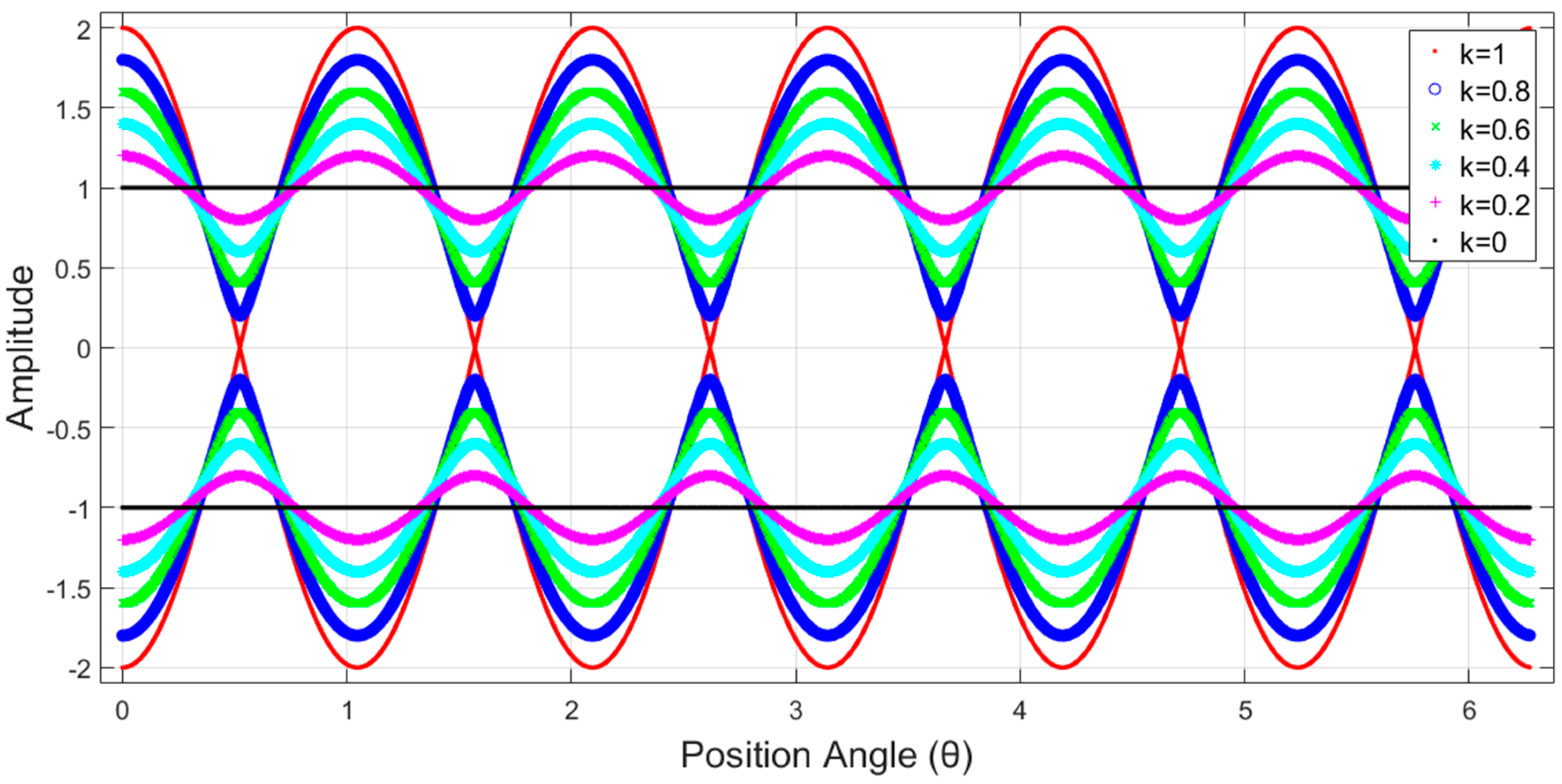Figure 2 shows the detailed shape of the envelope line when parameter $k_{amp}$ differs.

In Figure 2, $p_p$ is set by 4, while $p_c$ is set by 2. It is obvious that due to the characteristics of $cos 6\theta$, this expression has six maximums and six minimums during the whole $2\pi$ period in the machine. The number of extremum points is decided by the sum of $p_p+p_c$. As $k_{amp}$ varies from 1 to 0, the corrugating amplitude gets smaller and smaller, while the minimum point can be reached as zero when $k_{amp}$ takes the value of 1 (i.e., $F_p=F_c)$. If the envelope line of a BDFM can be portrayed by using a quantity of magnetic potential distribution lines in different moments, it is easy to derive the amplitudes of two magnetic potentials.

The part ${cos}^{-1}\frac{cos\left(p_p{\theta }_r+{\phi }_0\right)+k_{amp}·cos\left(p_c{\theta }_r+{\phi }_0\right)}{\sqrt{1+k_{amp}^2+2k_{amp}·cos\left[\left(p_p+p_c\right){\theta }_r+2{\phi }_0\right]}}$ is the expression of electrical angle in different positions of the machine. If ${\phi }_0$ is omitted, this will become a nonlinear function of position ${\theta }_r$. The value of this function varies from 0 to $\pi$.

In this situation, what should be pointed out is the special circumstance when $k_{amp}$ takes the value of 1 with no initial angle difference. Considering that the radical part before $F_p$ is a non-negative number, if $k_{amp}=1$, the following statement results:

$$\sqrt{1+1+2·cos\left(p_p+p_c\right){\theta }_r}=\sqrt{4·{cos}^2\left(\frac{p_p+p_c}{2}\right){\theta }_r}=2·\left|cos\left(\frac{p_p+p_c}{2}\right){\theta }_r\right|$$

(13)

Thus, the precise statement of the magnetic field expression is:

$$2·\left|cos\left(\frac{p_1+p_2}{2}\right){\theta }_r\right|·F_p·cos\left({\omega }_{r}t-{cos}^{-1}\frac{cos{p}_p{\theta }_r+cos{p}_c{\theta }_r}{2·\left|cos\left(\frac{p_p+p_c}{2}\right){\theta }_r\right|}\right)$$

(14)

Compared to the traditional expression of a standing wave expression, the influence of $cos\left(\frac{p_p+p_c}{2}\right){\theta }_r$ is combined into the time-varying part of the expression. The envelope line part only represents the norm of every trigonometric function in each position, that is, considering the regular variance of positive or negative sign of $cos\left(\frac{p_p+p_c}{2}\right){\theta }_r$, this function can be written as another piecewise function form:

$$F=\{\begin{array}{l}2·cos\left(\frac{p_p+p_c}{2}\right){\theta }_r·F_1·cos\left({\omega }_{r}t-\frac{p_p-p_c}{2}·{\theta }_r\right),\hspace{1em}\mathrm{when} cos\left(\frac{p_p+p_c}{2}\right){\theta }_r>0\\ 2·cos\left(\frac{p_p+p_c}{2}\right){\theta }_r·F_1·cos\left[{\omega }_{r}t-\left(\pi -\frac{p_p-p_c}{2}·{\theta }_r\right)\right], \mathrm{when} cos\left(\frac{p_p+p_c}{2}\right){\theta }_r<0\\ 0,\hspace{1em}\mathrm{when} cos\left(\frac{p_p+p_c}{2}\right){\theta }_r=0,\hspace{1em}\mathrm{i}.\mathrm{e}.,\hspace{1em}\mathrm{in}\mathrm{the}\mathrm{occasions}\mathrm{of}\mathrm{standing}\mathrm{wave}\mathrm{points}\end{array}$$

(15)

It is clear that in this function, the number of zero point is determined by the value of $cos\left(\frac{p_p+p_c}{2}\right){\theta }_r$. However, the variance of signature has switched the whole graph.

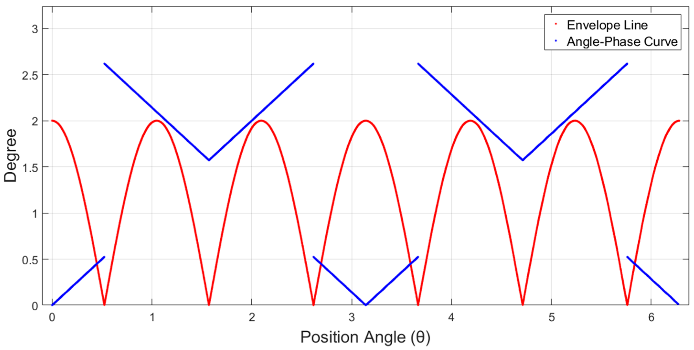
Figure 3 indicates the relations between stationary point and the switch of electrical angle in a BDFM with a set of 2-pole-pair stator power winding and a set of 4-pole-pair stator control winding. The x-coordinate indicates the position. The quasi-sinusoidal line is the envelope line, while the straight line is the corresponding electrical angle of each position. In Figure 3, the stationary point can be clearly seen. Every discontinuity point of this function corresponds precisely to the stationary point. Strictly speaking, the stationary point is not involved in the domain of this angle function, as on the stationary point, the dominator of the original form equals zero. This occasion just occurs when $k_{amp}=1$, while in other occasions the radical part of amplitude cannot reach zero. This phenomenon can be named as “stationary point switch”. It should be noticed that stationary point switch does not only happen in the occasion of $k_{amp}=1$, as this phenomenon is caused by the regular variance of released radical part:

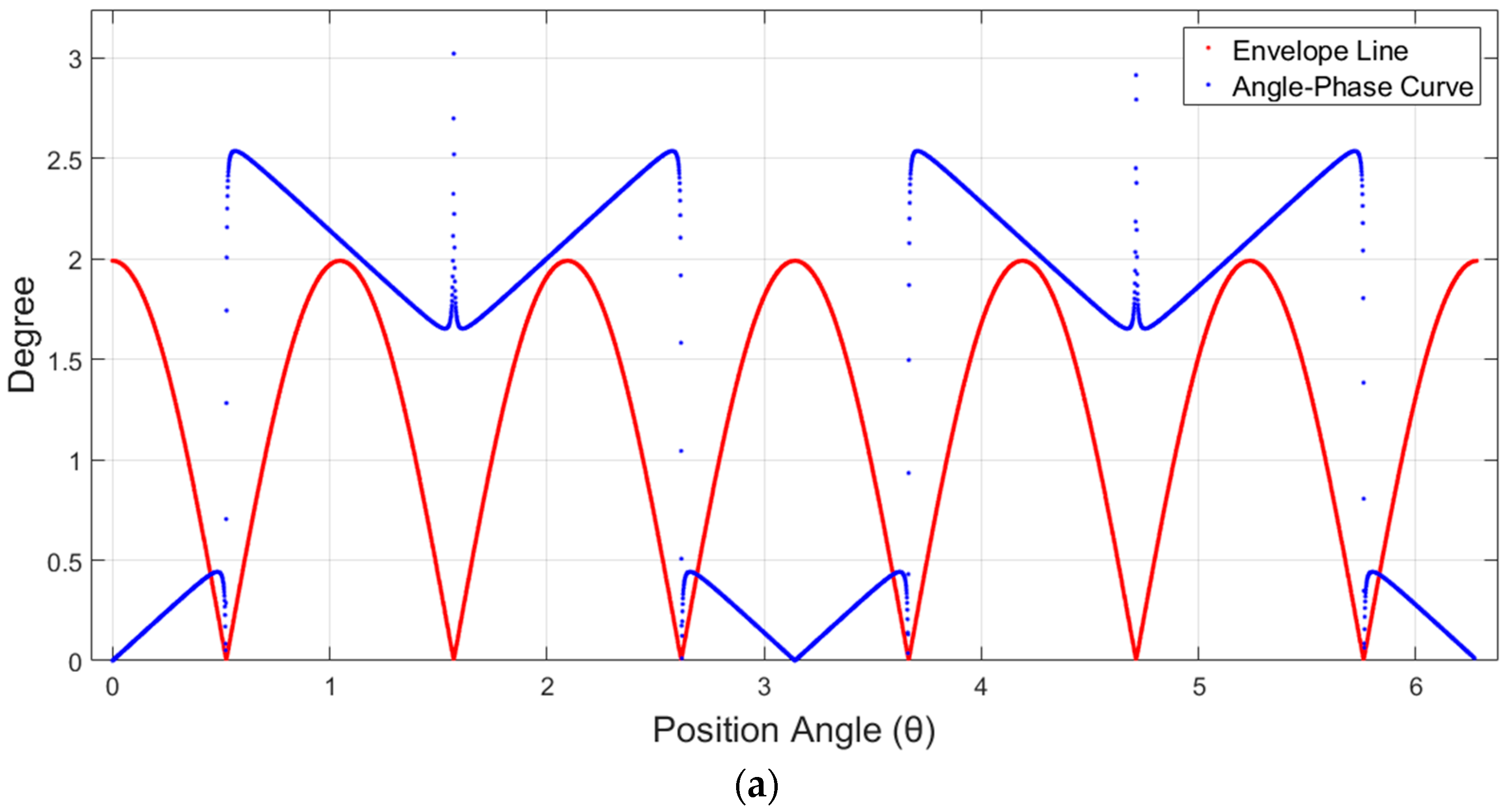
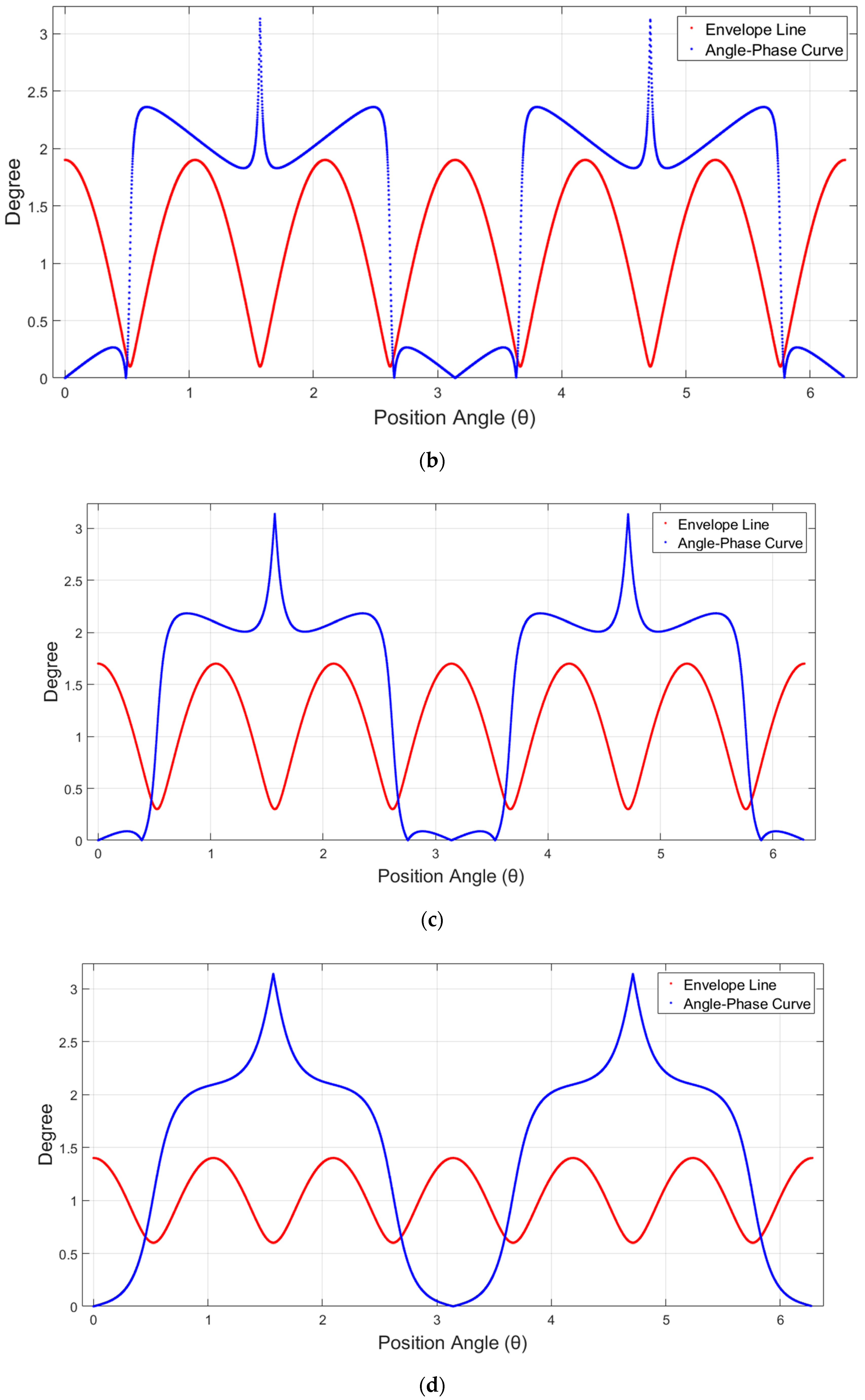
Four figures in Figure 4 lay out four different situations in which parameter $k_{amp}$ takes different values. The blue line indicates the situations of $k_{amp}<1$, while the red one stands for the envelope line in the corresponding $k_{amp}$. The analysis of this angle function indicates that this function is continuous when $k_{amp}<1$. Compared to the $k_{amp}=1$ situation, distortions in every position occur in all the other figures. When the amplitude gap between two magnetic potentials increases, the tendency of angle line distortion becomes more and more obvious. The variation of curve tends to shift close to the majority part of two components. When there is only one component left in the air gap, or the influence of the other one can be neglected in the air gap, the shape of the angle–position relation curve results:

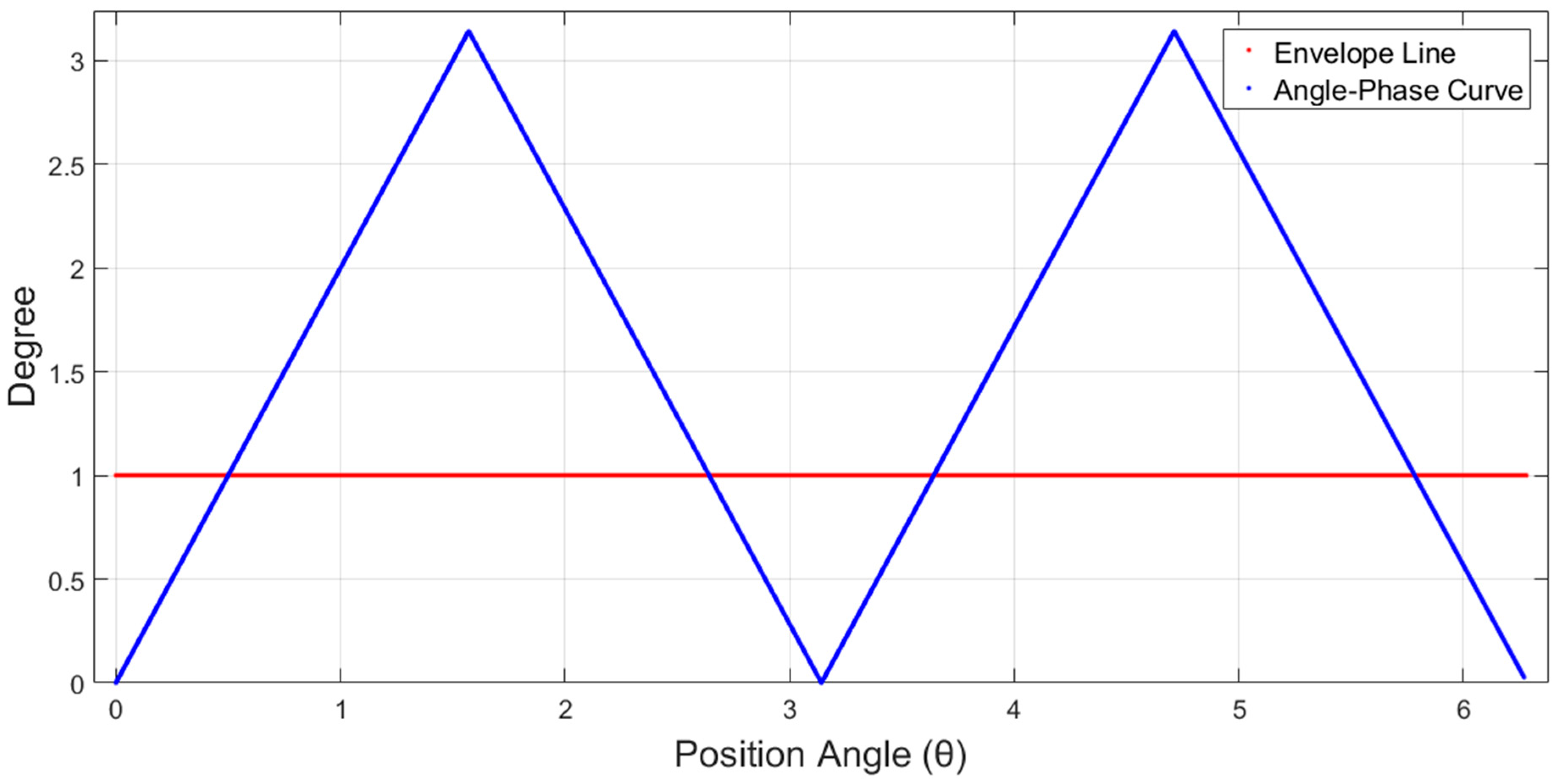
In Figure 5, there is only one magnetic field left in the air gap, thus, for every position on the rotor, the amplitudes of magnetic field stay the same, while the amplitude of each position occurs asynchronously. This is why the red line becomes a straight line, different from all the other figures.

The blue line in Figure 5 indicates the situation that only the control windings are left. Although this occasion rarely happens during the practical operation, it should not be ignored for theoretical research. From this figure, the relation between rotor position and electrical angle becomes quite clear and linear when the number of the magnetic field is one. The sum of triangle-sized shapes in each figure is decided by the number of pole pairs by counting the number of the triangle.

It should be pointed out that those situations mentioned above will become symmetrical when $k_{amp}$ takes the value of larger than 1. The tendency of the variation of angle–position relation will be close to the original relations of a 4-pole-pair shape as $k_{amp}$ tends to infinity, which is called the approximate situation of “only the field of power winding left in the air gap”.

Considering a normal working condition when the rotor of a single-frame BDFM rotates at a certain speed, the two sets of stator winding provide two different pole pair magnetic fields, which rotate at opposite directions if the coordinate system is set on the rotor side. Regardless how the speed varies, as long as the machine operates at a stable condition, the conclusions of standing-wave theory are always met. However, the existence of the harmonic wave and the winding coefficient restrictions during the machine design lead to the distortion of the standing wave. For almost all the occasions, the standard standing-wave curve is added by a small sinusoidal potential which leads to the offset of angle and amplitude variation. These formulas provide a detailed description of the fundamental wave of combined magnetic potential, and the corresponding relations between physical angle positions and electrical angles, while considering the offset, for a facultative moment of instantaneous value of the fundamental wave of magnetic potential, and the motive tendency of amplitude and electric angle can be predicted precisely, thus providing solid data of describing and observing the fundamental wave of BDFM.

4. Experimental Results

According to Faraday’s law, the variation of magnetic field would cause induced EMF in the conductor. Thus, the variation of magnetic field in one certain position can be observed by detecting the induced EMF of the measurement coil embedded in the rotor slot. As the measurement coils are embedded averagely in the rotor slot, the variation of the fundamental wave in the whole gap can be observed by analyzing the experimental data.

For a measurement coil, it would be useless if the two winding coefficients of induced power magnetic field and control magnetic field are not equal in the coil. The detailed distribution of air gap can be represented only when these two quantities scale at the same ratio.

Taking the influence of magnetic field induced by power windings into consideration, as an example, the induced voltage conducted by the field in an x-span measurement coil in the position ${\theta }_0$ can be expressed as:

$$sin\left(\omega t-p_p{\theta }_0\right)-sin\left[\omega t-p_p\left({\theta }_0+x\right)\right]$$

(16)

In the statement (16), all the other unrelated parts, such as the amplitude, integrations, and differentiations, are not displayed, and the coordinates are also set on the rotor. By using trigonometric transformation, the result can be expressed as follows:

$$2·cos\left[\omega t-p_p\left({\theta }_0+\frac{x}{2}\right)\right]·sin\left(\frac{p_p·x}{2}\right)$$

(17)

Thus from the control power side, the corresponding expression will be:

$$2·cos\left[\omega t+p_r\left({\theta }_0+\frac{x}{2}\right)\right]·sin\left(\frac{p_r·x}{2}\right)$$

(18)

As the aspect of amplitude has been swept out, the induction part holds the restrictive conditions of:

$$sin\left(\frac{p_p·x}{2}\right)=sin\left(\frac{p_r·x}{2}\right)$$

(19)

Obviously, $p_p$ is not equal to $p_r$ in the BDFM, thus the statement (19) can be rewritten as:

$$sin\left(\frac{p_p·x}{2}\right)=sin\left(\pi -\frac{p_r·x}{2}\right)$$

(20)

that is,

$$x=\frac{2\pi }{p_p+p_r}$$

(21)

$p_p+p_r$ indicates the number of the pole pair of rotor windings. From the view of the rotor side, a piece of measurement coil which owns a pitch of $2\pi /\left(p_p+p_r\right)$ can cover a whole single magnetic pole of combined magnetic field which is induced on the rotor. Moreover, the pitch of the coil ensures the ratio of the scaling of the two components stays the same, then the description of the distribution of the combined magnetic field can be derived by observing the induced electromotive force of measurements coils at different rotor positions.

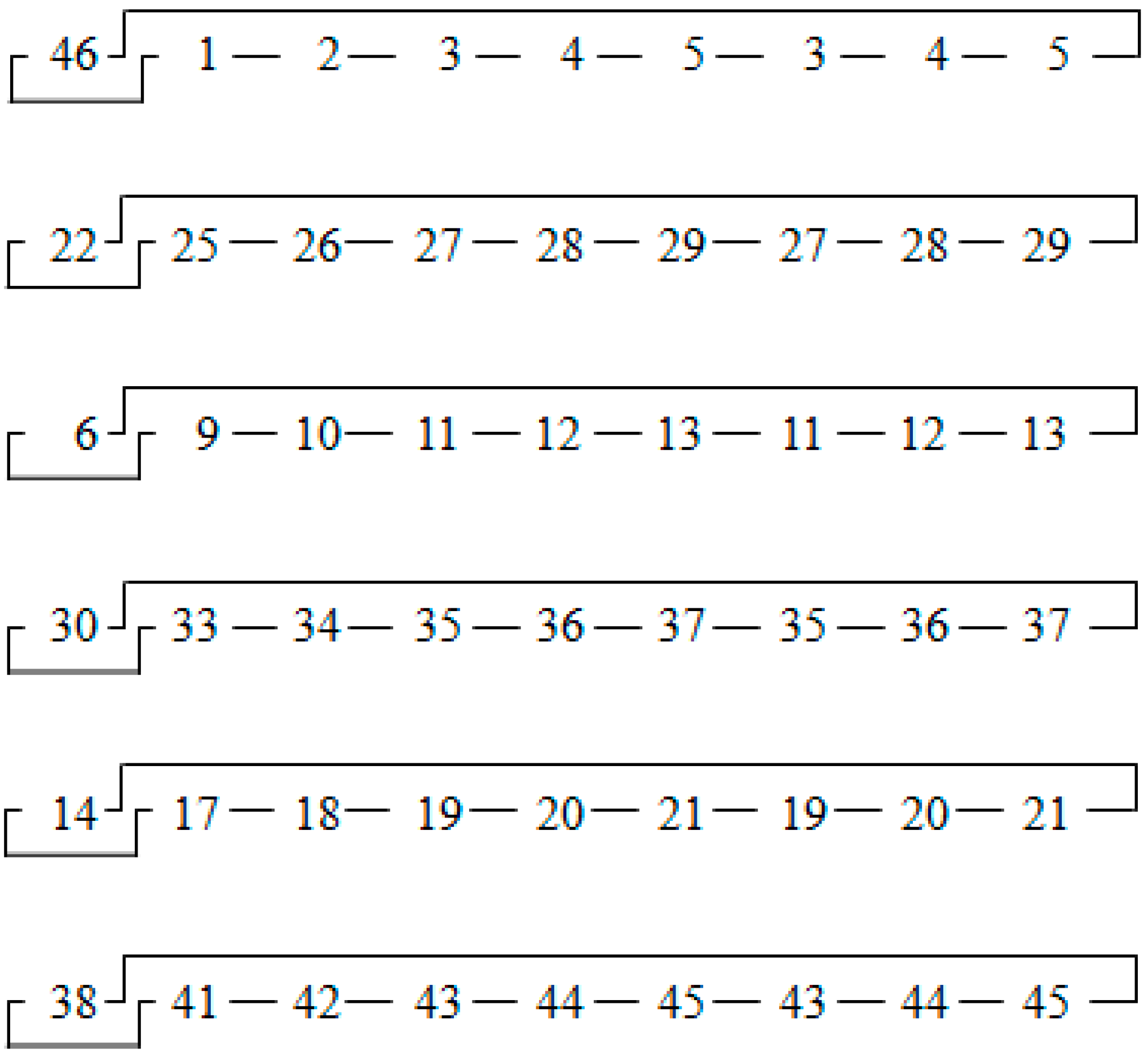
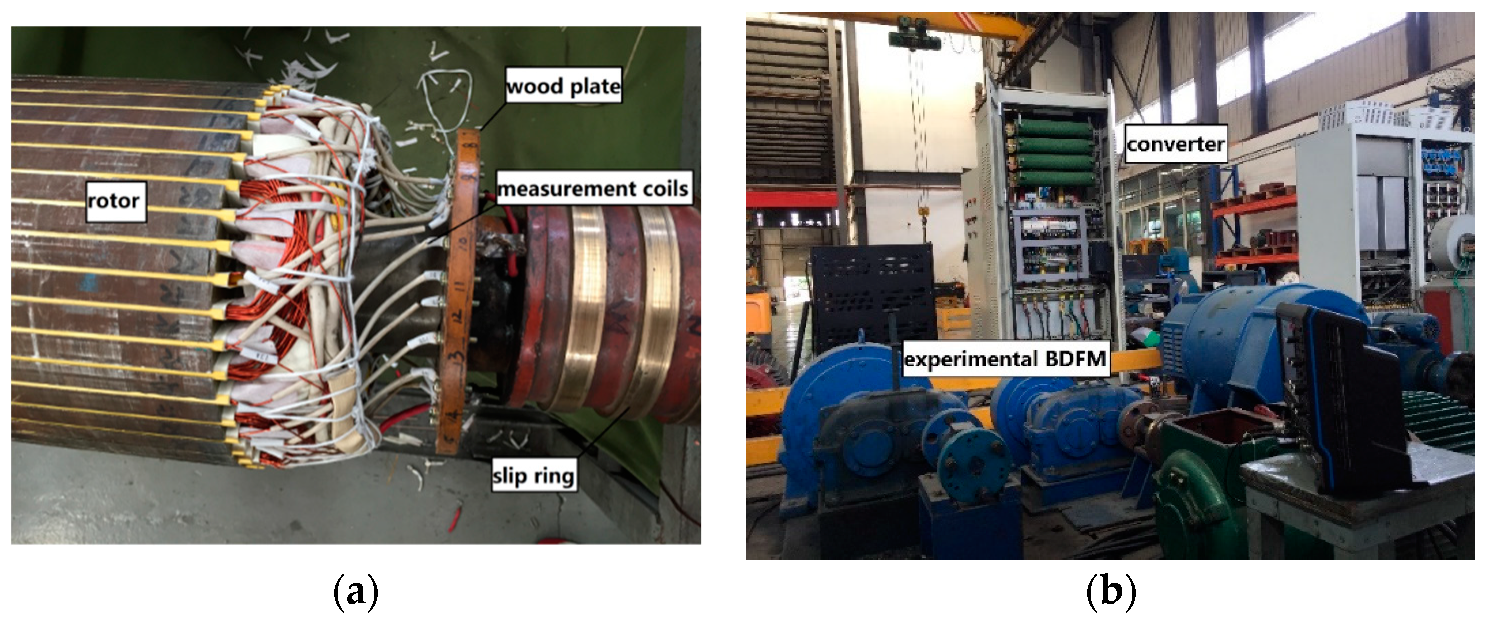
Figure 6 shows the structure of the prototype and the platform of the experiment. In order to give a detailed observation of air gap magnetic motive force (MMF), first, 24 measurement coils are set averagely in the rotor during the manufacturing process. By using a wood-made plate fixed on the rotor axis, all the 48 leads of these coils are connected to the plate in an isolated way. One coil as defined as a reference coil, and the upper-layer side of the reference coil is connected to one of the three slip ring terminals. Then, all the 24 under-layer sides of the coil are connected into another vacant terminal of a slip ring. The left slip ring terminal is connected to a removable, fixable wire lead. The other side of the lead is connected to one of the panel nodes of the 23 upper-layer sides of the measurement coils on the wood-made plate. Except the reference coil, all the other measurement coils are numbered and will be measured one by one during the experiment. Although the machine stops between every two consecutive measurements, the existence of the reference coil guarantees the relative electric angle relation between the chosen measurement coil and the reference coil, thus giving a support for drawing the electric angle relations figure.

During the measurement, 23 groups of data are recorded, while each group of data contains a measuring coil and the reference coil. By measuring and recording the amplitude, the relative angle position relations can be described. Each group of data demonstrates the variation of amplitude along with the time in a certain position. All the 23 groups of data are combined into one figure to which the x-coordinate contributes the rotor position. Thus, the combined figure becomes a discrete distribution.

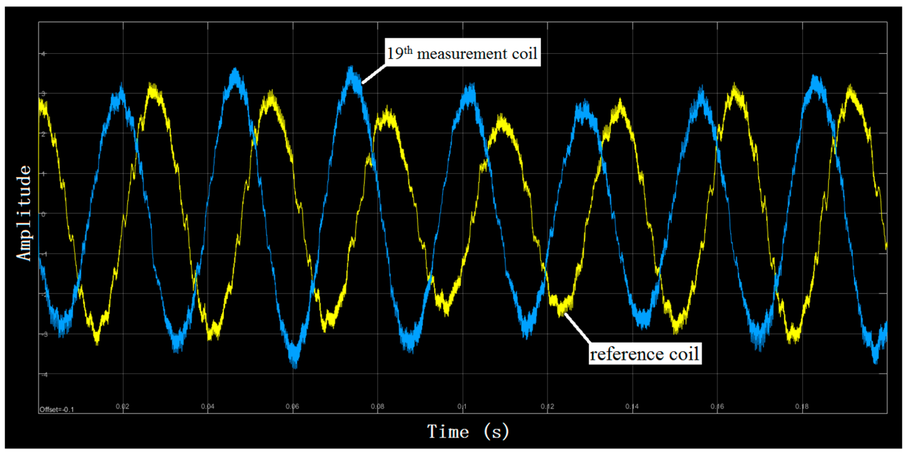
Figure 7 shows a 3k-filtered oscillograph of induced EMF in a certain measurement coil and the reference coil. The figure reveals the difference of induced EMF of two coils. With this figure, the tendency of variation in this position can be confirmed.

What should be pointed out is that Figure 7 displays the EMF amplitude variation of the 19th measurement coil as the time changes. If the representation of x-axis is changed to rotor position, all the data of the 19th measurement coil displayed in Figure 7 will be placed in a straight line, where the value of the x-axis represents the corresponding position of the rotor.

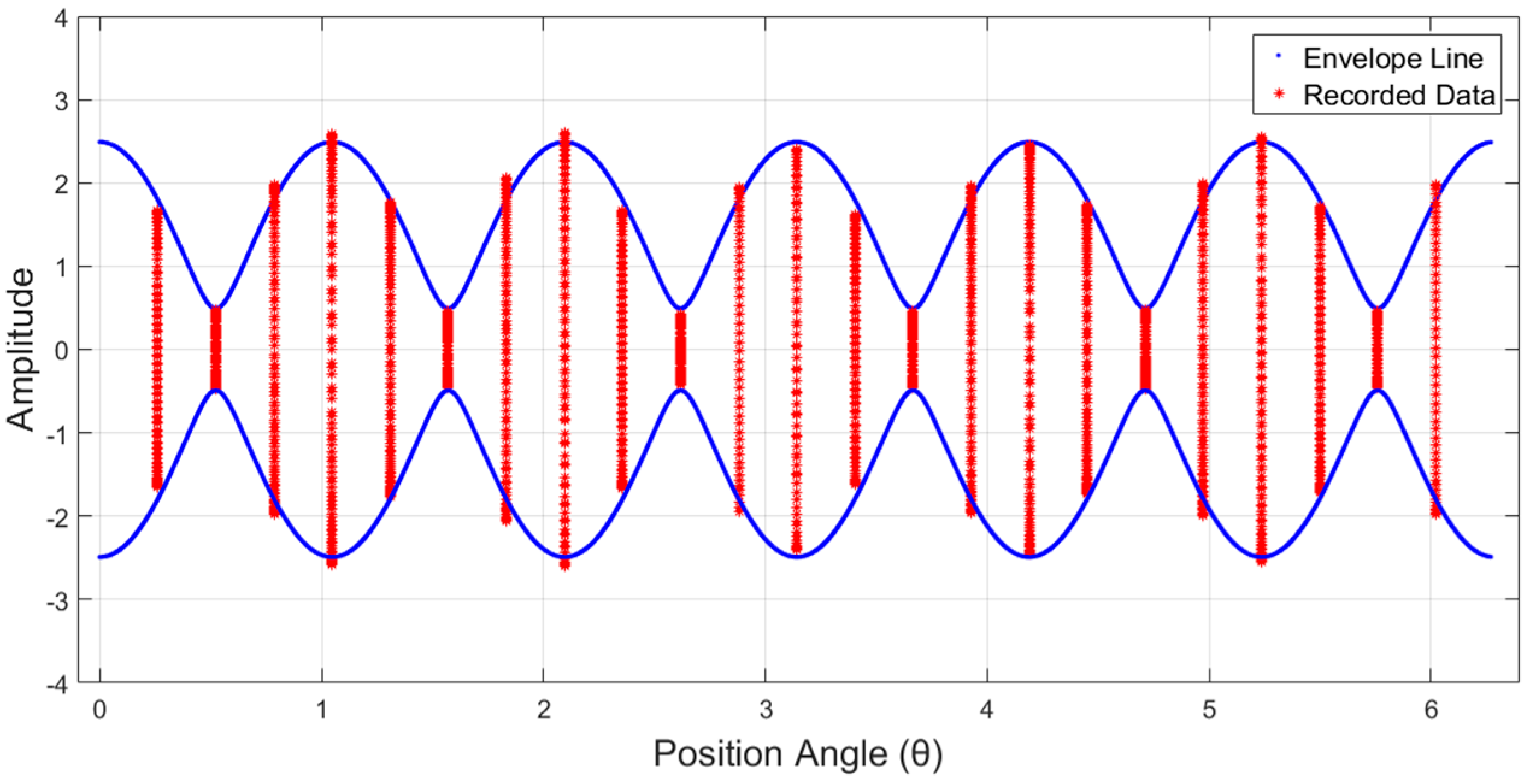
Figure 8 collects the data of all the 23 measurement coils, and all the data are placed according to their rotor position where they were recorded. Compared with Figure 7, which focuses on the regularity of value variation along with the time in one position, Figure 8 focuses on the regularity of value variation tendency in different positions of the whole rotor. By analyzing the range of data variation in different positions, some conclusions can be given.

In Figure 8, the x-axis represents the rotor positions, while the y-axis is for the corresponding value of induced EMF. This figure shows that each position has its own variation range of amplitude, which corresponds to the different magnetic field density. As the amplitudes of two stator magnetic fields do not equal the same, the minimum of induced EMF does not reach zero, just as the blue line reveals. From the figure data, the two amplitudes of induced EMF can be calculated as 1.67 and 1.12. According to this data, the envelope line of this combined field can be drawn out. The ratio of two fields is $1.12/1.67=0.671$, while the corresponding value based on

Table 1. Configuration parameters of experimental wound-rotor BDFM.

Parameters	Value	Parameters	Value
Rated voltage (V)	380	Rated power (k)W	10
Range of Power Winding Current (A)	0–20	Range of Control Winding Current (A)	0–20
Number of stator slot	72	Number of rotor slot	48
Pole pair of power windings	4	Pole pair of control windings	8
External diameter of stator (mm)	368	External diameter of rotor (mm)	280
Interior diameter of stator (mm)	280	Interior diameter of rotor (mm)	100
Length of stator core	28	Number of mea. coils 1	23
Number of turns per mea. coils	1	Mea. coil pitch	16
Winding coefficient of rotor power side	0.595	Winding coefficient of rotor control side	0.795

¹ Mea. calls for word ‘measurement’.

is 0.6681, quite close to the experimental value.

In the experiment, the rotor speed is 400 rpm, which means the frequency of the rotor field equals $110/3 \mathrm{Hz}$. From Figure 7, two expressions of measurement coil and reference coil can be written down. The expressions focus on its amplitude and initial phase angle. However, as the recording moments of 23 coils are facultative, it is not necessary to observe the 23 coils by ignoring the corresponding situations on the reference coil.

Table 2. Expressions of 23 groups of coils and corresponding phase separations.

Measurement Coil Number	Expressions of Measurement Coil	Expressions of Reference Coil	Phase Separations
1	$1.66076·cos\left(220/3·\pi t+0.48027\pi \right)$	$2.59582·cos\left(220/3·\pi t+0.44498\pi \right)$	$+0.0353\pi$
2	$0.47639·cos\left(220/3·\pi t-0.96317\pi \right)$	$2.55593·cos\left(220/3·\pi t-0.46297\pi \right)$	$-0.5002\pi$
3	$1.98764·cos\left(220/3·\pi t+0.28566\pi \right)$	$2.66803·cos\left(220/3·\pi t-0.99840\pi \right)$	$+1.2841\pi$
4	$2.58651·cos\left(220/3·\pi t-0.05220\pi \right)$	$2.51833·cos\left(220/3·\pi t+0.61736\pi \right)$	$-0.6696\pi$
5	$1.76316·cos\left(220/3·\pi t+0.92633\pi \right)$	$2.54717·cos\left(220/3·\pi t-0.44202\pi \right)$	$+1.3684\pi$
6	$0.46136·cos\left(220/3·\pi t+0.25763\pi \right)$	$2.53706·cos\left(220/3·\pi t-0.56633\pi \right)$	$+0.8240\pi$
7	$2.06759·cos\left(220/3·\pi t+0.11740\pi \right)$	$2.58683·cos\left(220/3·\pi t-0.50101\pi \right)$	$+0.6184\pi$
8	$2.60331·cos\left(220/3·\pi t-0.82090\pi \right)$	$2.55604·cos\left(220/3·\pi t+0.52453\pi \right)$	$-1.3454\pi$
9	$1.66594·cos\left(220/3·\pi t-0.13007\pi \right)$	$2.39395·cos\left(220/3·\pi t+0.56282\pi \right)$	$-0.6929\pi$
10	$0.43207·cos\left(220/3·\pi t-0.64617\pi \right)$	$2.36903·cos\left(220/3·\pi t-0.46693\pi \right)$	$-0.1792\pi$
11	$1.95314·cos\left(220/3·\pi t-0.93439\pi \right)$	$2.47039·cos\left(220/3·\pi t-0.96703\pi \right)$	$+0.0326\pi$
12	$2.40383·cos\left(220/3·\pi t-0.64561\pi \right)$	$2.33488·cos\left(220/3·\pi t-0.63899\pi \right)$	$-0.0066\pi$
13	$1.61669·cos\left(220/3·\pi t-0.45806\pi \right)$	$2.36316·cos\left(220/3·\pi t-0.41098\pi \right)$	$-0.0471\pi$
14	$0.45339·cos\left(220/3·\pi t-0.34831\pi \right)$	$2.43916·cos\left(220/3·\pi t-0.87015\pi \right)$	$+0.5218\pi$
15	$1.96754·cos\left(220/3·\pi t+0.96434\pi \right)$	$2.46276·cos\left(220/3·\pi t+0.24471\pi \right)$	$+0.7196\pi$
16	$2.45088·cos\left(220/3·\pi t+0.29088\pi \right)$	$2.37083·cos\left(220/3·\pi t-0.36587\pi \right)$	$+0.6568\pi$
17	$1.72798·cos\left(220/3·\pi t-0.15299\pi \right)$	$2.49358·cos\left(220/3·\pi t+0.47075\pi \right)$	$-0.6237\pi$
18	$0.47836·cos\left(220/3·\pi t-0.07241\pi \right)$	$2.58484·cos\left(220/3·\pi t-0.92141\pi \right)$	$+0.8490\pi$
19	$1.99905·cos\left(220/3·\pi t-0.00218\pi \right)$	$2.61969·cos\left(220/3·\pi t-0.61098\pi \right)$	$+0.6089\pi$
20	$2.55375·cos\left(220/3·\pi t+0.80405\pi \right)$	$2.60210·cos\left(220/3·\pi t+0.12892\pi \right)$	$+0.6751\pi$
21	$1.71709·cos\left(220/3·\pi t+0.15235\pi \right)$	$2.50979·cos\left(220/3·\pi t-0.53929\pi \right)$	$+0.6916\pi$
22	$0.46144·co\mathrm{s}\left(220/3·\pi t-0.41867\pi \right)$	$2.56607·cos\left(220/3·\pi t-0.60420\pi \right)$	$+0.1855\pi$
23	$1.97756·cos\left(220/3·\pi t-0.35216\pi \right)$	$2.56851·cos\left(220/3·\pi t-0.30794\pi \right)$	$-0.0422\pi$

lays out the original expressions of 23 groups of coils and their phase separation. Compared to the statement (12), the phase separation needs a bit of transformation, as the range of arc cosine functions cover from 0 to $\pi$.

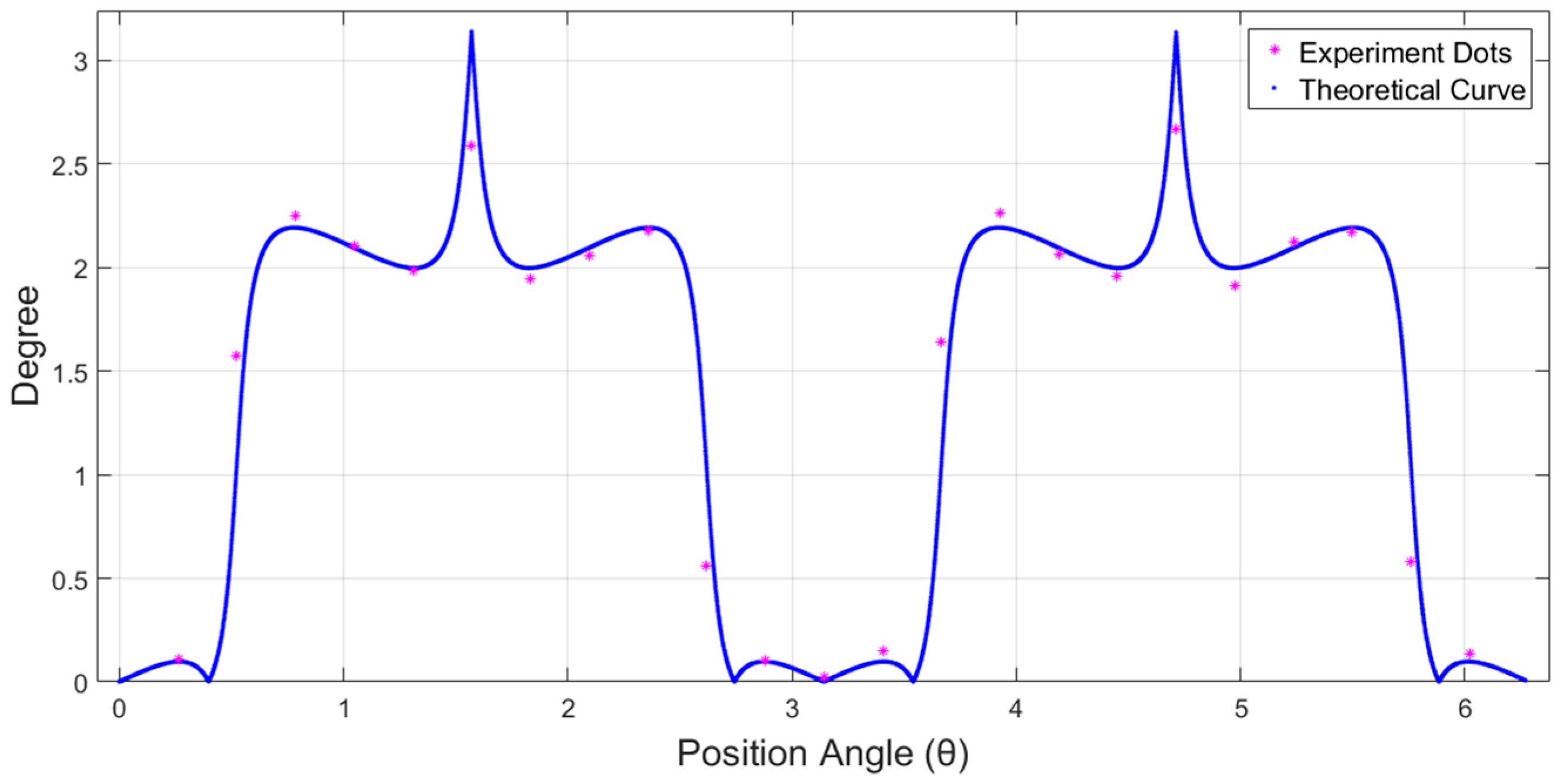
The blue line in Figure 9 is the theoretical angle–position relation when the amplitude ratio of two magnetic fields $k_{amp}$ equals 0.67, which is the same as the calculated result. The pink dots in the same figure are the processed phase separations of 23 different rotor positions, while these separations are all based on the restrictions of “the initial angle of reference coil always remains zero”, that is, the comparison standard has been united to one coil, which is the reason why every record calls for the measurement of the reference coil. In Figure 9, the angle separations based on the same reference coil are placed on the figure, and are quite close to the theoretical line by using the calculated $k_{amp}$ value. The errors in the figure are mostly caused by sampling and recording.

5. Conclusions

This paper provides a detailed expression of the fundamental wave of the magnetic field in the air gap. The fundamental wave reveals a standing wave form when it is observed from the rotor side. Due to the restriction of mechanical design, in many situations, the amplitude ratio cannot be set as a theoretical value, which leads to the distortion of the combined field and the distortion can be demonstrated by the enveloping line of the fundamental wave of the rotor field.

Also, the relations between rotor position and rotor angle are quite different from the traditional electrical machine due to the special structure and the combination of magnetic fields. The rapid variation of rotor angle is closely related with the stationary points on the rotor field.

Finally, a prototype wound-rotor BDFM is manufactured with 23 measurement coils. By detecting and analyzing the recorded data, the enveloping line of the fundamental wave of the magnetic fields can be described, and the relations between the rotor angle and its position are verified.

The detailed expression is helpful for studying principles of wound-rotor BDFMs and determining the basic characteristics of the fundamental wave in the air gap of the machine, which provides the reference on the rotor design of BDFMs. However, the effects of saturation and the slotting are neglected in the discussion.