Integration of Flow Temperatures in Unit Commitment Models of Future District Heating Systems

Abstract

The transformation of heat supply structures towards 4th generation district heating (4GDH) involves lower supply temperatures and a shift in technology. In order to assess the economic viability of the respective systems, adequate unit commitment models are needed. However, maintaining the formal requirements, while reducing the computational efforts of these models, often includes simplifications such as the assumption of constant supply temperatures. This study investigates the effect of introducing varying supply temperatures in mixed-integer linear programming models. Based on a case study of a municipal district heating system, how the temperature integration approach affects unit commitment and technology assessment for different temperature levels and scenarios is analyzed. In particular, three supply temperature levels are investigated with both variable and constant temperatures in two scenarios. Results indicate that lower flow temperature levels in the heating network tend to favor internal combustion engines, combined cycle power plants, and heat pumps; while back pressure steam turbines, peak loads, and electric boilers show declining operating hours. Furthermore, the effect of varying versus constant temperatures at the same temperature level is rather small, at least as long as technical restrictions do not come into play. Finally, it is found that the effect of changing temperature on a technology assessment is comparably small as opposed to adaptions in the regulatory framework.

1. Introduction

District heating (DH) systems can play a central role in decarbonizing energy systems, as they can provide flexibility within the electricity and heat sector. For these systems, the concept of 4th generation district heating (4GDH) has been developed [1]. Besides a combination of different and flexible heating technologies, low supply temperatures are an important part of such systems to increase overall energy efficiency.

An assessment of economic viability for these systems requires adequate methods. For this purpose, often linear programming (LP) or mixed-integer linear programming (MILP) models are applied [2]. Operational results are evaluated from a technical, economic, or environmental perspective to identify suitable technologies, plant setups, or energy infrastructure designs. However, models must include simplifications to retain their formal requirements and reduce computational efforts. One of these simplifications is the assumption of constant flow temperatures, although in practice temperatures vary for a given heating system due to the heat load, weather conditions, and other external factors.

This study investigates the integration of varying supply temperatures in MILP models of DH systems along three main research questions:

• How can varying temperatures be integrated in linear optimization models of future DH systems?
• How does the flow temperature level influence the operational results?
• How significant are the deviations between results modeled with varying and constant temperatures?

To answer these questions, a respective techno-economic operational optimization model is described in detail and applied in a case study of a heating plant. Two different economic scenarios are considered and the effects of three different temperature levels (low, medium, and high) within the network is studied. The heat load is modeled with both variable and constant supply temperatures. Based on this, cost-optimal solutions and optimized operation schedules are compared and analyzed.

2. State of Research and Scientific Contribution

There are several analytical approaches for modeling DH systems with constant flow temperatures. In Reference [3] an MILP approach is used to analyze the contribution of thermal energy storage (TES) in liberalized electricity markets. A similar approach is applied in Reference [4] to design small scale distributed energy systems based on a multi-criteria method; by evaluating investment and operational costs as well as operational CO₂ emissions. A stochastic programming approach to address parametric uncertainty considering a broad range of technologies such as extraction turbines, peak load boilers (PLB), and TES can be found in Reference [5]. Other models include distributed combined heat and power generation in virtual power plants [6], the assessment of TES in centralized systems [7], and the analysis of DH systems in renewable energy-based power systems [8]. Although all of these models differ with respect to their research questions, many mathematical formulations are similar for the modeled components [2].

For models with constant flow temperatures the impact of model simplifications in terms of the accuracy of the results has been assessed by Reference [9]. This investigation compares LP, MILP, and non-linear programming (NL) approaches and concludes that MILP approaches are well suited for coping with the trade-off between runtime and accuracy.

However, supply temperatures vary due to weather conditions and demand patterns throughout the year and, in combination with the absolute heat load, therefore are an integral characteristic of the heating system. The efficiency and the operational restrictions of heat technologies are affected by this to a varying extent. The efficiency of a PLB only varies in the range of a few percent [10], whereas the coefficient of performance (COP) of heat pumps (HP) is significantly influenced by the source and sink temperature.

Nevertheless, only a few papers describe models with variable flow temperatures. To assess the potential of HP in the Copenhagen heating network, a model for HP with varying COP is applied in Reference [11]. The study shows that different temperature levels in the transmission and the distribution network may have a significant impact on the operation of the HP due to the temperature dependence of the COP. The study results imply that for certain technologies such as HP, the flow temperature representation is crucial for an adequate system assessment. To our knowledge, the influence of varying supply temperatures and their effect on the unit commitment and the economic assessment of multi-technology systems has not been studied so far.

This paper broadens the current state of research by investigating the assumption of varying versus constant flow temperatures in (mixed-integer) linear programming models for a broad set of typical DH technologies and different temperature levels. In contrast to other studies, it specifically analyzes how the temperature integration approach affects the unit commitment and the resulting technology assessment.The results derived here can be relevant for future studies in which an adequate modeling approach for different technologies and temperature setups has to be chosen.

3. Model Description

To investigate the impact of varying flow temperatures in multi-technology DH systems, an MILP unit commitment model has been developed. The model optimizes the operational profit of the overall plant with respect to the technical restrictions of the represented technologies under the assumption of perfect foresight. For the implementation, the open source Open Energy Modelling Framework (oemof) was chosen [12].

3.1. General Overview

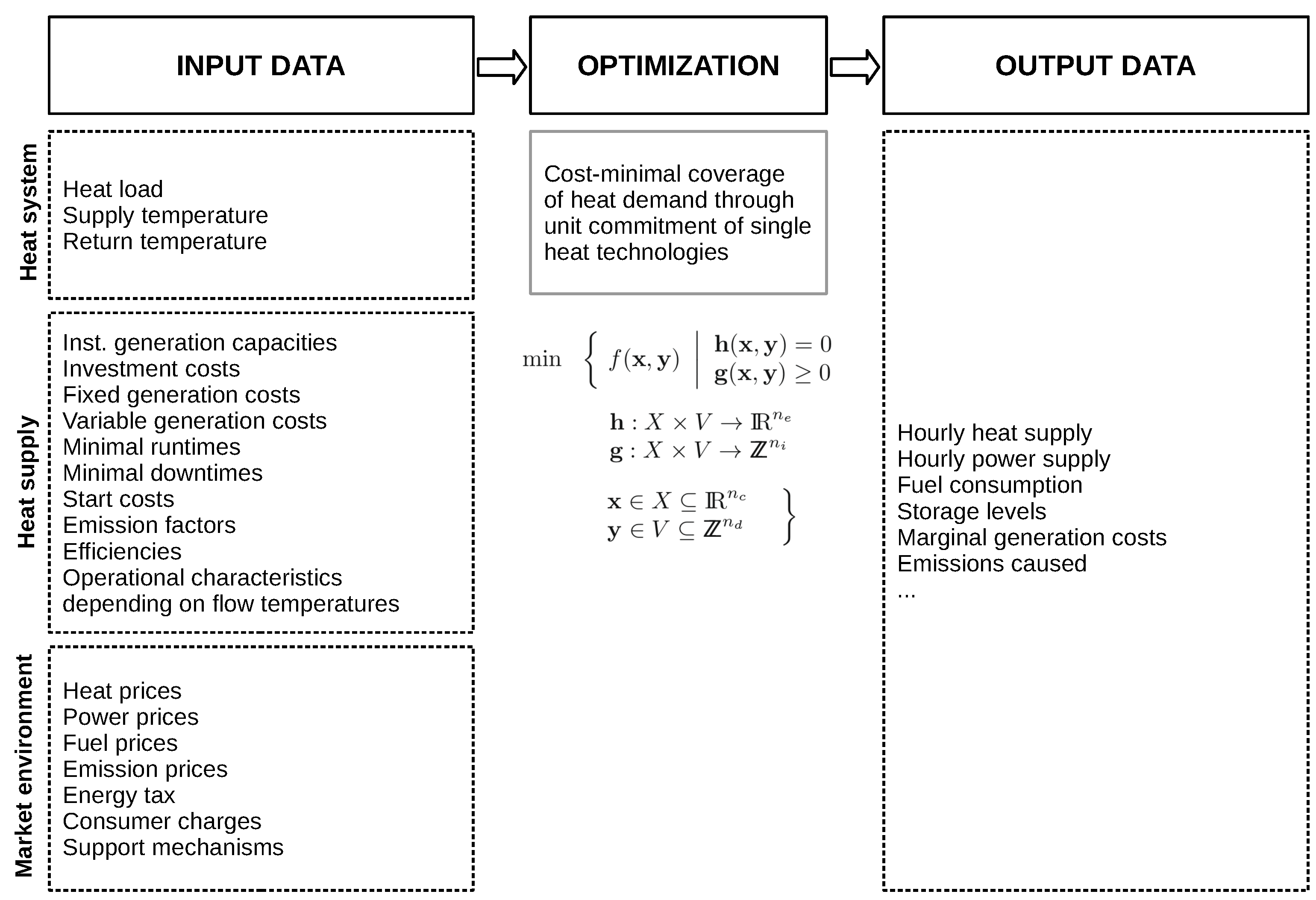
Figure 1 shows the model with all of the relevant input parameters and decision variables. The DH network is not modeled based on its detailed physical characteristics such as flows, losses, or pumping. Instead, the heat demand is given as an hourly load profile at the plant site. Supply temperatures are exogenous model parameters and can either be constant or fluctuating over time. Due to minor variations compared to the supply temperature conditions, the return temperature is set at a constant value. This assumption may have to be revised if the impact of the variable supply temperature integration proves to be significant.

Similarly, the electric grid is not included in the model, so that additional restrictions such as an electricity balance within the supply system are not considered. Market prices for heat, electricity, and fuel are represented as time series in hourly resolution. Furthermore, the market environment is able to incorporate regulatory measures such as emission certificates, energy taxes, electricity consumer charges, and the combined heat and power (CHP) support mechanisms. Based on the input data provided, the model computes the supply and demand of heat and electricity for the individual DH technologies involved, as well as the storage levels if applicable. In combination with the input data, economic indicators such as profits are calculated.

3.2. Technology Representation

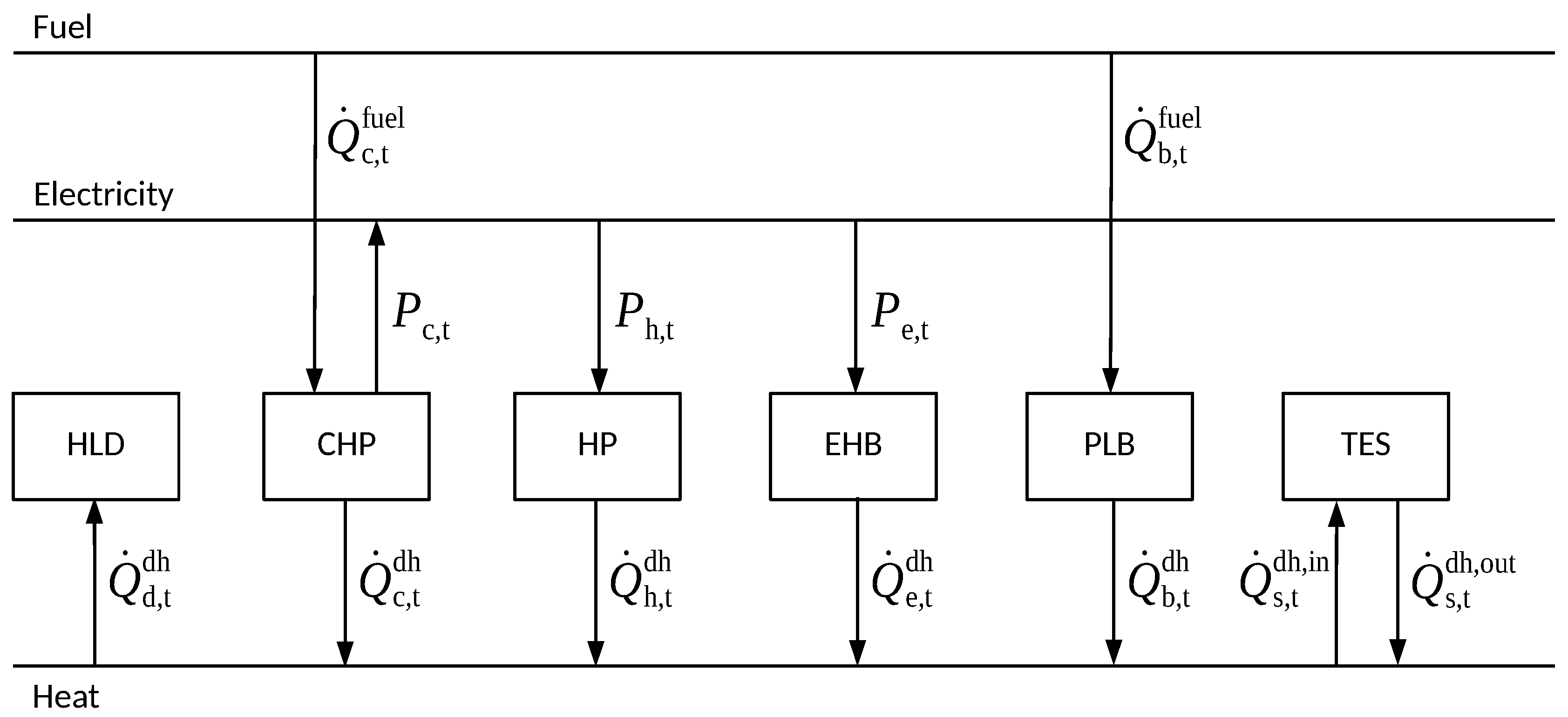
As illustrated in Figure 2, the given heat load (HLD) is to be met by a plant setup. This plant potentially consists of combined heat and power plant (CHP) technologies, power to heat (PTH) technologies—here depicted separately as HP and EHB (electric heating boiler) due to different modeling formulations—as well as PLB and TES. Subsequently, characteristics for these technologies are described in a parallel setup.

Whereas some technology characteristics can be expressed as fixed or feed flow independent parameters, others vary with supply temperature conditions. The former group includes installed capacities and related investment costs, fixed and variable operating costs, minimum runtimes, and minimum downtimes. In addition, feed flow independent but market-related figures such as fuel costs, start costs, and emission factors for fuel and electricity consumption are determined for each time step and collectively summarized in a sequence. Further characteristics indicate the operational behavior including representations of the efficiency, maximum and minimum extractable heat or power, and other operational restrictions. These figures especially react to varying supply temperatures. However, the extent to which the figures are affected by varying flow temperatures depends strongly on the technology type and layout.

3.2.1. Combined Heat and Power

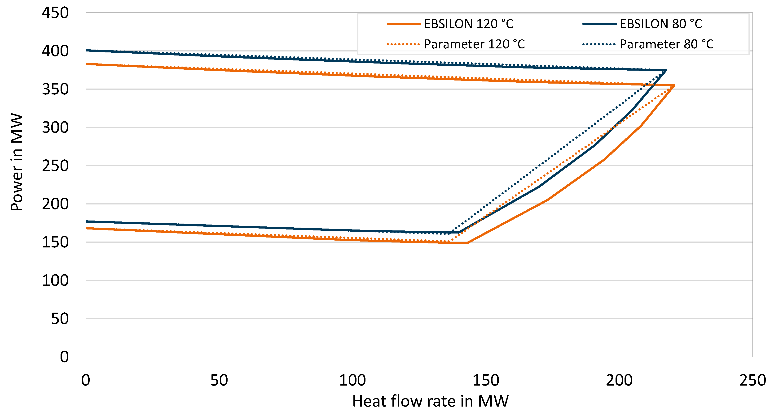
Internal combustion engines (ICE), back pressure steam turbines (BPT), and combined cycle power plants with extraction steam turbines (CET) are grouped as CHP technologies. These exploit fuel resources to provide heat and power to the respective systems. With shifting supply temperatures and loads, the technologies show strong variations in their efficiency and operational restrictions [13,14,15]. This effect is shown in Figure 3 for two different supply temperatures. The feasible operational range, in terms of simultaneously extractable heat and power, has been calculated for an exemplary CET plant with supply temperatures of 80 ${}^{\circ }$C and 120 ${}^{\circ }$C using the EBSILON software [16]. Upper and lower bounds for the supply temperature are related to the constant maximum and minimum fuel supply, respectively. A necessary minimum mass flow in the last turbine stage limits the heat extraction with varying fuel supply, indicated by the right boundary. The P–$\dot{Q}$-diagram shows that lower supply temperatures lead to higher feasible power, while the heat supply and fuel consumption remain constant, thus causing higher efficiencies and a lower maximum heat supply.

As Reference [17] states, any CHP system can be modeled by the irregular quadrilateral shape of the operational range in a P–$\dot{Q}$-diagram. This approach, as it is also applied similarly in Reference [18,19], is used for modeling CHP technologies and extended by a restriction limiting the minimum extractable heat flow in case of an ICE. The dotted lines in Figure 3 indicate the operational boundaries linearized by a set of equations and inequalities using technology and supply temperature-specific variables. These variables are used in the optimization, as pre-calculated hourly sequences, which in turn are derived from a supply temperature dependent linear function. An example case is shown in Equation (1) for the maximum providable power without heat extraction of the CET.

$$\begin{array}{cc}\hfill {\overline{P}}_{c,t}^{wodh}& =m_c{T}_t^{st}+b_c\forall c.\hfill \end{array}$$

(1)

3.2.2. Power to Heat

PTH plants convert electric energy into heat and can provide additional flexibility in the electricity system. The two respective technologies considered in the optimization model, EHB and HP, exhibit completely different operating principles and hence have to be modeled differently. EHB are based on electrodes, which heat up water through direct heat transfer. Therefore, EHB show an almost constant efficiency over their operating range even when heat loads and supply temperatures vary. Consequently, the general approach is to model an EHB with a supply temperature independent, power to heat conversion variable, as applied in References [9,20,21]. This is also implemented here.

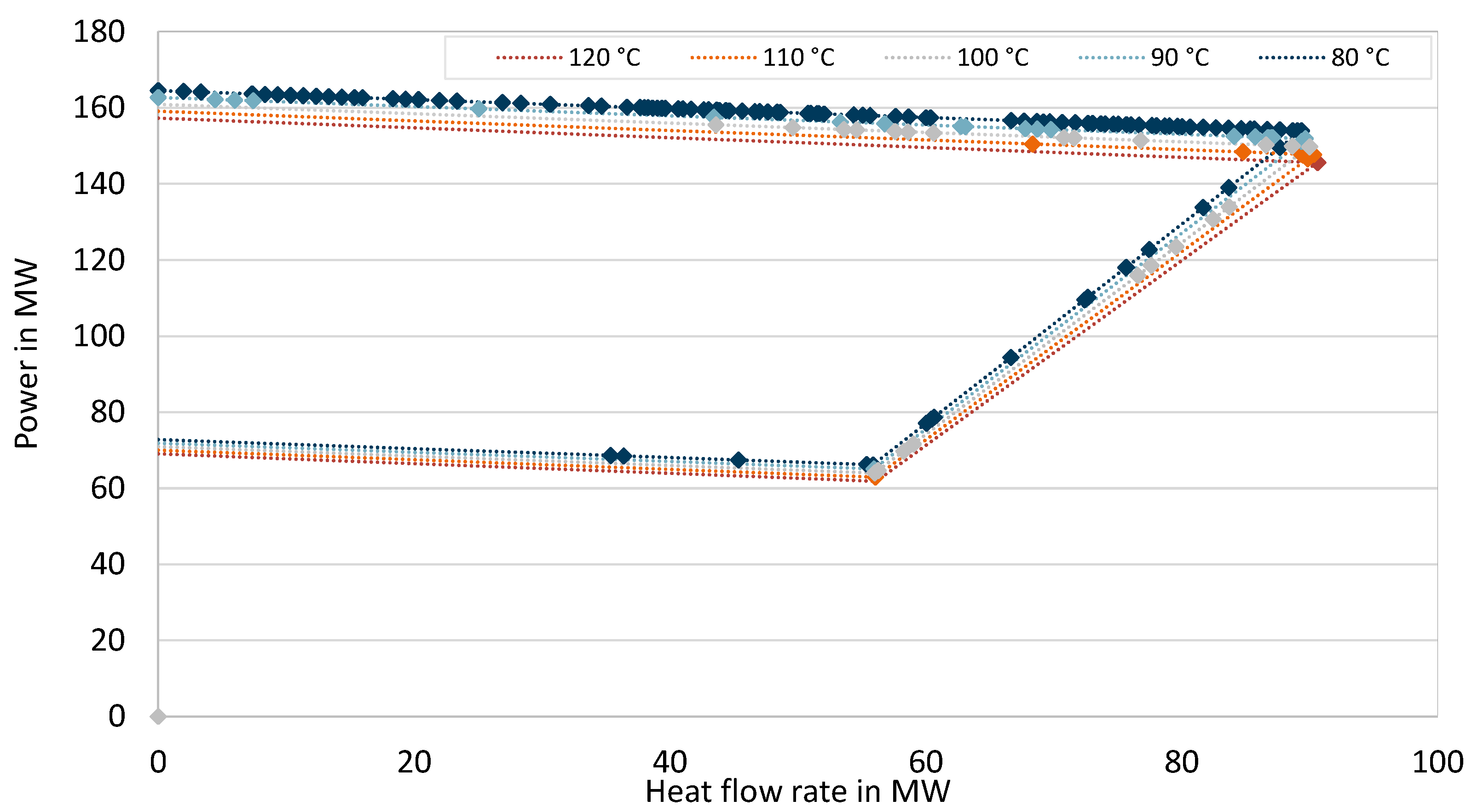
HPs convert heat from a low temperature level into heat at a usable high temperature level by adding electric energy. Varying sink and source temperatures as well as fluctuating heat loads have a considerable influence on the HP efficiency, in terms of the COP, and on operational restrictions [22]. In this context, a detailed model of an HP, that includes the dependencies of the COP and operational restrictions, with supply temperature variations is proposed. Assuming a constant source temperature, ensured by a geothermal heat source, a linear function with supply temperature specific variables relates the necessary power input to the retrieved heat output. In addition, temperature specific minimum and maximum heat loads are introduced. Similar to the CHP formulation, these variables have to be pre-calculated by supply temperature dependent linear functions retrieved from HP simulations by EBSILON. Equation (2) expresses this model in terms of the slope of the heat–power function of Equation (23).

$$\begin{array}{cc}\hfill {ϵ}_{h,t}^m& =m_h{T}_t^{st}+b_h\forall h.\hfill \end{array}$$

(2)

3.2.3. Thermal Energy Storage

In heating systems, the production flexibility is increased by the integration of TES. Amongst others, pressurized water tanks as sensible for TES, and are often used for this purpose. Variable supply and return temperatures, in addition to heat losses, lead to temperature stratification effects in the TES. This makes TES technology a complex component in plant modeling, as storage content and feasible supply temperature are a function of the thickness of temperature layers. Many different approaches can therefore be found in literature so far. Most studies model the TES with constant inlet and outlet temperatures without considering losses, thus determining a simple two zone temperature representation of the stored energy as a function of the entering and exiting energy or mass flows [3,4,5]. Additionally, energetic losses can be considered while still keeping relevant temperatures constant [6,23,24]. In other modeling problems, the TES is often discretized into many horizontal layers for a more detailed representation. However, this formulation increases the computational complexity leading to its rare application in optimization models. For this reason, a simplified TES model with storage content related to energy inflows and outflows, and neglecting stratification effects is applied. Generally, further analysis on different TES technologies with related appropriate mapping methods is required, which is not focus of this paper.

3.2.4. Peak Load Boiler

PLBs fired with conventional primary resources or biomass usually complement heating plants to meet peak load demands. In praxis, efficiency variations of 3 to 5% are determined with variable supply temperatures and load variations within the feasible range [9,10]. In several studies, this behavior is either simplified by a constant efficiency [4,6,8] or depicted as a linear function of the heat load [25] in a certain operating range. Because of the minimal performance variation, the efficiency is subsequently assumed as constant.

3.3. Formulation as a Mixed-Integer Linear Program

An overview of the employed identifiers, symbols, and index sets is provided in the nomenclature at the end of the paper. Identifiers are used to specify variables and parameters in the model description. The formulation of sets holds for any number of technologies that is contained in a specific set and an arbitrary number of time steps. Subsets and empty sets, for the case of non-existent units, are thus also covered.

The objective function in its general form is described in Equation (3) using the described identifiers, indices, and sets. It consists of single expressions for costs and revenues that are related to single technologies, which are explained in Equations (4)–(11). Costs for CHP units are described in Equation (4) and consist of fuel prices, costs for CO₂ certificates, variable costs of electricity generation, and fuel-dependent start costs. In contrast, all revenues for delivered heat and power are expressed in Equation (5). Costs and revenues for other technologies are expressed in the same way and are always related to the specific input and output quantities. If not mentioned explicitly, all (non-heat) capacities are assumed to be electrical capacities in the following.

$$\begin{array}{cc}\hfill min& [{\displaystyle \sum _t}({\displaystyle \sum _c}(C_{c,t}-R_{c,t})+{\displaystyle \sum _h}(C_{h,t}-R_{h,t})\hfill \\ & +{\displaystyle \sum _e}(C_{e,t}-R_{e,t})+{\displaystyle \sum _b}(C_{b,t}-R_{b,t}))]\hfill \end{array}$$

(3)

$$\begin{array}{cc}\hfill C_{c,t}& ={\dot{Q}}_{c,t}^{fuel}\tau (c_{c,t}^{fuel}+c_t^{emi})+P_{c,t}\tau c_{c,t}^{var}+Y_{c,t}^{start}{c}_{c,t}^{start}\hfill \end{array}$$

(4)

$$\begin{array}{cc}\hfill R_{c,t}& ={\dot{Q}}_{c,t}^{dh}\tau c_t^{dh}+P_{c,t}\tau c_t^{elm}\hfill \end{array}$$

(5)

$$\begin{array}{cc}\hfill C_{h,t}& =P_{h,t}\tau (c_t^{elm}+c_{h,t}^{var})+Y_{h,t}^{start}{c}_{h,t}^{start}\hfill \end{array}$$

(6)

$$\begin{array}{cc}\hfill R_{h,t}& ={\dot{Q}}_{h,t}^{dh}\tau c_t^{dh}\hfill \end{array}$$

(7)

$$\begin{array}{cc}\hfill C_{e,t}& =P_{e,t}\tau c_t^{elm}+{\dot{Q}}_{e,t}^{dh}\tau c_{e,t}^{var}+Y_{e,t}^{start}{c}_{e,t}^{start}\hfill \end{array}$$

(8)

$$\begin{array}{cc}\hfill R_{e,t}& ={\dot{Q}}_{e,t}^{dh}\tau c_t^{dh}\hfill \end{array}$$

(9)

$$\begin{array}{cc}\hfill C_{b,t}& ={\dot{Q}}_{b,t}^{fuel}\tau (c_{b,t}^{fuel}+c_t^{emi})+Y_{b,t}^{start}{c}_{b,t}^{start}\hfill \end{array}$$

(10)

$$\begin{array}{cc}\hfill R_{b,t}& ={\dot{Q}}_{b,t}^{dh}\tau c_t^{dh}.\hfill \end{array}$$

(11)

3.3.1. System Heat Balance

A central constraint of the defined heat supply task is the coverage of the thermal load at any time. This relation is expressed by the energy balance, Equation (12), which ensures that the heat demand is covered by all technologies at minimal costs or more specifically at maximum revenues. The last expression of the balance captures all input and output heat flows from the TES.

$$\begin{array}{cc}\hfill {\displaystyle \sum _d}{\dot{Q}}_{d,t}^{dh}=& {\displaystyle \sum _c}{\dot{Q}}_{c,t}^{dh}+{\displaystyle \sum _h}{\dot{Q}}_{h,t}^{dh}+{\displaystyle \sum _e}{\dot{Q}}_{e,t}^{dh}\hfill \\ & +{\displaystyle \sum _b}{\dot{Q}}_{b,t}^{dh}+{\displaystyle \sum _s}({\dot{Q}}_{s,t}^{dh,out}-{\dot{Q}}_{s,t}^{dh,in})\hfill & \hfill \forall t.\end{array}$$

(12)

3.3.2. Combined Heat and Power

The modeling of the CHP plants, shown in Equations (15)–(19), follows the formulation from Reference [19], which is adapted to include the flue gas losses in Equations (21) and (22). The adaption is made in cooperation with one of the authors and has been tested extensively. Similar formulations for CHP plants can be found in References [7,8,26], whereas the last provides a general overview of the modeling approaches for CHP plants in (mixed-integer) linear optimization models. The model is explicitly explained in the following.

$$\begin{array}{ccc}\hfill {{\displaystyle \underline{\eta }}}_{c,t}^{wodh}& =\frac{{{\displaystyle \underline{p}}}_{c,t}^{wodh}}{{\alpha }_{c,t}^1+{\alpha }_{c,t}^2{{\displaystyle \underline{p}}}_{c,t}^{wodh}}\hfill & \hfill \forall c,t\end{array}$$

(13)

$$\begin{array}{ccc}\hfill {\overline{\eta }}_{c,t}^{wodh}& =\frac{{\overline{p}}_{c,t}^{wodh}}{{\alpha }_{c,t}^1+{\alpha }_{c,t}^2{\overline{p}}_{c,t}^{wodh}}\hfill & \hfill \forall c,t\end{array}$$

(14)

$$\begin{array}{ccc}\hfill {\dot{Q}}_{c,t}^{fuel}& =Y_{c,t}{\alpha }_{c,t}^1+{\alpha }_{c,t}^2{p}_{c,t}^{wodh}\hfill & \hfill \forall c,t\end{array}$$

(15)

$$\begin{array}{ccc}\hfill {\dot{Q}}_{c,t}^{fuel}& =Y_{c,t}{\alpha }_{c,t}^1+{\alpha }_{c,t}^2(P_{c,t}^{}+{\beta }_{c,t}{\dot{Q}}_{c,t}^{dh})\hfill & \hfill \forall c,t\end{array}$$

(16)

$$\begin{array}{ccc}\hfill {\dot{Q}}_{c,t}^{fuel}& \le Y_{c,t}\frac{{\overline{p}}_{c,t}^{wodh}}{{\overline{\eta }}_{c,t}^{wodh}}\hfill & \hfill \forall c,t\end{array}$$

(17)

$$\begin{array}{ccc}\hfill {\dot{Q}}_{c,t}^{fuel}& \ge Y_{c,t}\frac{{{\displaystyle \underline{p}}}_{c,t}^{wodh}}{{{\displaystyle \underline{\eta }}}_{c,t}^{wodh}}\hfill & \hfill \forall c,t\end{array}$$

(18)

$$\begin{array}{ccc}\hfill {\dot{Q}}_{c,t}^{fuel}& \le P_{c,t}+{\dot{Q}}_{c,t}^{dh}+{\overline{L}}_{c,t}^{fg,abs}+Y_{c,t}{{\displaystyle \underline{q}}}_{c,t}^{cond}\hfill & \hfill \forall c,t\end{array}$$

(19)

$$\begin{array}{ccc}\hfill {\dot{Q}}_{c,t}^{fuel}& \ge P_{c,t}+{\dot{Q}}_{c,t}^{dh}+{{\displaystyle \underline{L}}}_{c,t}^{fg,abs}+Y_{c,t}{{\displaystyle \underline{q}}}_{c,t}^{cond}\hfill & \hfill \forall c,t\end{array}$$

(20)

$$\begin{array}{ccc}\hfill {\overline{L}}_{c,t}^{fg,abs}& ={\dot{Q}}_{c,t}^{fuel}{\overline{l}}_{c,t}^{fg,rel}\hfill & \hfill \forall c,t\end{array}$$

(21)

$$\begin{array}{ccc}\hfill {{\displaystyle \underline{L}}}_{c,t}^{fg,abs}& ={\dot{Q}}_{c,t}^{fuel}{{\displaystyle \underline{l}}}_{c,t}^{fg,rel}\hfill & \hfill \forall c,t.\end{array}$$

(22)

As described in Reference [19], the plant-specific alpha coefficients can be calculated by solving the system of linear equations given by Equations (13) and (14) and by applying the minimum and maximum providable powers and efficiencies without DH. These can then be used in Equations (15) and (16) to describe the relation between fuel inflow and electrical and heat outflow. Moreover, the inequalities in Equations (19) and (20) define the relation between fuel inflow, flue gas losses, and minimum condenser capacity. Flue gas losses are related to the fuel flow, whereas the formulation is extended by the inequality in Equation (20), as well as Equations (21) and (22), as described above.

While in this form the formulation is valid to model CET and ICE, the conversion of the inequality in Equation (19) into an equatily also allows for a representation of a BPT. Furthermore, the explained extension (the last three expressions) allows for a correct consideration of flue gas losses for all plant types. For a detailed derivation of all relationships, we refer the reader to Reference [19].

3.3.3. Power to Heat

HP are modeled via Equation (23), which relates the transferred output heat flow to the electrical power for the fluid compression. The operational range is described by a slope and a y-intercept, which is activated by a status variable if a pump is operated. This means that the COP can be defined in an arbitrary range without the need to pass the coordinate origin. As soon as the pump is turned off, the heat flow is set to zero through this relation. Moreover, the load range between a maximum and minimum load is defined by the inequalities in Equations (24) and (25).

$$\begin{array}{ccc}\hfill {\dot{Q}}_{h,t}^{dh}& =P_{h,t}{ϵ}_{h,t}^m+Y_{h,t}{ϵ}_{h,t}^b\hfill & \hfill \forall h,t\end{array}$$

(23)

$$\begin{array}{ccc}\hfill P_{h,t}& \le Y_{h,t}{\overline{p}}_{h,t}\hfill & \hfill \forall h,t\end{array}$$

(24)

$$\begin{array}{ccc}\hfill P_{h,t}& \ge Y_{h,t}{{\displaystyle \underline{p}}}_{h,t}\hfill & \hfill \forall h,t.\end{array}$$

(25)

The chosen HP formulation diverges from the commonly used representation with constant COP and no y-intercept, as used in Reference [8,11], thus adding more flexibility and detail to the model. In contrast, a more detailed formulation using piecewise-linear functions is provided in Reference [27] but comes at the expense of higher computational effort. In Reference [11] the constant versus varying COP are modeled and compared for a compression HP in a large scale system, and the results indicate that the impact is neglectable. Nevertheless, it is assumed to have a higher impact with smaller systems containing fewer technical components and a higher variation in temperature levels.

EHB are described by Equation (23) which relates the transferred output heat flow to the electrical input. The only difference in the operational range in contrast to the HP lies in the omitted binary variable and the y-intercept. The load ranges are defined in Equations (27) and (28).

$$\begin{array}{ccc}\hfill {\dot{Q}}_{e,t}^{dh}& =P_{e,t}{ϵ}_{e,t}^m\hfill & \hfill \forall e,t\end{array}$$

(26)

$$\begin{array}{ccc}\hfill {\dot{Q}}_{e,t}^{dh}& \le Y_{e,t}{\overline{q}}_{e,t}^{dh}\hfill & \hfill \forall e,t\end{array}$$

(27)

$$\begin{array}{ccc}\hfill {\dot{Q}}_{e,t}^{dh}& \ge Y_{e,t}{{\displaystyle \underline{q}}}_{e,t}^{dh}\hfill & \hfill \forall e,t.\end{array}$$

(28)

3.3.4. Thermal Energy Storage

TES are described in Equation (29) through an energy balance based on the assumption of a perfect mixing, in the same way as in References [24,28,29]. This inter-temporal link between two states links every point in time with its predecessor. Temporal losses are accounted for by means of a temporal efficiency and losses in heat transfer are integrated by respective efficiencies for heat transfer into and out of the storage. Moreover, load ranges for heat transfer are defined in Equations (30)–(33).

Implications of this commonly used modeling approach and alternative approaches are discussed in detail in References [2,30]. Nevertheless, this kind of storage model makes it possible to store and restore heat on different temperature levels, since only heat flows are captured.

$$\begin{array}{ccc}\hfill Q_{s,t}& =Q_{s,t-1}(1-{\eta }_{s,t}^{tmp})+({\dot{Q}}_{s,t}^{dh,in}{\eta }_{s,t}^{dh,in}-\frac{{\dot{Q}}_{s,t}^{dh,out}}{{\eta }_{s,t}^{dh,out}})\tau \hfill & \hfill \forall s,t\end{array}$$

(29)

$$\begin{array}{ccc}\hfill {\dot{Q}}_{s,t}^{dh,in}& \le Y_{s,t}{\overline{q}}_{s,t}^{dh,in}\hfill & \hfill \forall s,t\end{array}$$

(30)

$$\begin{array}{ccc}\hfill {\dot{Q}}_{s,t}^{dh,in}& \ge Y_{s,t}{{\displaystyle \underline{q}}}_{s,t}^{dh,in}\hfill & \hfill \forall s,t\end{array}$$

(31)

$$\begin{array}{ccc}\hfill {\dot{Q}}_{s,t}^{dh,out}& \le Y_{s,t}{\overline{q}}_{s,t}^{dh,out}\hfill & \hfill \forall s,t\end{array}$$

(32)

$$\begin{array}{ccc}\hfill {\dot{Q}}_{s,t}^{dh,out}& \ge Y_{s,t}{{\displaystyle \underline{q}}}_{s,t}^{dh,out}\hfill & \hfill \forall s,t.\end{array}$$

(33)

3.3.5. Peak Load Boiler

PLBs are described by Equations (34)–(36) in the same way as electric boilers. Hereby, the output heat flow relates to the fuel flow multiplied with the thermal boiler efficiency. Load ranges are defined on the output flow.

$$\begin{array}{ccc}\hfill {\dot{Q}}_{b,t}^{dh}& ={\dot{Q}}_{b,t}^{fuel}{\eta }_{b,t}^{th}\hfill & \hfill \forall b,t\end{array}$$

(34)

$$\begin{array}{ccc}\hfill {\dot{Q}}_{b,t}^{dh}& \le Y_{b,t}{\overline{q}}_{b,t}^{dh}\hfill & \hfill \forall b,t\end{array}$$

(35)

$$\begin{array}{ccc}\hfill {\dot{Q}}_{b,t}^{dh}& \ge Y_{b,t}{{\displaystyle \underline{q}}}_{b,t}^{dh}\hfill & \hfill \forall b,t.\end{array}$$

(36)

3.3.6. Additional Formulations

Operational states for all units, which enable the integration of start or shutdown costs within the objective function, are captured in Equations (37) and (40). A start variable introduced in Equations (37) and (38) captures whether a specific unit is started at a specific point of time, whereas Equations (39) and (40) provide information about shutdown states.

$$\begin{array}{ccc}\hfill Y_{u,t}^{start}& \ge Y_{u,t}-Y_{u,t-1}\hfill & \hfill \forall u,t>1\end{array}$$

(37)

$$\begin{array}{ccc}\hfill Y_{u,t}^{start}& \ge Y_{u,t}-y_u^{init}\hfill & \hfill \forall u,t=1\end{array}$$

(38)

$$\begin{array}{ccc}\hfill Y_{u,t}^{stop}& \ge Y_{u,t-1}-Y_{u,t}\hfill & \hfill \forall u,t>1\end{array}$$

(39)

$$\begin{array}{ccc}\hfill Y_{u,t}^{stop}& \ge y_u^{init}-Y_{u,t}\hfill & \hfill \forall u,t=1.\end{array}$$

(40)

The definition of minimum run and downtimes allows for a more realistic representation of the technical behavior such as the ramp-up and shut-down of a combined-cycle plant. Since the application of respective restrictions—especially when used in combination—can lead to undesired states of single units in the edge regions of an optimization period, e.g., at the beginning and at the end of the period, this behavior has to be taken into account. To achieve this, the time steps at the beginning and end of an optimization period are aggregated in a single set, to be treated separately. Equation (41) defines this set, whereby in each case the larger of the edge regions, e.g., the maximum of the up and downtimes, is chosen.

$$\begin{array}{cc}\hfill T_u^{er}& =\{t^1,\dots ,max(n_u^{up},n_u^{down})\}\cup \{t_u^{max}-max(n_u^{up},n_u^{down}),\dots ,t^{max}\}.\hfill \end{array}$$

(41)

This extended formulation improves on the approach proposed in Reference [23] by defining clear states within the edge regions and thus preventing undesired states. This allows for a definition of minimum up and downtimes in the inequalities in Equations (42) and (43). In contrast, Equation (44) sets the initial unit state within the border regions.

$$\begin{array}{cc}\hfill (Y_{u,t}-Y_{u,t-1})n_u^{up}\le \sum _{\vartheta =0}^{n_u^{up}}(Y_{u,t+\vartheta })& \forall u,t\in T\backslash T_u^{er}\hfill \end{array}$$

(42)

$$\begin{array}{cc}\hfill n_u^{down}\ge \sum _{\vartheta =0}^{n_u^{down}}(Y_{u,t+\vartheta })+(Y_{u,t-1}-Y_{u,t})n_u^{down}& \forall u,t\in T\backslash T_u^{er}\hfill \end{array}$$

(43)

$$\begin{array}{cc}\hfill Y_{u,t}=y_u^{init}& \forall u,t\in T_u^{er}.\hfill \end{array}$$

(44)

4. Case Study of a District Heating System in Germany

With the aim of examining the influence of the temperature integration in unit commitment models, a case study of a DH system in Germany was designed. Consequently, optimization results, which provide a basis for the final discussion of the research questions, are presented.

4.1. Setup

In this case study, three different supply temperature levels, representing different stages to 4GDH, are examined. Thereby, the highest temperature level is based on hourly data of the DH system in the German city of Flensburg in 2016. The medium and low temperature time series are derived from this by calculating hourly relative deviation values from the high mean temperature and applying them to ad hoc set lower mean temperatures. For all temperature levels, simulations of the variable supply temperature representations are put in contrast to those of an assumed constant supply temperature. Here, the mean temperature of the variable time series is used as the constant temperature input.

Table 1. Case study temperature levels in ${}^{\circ }$C.

Parameter	High	Medium	Low
Supply temperature mean	91	70	50
Supply temperature standard deviation	10	8	6
Supply temperature maximum	124	95	68
Supply temperature minimum	66	51	36
Return temperature	60	40	20

shows all temperature information, including the return temperatures, which are set as fixed values. The hourly dissolved heat load is also taken from data of the Flensburg DH system in 2016.

The effect of the temperature integration methods is investigated for all the technologies presented in Section 3.2. This is why the theoretical heating plant design incorporates all technologies with equal thermal power ratings. In order to ensure a certain degree of freedom in unit commitment, the plant is able to cover a total of 150% of the maximum heat load.

Table 2. Case study technology data (Heat output expressed as share of maximum heat load; capacity given in h of maximum annual heat load; BPT—back pressure turbine, CET—combined cycle extraction turbine, ICE—internal combustion turbine, COP—coefficient of performance).

Technology	Nominal Heat Output	Thermal Efficiency	Electrical Efficiency	Efficiency	COP
BPT	25%	62–77%	15–28%	-	-
CET	25%	0–37%	37–54%	-	-
ICE	25%	16–46%	40–44%	-	-
EHB	25%	-	-	99%	-
HP	25%	-	-	-	1.32–3.18
PLB	25%	-	-	95%	-
	Capacity	Efficiency
TES	2 h	99% (in/out)

presents the corresponding technology indicators used in this case study. Additionally, it is assumed that the HP is able to provide heat at maximum of 105 ${}^{\circ }$C.

Subsequently, the unit commitment of the heating plant is optimized for each temperature level regarding two different German market environments, in terms of electricity prices and the regulatory framework. On the one hand, a business-as-usual (BAU) scenario is composed of the historic price data and regulations of 2016. These include additional charges for electricity consumption of 107 EUR/MWh mainly related to the EEG (Renewable Energy Act) apportionment, network charges, and taxes. Furthermore the payment of a CHP bonus for produced electricity of 30 EUR/MWh accentuates the BAU-scenario as rather CHP-supportive. On the other hand, a future scenario, potentially supportive of PTH, represents the predicted power market data for 2026 combined with regulatory conditions without CHP-funding and additional procurement costs for electricity purchases of PTH. In addition, the price of CO₂-certificates is here assumed with 50 EUR/t CO₂ in contrast to 21 EUR/t CO₂ in the BAU-scenario. The optimization against these significantly different market conditions ensures the general validity of conclusions for temperature integration methods in unit commitment models.

4.2. Optimization Results

The optimization of the presented setup with the unit commitment model successfully resulted in temporarily dissolved technology dispatches and corresponding economic figures, see Appendix A. Figure 4 maps the resulting operating points for selected supply temperature levels in the pre-calculated allowed operational range. It can be seen that the dispatch generally tends to the boundaries of the respective temperature-dependent range. Thus, the formulated operational restrictions in this case and as well as for all other technologies, as shown online in Reference [31], are met.

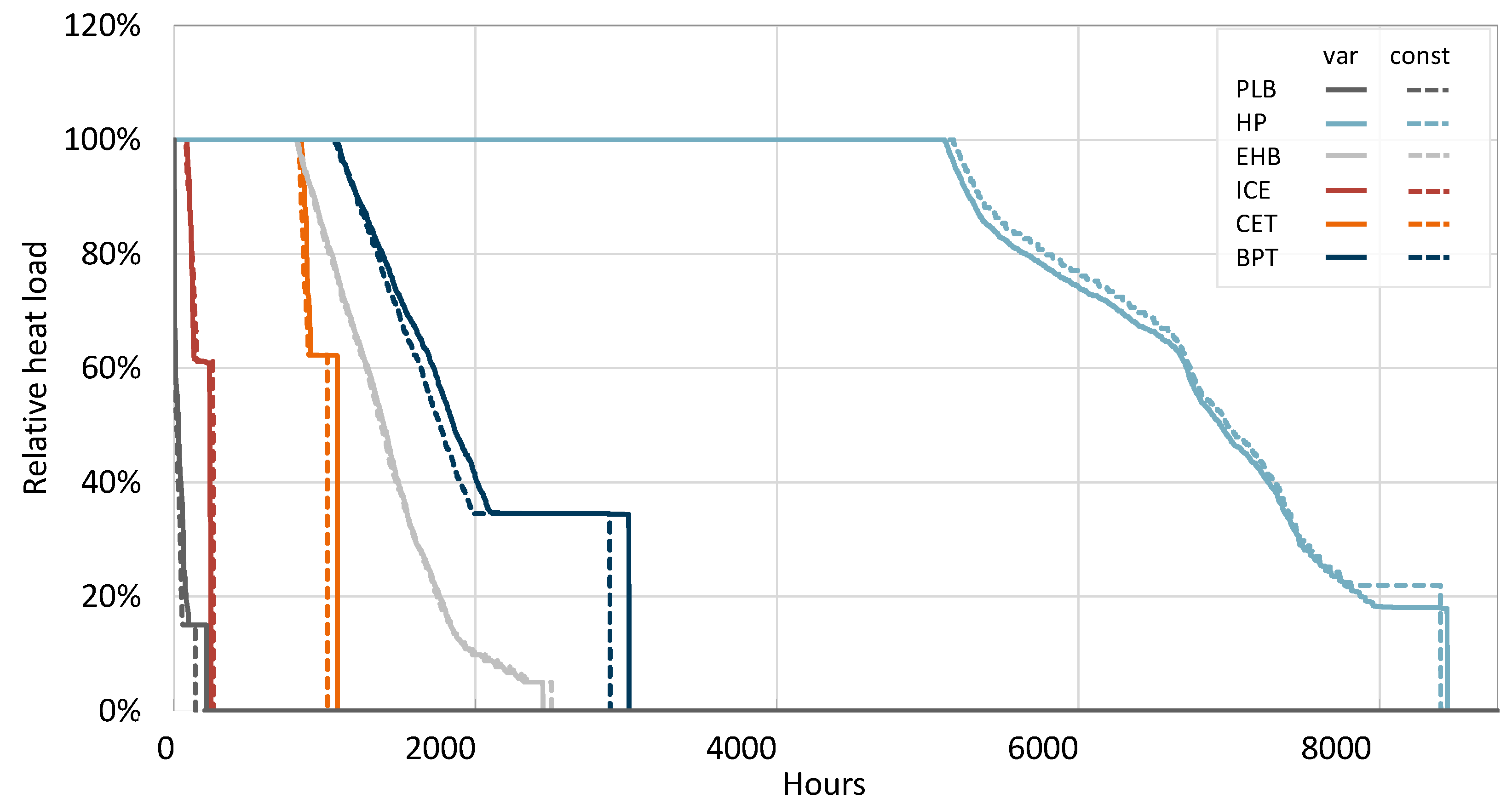
Examples of results for the technology dispatch are shown in Figure 5 as load duration curves for the variable and constant medium supply temperature setup, in the PTH scenario. These curves depict the load of the heating technologies relative to the temperature-dependent maximum producible heat in a specific time step. Comparing constant and varying supply temperature setups, the load characteristics appear similar with a slightly steeper part load range for BPT and a higher minimum load for HP with constant supply temperatures. Additionally, the orders of the technology duration curves stay the same.

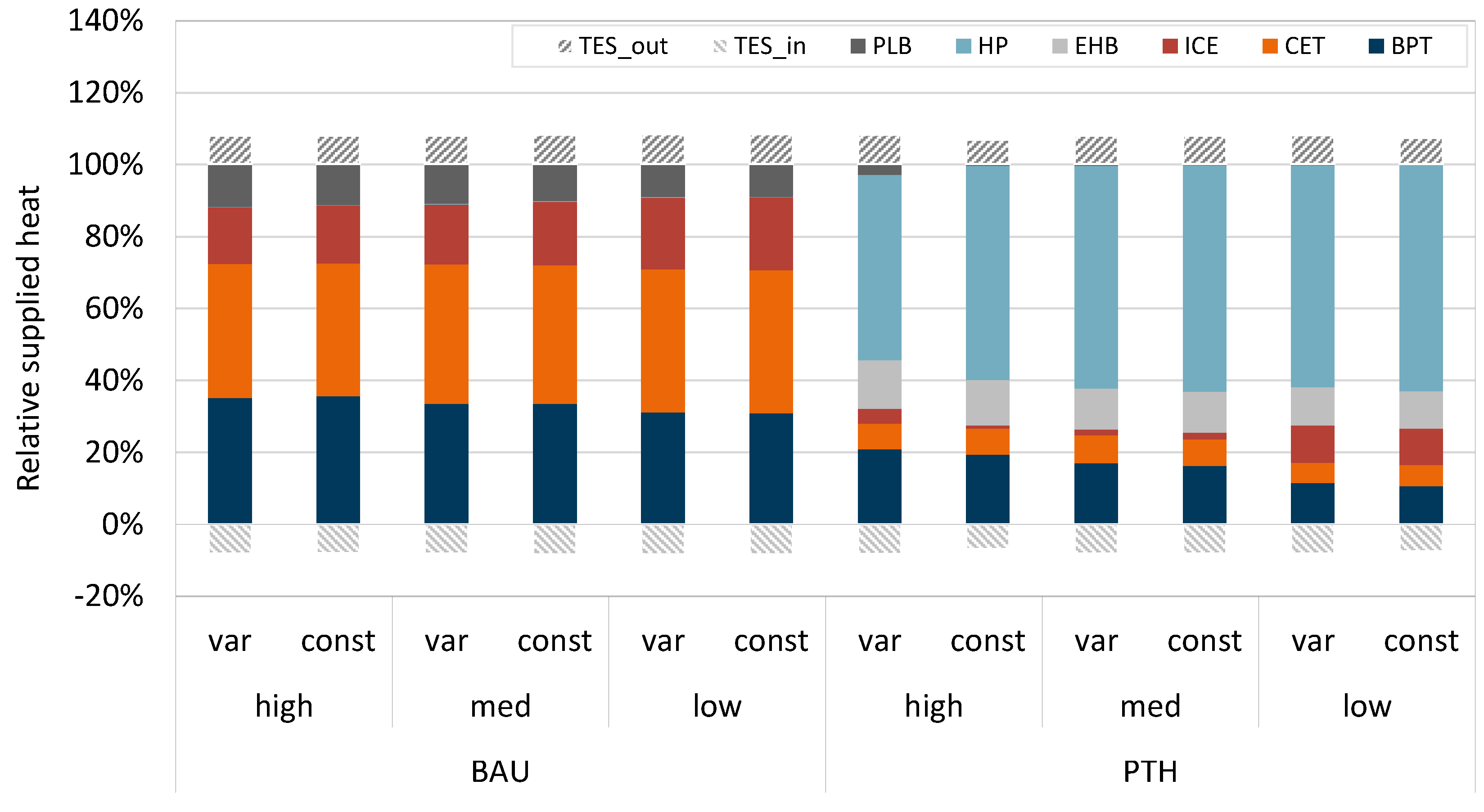
An overview of all optimized scenarios is given in Figure 6 as an annually summarized, technology-specific heat supply. As expected, the operational results for the BAU and PTH scenarios indicate significantly different heat supply structures. In the BAU scenario with variable high supply temperatures, CET and BPT, followed by ICE, dominate the heating system with a share of almost 90% of the heat supply. In the corresponding PTH-supportive scenario, the HP meets half of the heat demand. Furthermore, lower supply temperatures indicate generally increasing shares of ICE, CET, and HP, while operations of BPT, PLB, and EHB decrease. Overall, the comparisons of the operational results of the variable and constant supply temperature scenarios show marginal deviations at a maximum of 1% in the heat supply structure. An exception with deviations of up to 8% between the technology dispatch of variable and constant supply assumptions is shown under the PTH-supportive market conditions and high supply temperatures. In this situation, the maximum heat supply temperature of the HP restricts its operation in 891 h of the year when considering variable flow temperatures. In contrast, modeling the heating plant with the constant mean temperature of 91 ${}^{\circ }$C does not lead to any operational limitations.

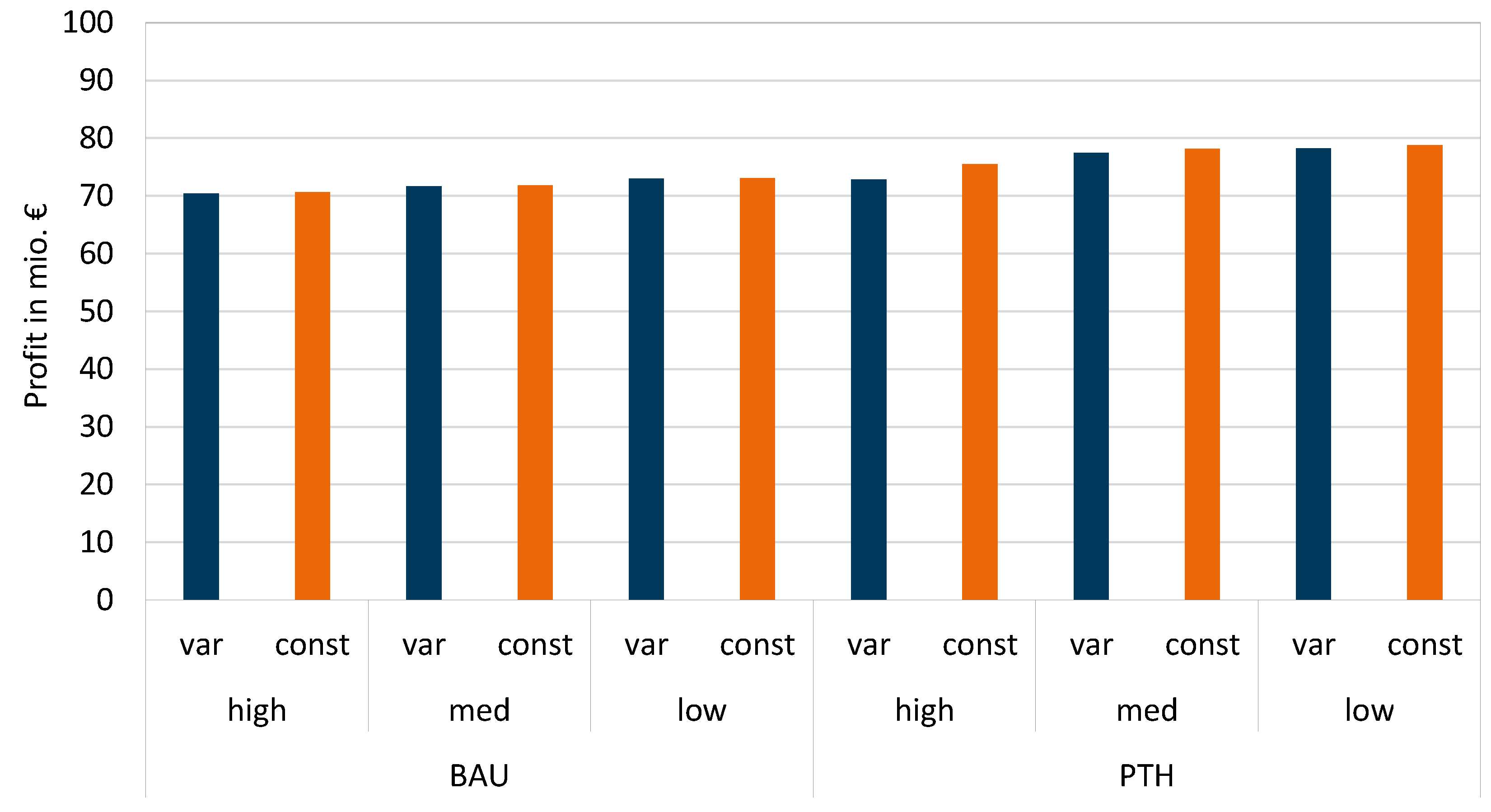
The chosen scenarios are further assessed in terms of profits, which include revenues, fuel costs, and other variable operating costs but no fixed operating costs, as shown in Figure 7. In general, the results range between 70 and 79 mio. EUR annually, whereby the PTH scenario entails higher profits in comparison to the BAU scenario. A comparison of the economic results for the different temperature levels indicates that slightly higher profits are reached with lower temperature levels. Furthermore, the profits based on the constant temperature integration are higher than their variable counterparts, due to slightly less part load operation at lower efficiencies. The deviations range between 0.2 and 0.9%, whereby the results for the PTH scenario lie in the upper end. Again, the temperature restriction of the HP leads to an exception at high supply temperatures under PTH-supportive conditions, with a deviation of 3.7%.

5. Discussion

The proposed model shows that varying supply temperatures in DH systems can be integrated in MILP models as flow-dependent operational parameters. These express the temperature dependence of the technical efficiencies and operational restrictions. Related formulations are implemented for CHP technologies and HP, but can be applied to EHB and PLB as well. In the present study, these are modeled with constant efficiencies due to minor variations. In contrast, further research is necessary to adequately represent TES in MILP models with varying temperatures, due to operational restrictions based on the resulting temperature stratification. On the basis of the case study, the functionality of the developed model was tested. Overall, the technology dispatch ensures the heat supply, while reacting to market price developments. In particular, the compliance of the technology operating points with their operational restrictions is proved. Thus, varying supply temperatures can be generally integrated in MILP models of future DH systems.

The application of the optimization model in the presented case study allows for analysis of the influence of the overall temperature level on the operational results in a DH system. Generally, the temperature level affects the technology dispatch and economic results. With lower supply temperatures, the heat supply shares of BPT, PLB, and EHB decrease while those of ICE, CET, and HP increase. With the rising share of those technologies and higher electrical efficiencies when distributing heat at lower supply temperatures, operational profits increase. But as the simulated BAU and PTH scenarios show, the extent of these variations strongly depends on the market environment. Under BAU conditions, lowering supply temperatures gradually shifts the dispatch between the single CHP technologies, and at the same time minor influences on PTH technologies can be observed. In contrast, in the PTH scenario the extent of dispatch variations is more significant which affects both CHP and PTH technologies. Thus, framework conditions have a much stronger impact on the technology dispatch in DH systems than temperature levels. A transformation towards a 4GDH system can only be achieved if those conditions are adjusted as lower flow temperatures are introduced, as already stated in Reference [1].

Additionally, the system transformation requires a DH assessment model that appropriately depicts technologies. Therefore, simplifications to reduce the computational complexity have to be analyzed in terms of result deviations. The influence of assuming practically varying supply temperatures with constant parameters is also quantified based on the case study. A comparison of the technology dispatch shows that the results of the constant temperature scenarios deviate from those of the scenarios based on variable supply temperatures. The extent of these deviations mostly amounts to a maximum of 1%. Nevertheless, when operational restrictions are met by either variable or constant supply temperatures, the result deviations become significant. Thereby, the extent depends on the frequency of occurrence of those circumstances, which is why these cases have to be examined separately. A similar behavior is verified for economic results. Based on these findings, a simplification of supply temperatures in DH system models can be applied in studies dealing with the transformation of heating systems. For a detailed analysis of the technology dispatch, the presented MILP model can be used with variable supply temperatures.

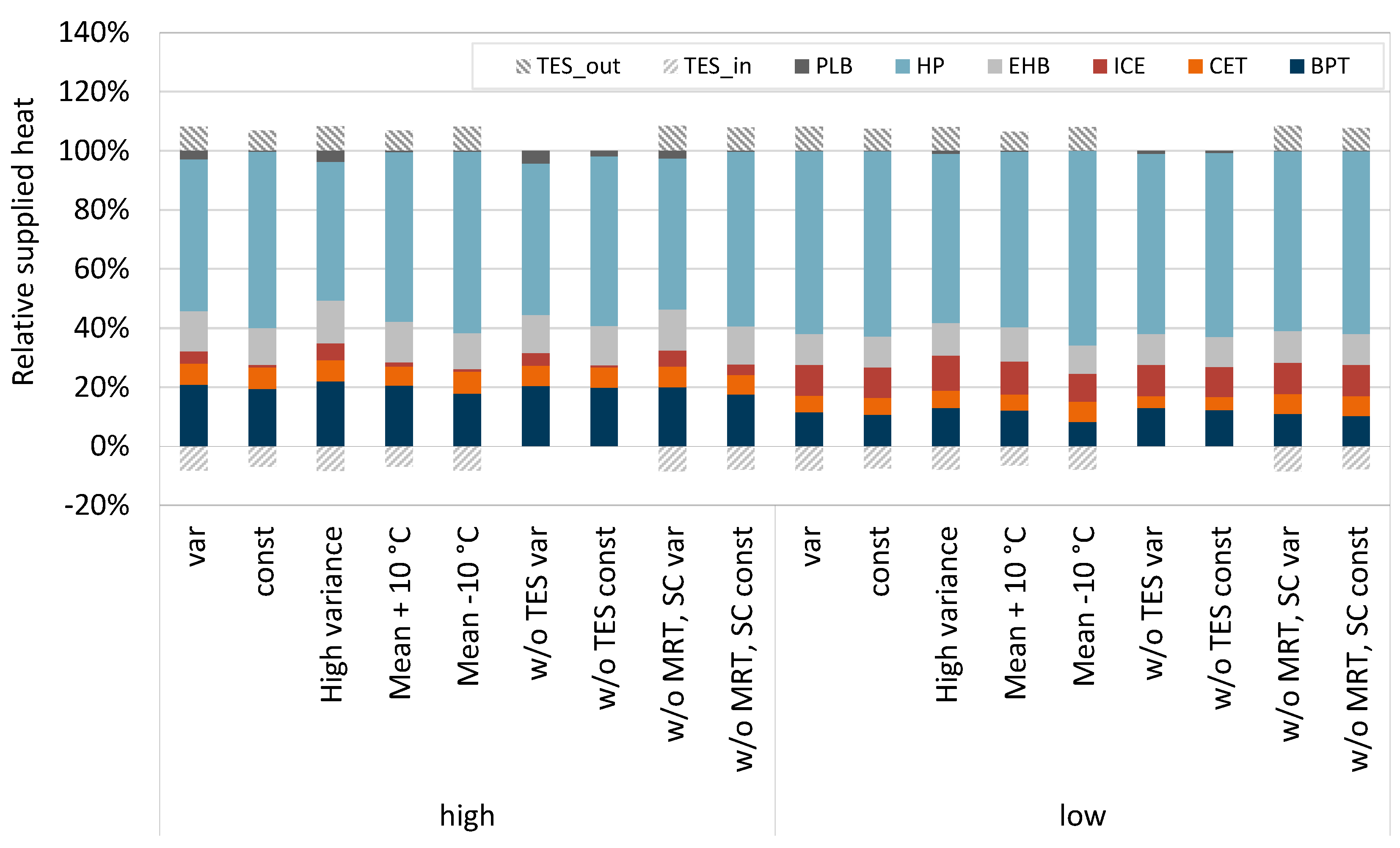
To support these findings a sensitivity analysis is conducted for the high and low temperature levels in the PTH scenario and is depicted in Figure 8. Increasing the variance of the variable temperature time series by a factor of 4 (high variance scenario), increases the differences of dispatch results compared to the constant assumption due to more frequently occurring operational restrictions. Furthermore, a less accurate estimation of the mean temperature as a constant (scenarios Mean $+{10}^{\circ }$C and Mean ${-}^{\circ }$C) does not lead to significant differences. Thus, the accuracy of assuming constant supply temperatures in DH models is dependent on the present temperature data and can be preserved in most applications. Further simulations comparing dispatch results without TES (scenarios w/o TES var and w/o TES const) show that technologies not modeled in great detail do not distort the presented research. The same is valid for a comparison study that does not take minimum runtimes and start costs into consideration (scenarios w/o MRT, SC var, w/o MRT, SC const).

6. Conclusions

The developed MILP model integrates varying supply temperatures in order to calculate the unit commitment of a DH plant consisting of established heating technologies. Temperature-dependent technology characteristics, efficiencies and operational restrictions, are pre-calculated by linear functions and expressed as flow-dependent operational parameters in the model. By analyzing the optimization results in a case study, the model is tested and can therefore serve as a proper investigation instrument for further research on DH systems.

The transformation path towards 4GDH systems is characterized by decreasing supply and return temperatures, which has an influence on the heat supply structure. Lower supply temperatures favor ICE, CET, and HP, while the other investigated technologies—BPT, PLB, and EHB—show declining operating hours. With this, potential operational profits increase. Nevertheless, the effect is comparably small as opposed to adaptions in the regulatory framework.

Furthermore, the case study shows that dispatch and economic results under constant supply temperature assumptions and their variable counterparts, deviate up to a maximum of 1%. Significant deviations of the optimization results are only found when either the variable or constant supply temperature setup affects technical restrictions. Based on these findings, simplifications in terms of assuming constant supply temperatures in DH models can be applied in studies of the transformation of heating systems, whereas a detailed analysis of the technology dispatch potentially requires the variable temperature integration in the proposed MILP model.

References

- Lund, H.; Werner, S.; Wiltshire, R.; Svendsen, S.; Thorsen, J.E.; Hvelplund, F.; Mathiesen, B.V. 4th Generation District Heating (4GDH). Energy 2014, 68, 1–11. [Google Scholar] [CrossRef]
- Bloess, A.; Schill, W.P.; Zerrahn, A. Power-to-heat for renewable energy integration: A review of technologies, modeling approaches, and flexibility potentials. Appl. Energy 2018, 212, 1611–1626. [Google Scholar] [CrossRef]
- Christidis, A.; Koch, C.; Pottel, L.; Tsatsaronis, G. The contribution of heat storage to the profitable operation of combined heat and power plants in liberalized electricity markets. Energy 2012, 41, 75–82. [Google Scholar] [CrossRef]
- Rieder, A.; Christidis, A.; Tsatsaronis, G. Multi criteria dynamic design optimization of a small scale distributed energy system. Energy 2014, 74, 230–239. [Google Scholar] [CrossRef]
- Dimoulkas, I.; Amelin, M. Constructing bidding curves for a CHP producer in day-ahead electricity markets. Energycon 2014, 487–494. [Google Scholar] [CrossRef] [Green Version]
- Wille-Haussmann, B.; Erge, T.; Wittwer, C. Decentralised optimisation of cogeneration in virtual power plants. Sol. Energy 2010, 84, 604–611. [Google Scholar] [CrossRef]
- Navarro, J.P.J.; Kavvadias, K.C.; Quoilin, S.; Zucker, A. The joint effect of centralised cogeneration plants and thermal storage on the efficiency and cost of the power system. Energy 2018, 149, 535–549. [Google Scholar] [CrossRef]
- Dimoulkas, I. District heating system operation in power systems with high share of wind power. J. Mod. Power Syst. Clean Energy 2017, 5, 850–862. [Google Scholar] [CrossRef] [Green Version]
- Ommen, T.; Markussen, W.B.; Elmegaard, B. Heat pumps in combined heat and power systems. Energy 2014, 76, 989–1000. [Google Scholar] [CrossRef]
- Effenberger, H. Dampferzeugung; VDI-Buch, Springer: Berlin/Heidelberg, Germany, 2000. [Google Scholar]
- Bach, B.; Werling, J.; Ommen, T.; Münster, M.; Morales, J.M.; Elmegaard, B. Integration of large-scale heat pumps in the district heating systems of Greater Copenhagen. Energy 2016, 107, 321–334. [Google Scholar] [CrossRef] [Green Version]
- Hilpert, S.; Kaldemeyer, C.; Krien, U.; Günther, S.; Wingenbach, C.; Plessmann, G. The Open Energy Modelling Framework (oemof)—A new approach to facilitate open science in energy system modelling. Energy Strategy Rev. 2018, 22, 16–25. [Google Scholar] [CrossRef]
- Wärtsilä. Dynamic District Heating: A Technical Guide for a Flexibal CHP Plant; Wärtsilä: Vaasa, Finland, 2015. [Google Scholar]
- Haga, N.; Kortela, V.; Ahnger, A. Smart Power Generation: District Heating Solutions; Wärtsilä: Vaasa, Finland, 2012. [Google Scholar]
- Jarre, M.; Noussan, M.; Poggio, A. Operational analysis of natural gas combined cycle CHP plants: Energy performance and pollutant emissions. Appl. Therm. Eng. 2016, 100, 304–314. [Google Scholar] [CrossRef]
- Steag Energy Services GmbH System Technologies. EBSILON Professional 13; Steag: Zwingenberg, Germany, 2017. [Google Scholar]
- Algie, C.; Wong, K.P. A test system for combined heat and power economic dispatch problems. In Proceedings of the 2004 IEEE International Conference on Electric Utility Deregulation, Restructuring and Power Technologies, Hong Kong, China, 5–8 April 2004; Volume 1, pp. 96–101. [Google Scholar]
- Christidis, A.; Mollenhauer, E.; Tsatsaronis, G. Einsatz Thermischer Speicher zur Flexibilisierung von Heizkraftwerken. In Proceedings of the 47 Kraftwerkstechnisches Kolloquium, Dresden, Germany, 13–14 October 2015. [Google Scholar]
- Mollenhauer, E.; Christidis, A.; Tsatsaronis, G. Evaluation of an energy- and exergy-based generic modeling approach of combined heat and power plants. Int. J. Energy Environ. Eng. 2016, 7, 167–176. [Google Scholar] [CrossRef] [Green Version]
- Blarke, M.B. Towards an intermittency-friendly energy system: Comparing electric boilers and heat pumps in distributed cogeneration. Appl. Energy 2012, 91, 349–365. [Google Scholar] [CrossRef]
- Mancarella, P. Cogeneration systems with electric heat pumps: Energy-shifting properties and equivalent plant modelling. Energy Convers. Manag. 2009, 50, 1991–1999. [Google Scholar] [CrossRef]
- Fatouh, M.; Elgendy, E. Experimental investigation of a vapor compression heat pump used for cooling and heating applications. Energy 2011, 36, 2788–2795. [Google Scholar] [CrossRef]
- Steck, M.H.E. Entwicklung und Bewertung von Algorithmen zur Einsatzplanerstellung virtueller Kraftwerke. Ph.D. Thesis, TU München, München, Germany, 2013. [Google Scholar]
- Blarke, M.B.; Dotzauer, E. Intermittency-friendly and high-efficiency cogeneration: Operational optimisation of cogeneration with compression heat pump, flue gas heat recovery, and intermediate cold storage. Energy 2011, 36, 6867–6878. [Google Scholar] [CrossRef]
- Gomez-Villalva, E.; Ramos, A. Optimal energy management of an industrial consumer in liberalized markets. IEEE Trans. Power Syst. 2003, 18, 716–723. [Google Scholar] [CrossRef] [Green Version]
- Salgado, F.; Pedrero, P. Short-term operation planning on cogeneration systems: A survey. Electr. Power Syst. Res. 2008, 78, 835–848. [Google Scholar] [CrossRef]
- Bischi, A.; Taccari, L.; Martelli, E.; Amaldi, E.; Manzolini, G.; Silva, P.; Campanari, S.; Macchi, E. A detailed MILP optimization model for combined cooling, heat and power system operation planning. Energy 2014, 74, 12–26. [Google Scholar] [CrossRef]
- Wang, H.; Yin, W.; Abdollahi, E.; Lahdelma, R.; Jiao, W. Modelling and optimization of CHP based district heating system with renewable energy production and energy storage. Appl. Energy 2015, 159, 401–421. [Google Scholar] [CrossRef]
- Boettger, D.; Goetz, M.; Theofilidi, M.; Bruckner, T. Control power provision with power-to-heat plants in systems with high shares of renewable energy sources—An illustrative analysis for Germany based on the use of electric boilers in district heating grids. Energy 2015, 82, 157–167. [Google Scholar] [CrossRef]
- Schuetz, T.; Streblow, R.; Mueller, D. A comparison of thermal energy storage models for building energy system optimization. Energy Build. 2015, 93, 23–31. [Google Scholar] [CrossRef]
- Kaldemeyer, C.; Boysen, C.; Tuschy, I. District Heating Modelling Data for the Publication “Integration of Feed Flow Temperatures in Unit Commitment Models of Future District Heating Systems”. Available online: https://doi.org/10.5281/zenodo.2553876 (accessed on 6 February 2019).
- Stadtwerke Flensburg GmbH. District Heating Network Data for the City of Flensburg from 2014–2016. Available online: https://doi.org/10.5281/zenodo.2553967 (accessed on 6 February 2019).
© 2019 by the authors. Licensee MDPI, Basel, Switzerland. This article is an open access article distributed under the terms and conditions of the Creative Commons Attribution (CC BY) license (http://creativecommons.org/licenses/by/4.0/).