Article

Building Variable Productivity Ratios for Improving Large Scale Spatially Explicit Pruning Biomass Assessments

by
Daniel García-Galindo
1,*,
Arkadiusz Dyjakon
2,* and
Fernando Cay Villa-Ceballos
3
1
Research Centre for Energy Resources and Consumption (CIRCE), 50018 Zaragoza, Spain
2
Institute of Agricultural Engineering, Wroclaw University of Environmental and Life Sciences, 51-630 Wroclaw, Poland
3
Department of Mechanical Engineering, University of Zaragoza, 50018 Zaragoza, Spain
*
Authors to whom correspondence should be addressed.
Energies 2019, 12(5), 957; https://doi.org/10.3390/en12050957
Submission received: 8 February 2019 / Revised: 28 February 2019 / Accepted: 7 March 2019 / Published: 12 March 2019
(This article belongs to the Section L: Energy Sources)

Abstract

:
Biomass assessments of agro–residues performed at large geographical scales generally base calculations on single constant pruning productivity ratios (RSRs). Reliability of biomass assessments shall be improved if RSRs respond to prevailing regional crop growing conditions. The present paper describes the methodology applied to create geographically varying pruning RSR ratios–tons of dry matter per hectare—for five crop groups: vineyard, olive, fruit species, citrus and dry fruits. A newly created database containing 230 records–from seven EU28 countries—is submitted to statistical analysis. Results reveal that agro-climatic conditions are able to explain a not negligible share of the pruning productivity as dependent variable. Subsequent regression analysis provides two equations—for vineyard and citrus—achieving a reasonable good fitting (R2 0.18 and 0.42 respectively) between RSR and the agroclimatic variables. Analysis of olive, fruit species and dry fruits scatter and whisker plots were useful for zoning and inducing ramp functions. A Geographical Information System (GIS) was utilised to apply the functions to the agroclimatic raster coverages in order to obtain RSR raster grids. Zonal statistic procedures applied by European regional units (NUTs0, NUTs2, NUTs3) provide a specific crop RSR ratio per administrative unit as a principal output of the present work.

1. Introduction

Biomass assessments in large (global, regional or national) scales have been object of multiple research efforts for providing estimations and scenarios of biomass availability. The objective of large-scale biomass estimations is usually to provide an overview of biomass availability as first step for preparing biomass action plans, or regional strategies for promoting new biomass supplies. In such large scale works, agricultural residues assessments have usually started from agricultural statistics and yearbooks (global, regional, national and subnational data). These sources of information provide relevant figures on the agricultural sector like distribution of crop species, cultivated land, crop yields and productions, historical series, production value or market indicators, among others. Among the variety of figures presented in agricultural databases and yearbooks, the assessment of agricultural residues have usually based on two records: either (a) the cropped area and, or (b) the crop production. Starting from these two variables, the methods applied usually calculate the biomass potentials through ratios of residue productivity, respectively: (a) productivity per unit of land area, usually called Residue to Surface Ratio (RSR) expressed as kg·ha−1 or t·ha−1; (b) productivity of the residue per unit of agricultural product, so called Residue to Product Ratio (RPR) as ton of residue per ton of crop product [1,2,3].
The result of this calculation is the usually called theoretical potential or total biomass potential. The theoretical potential is the basis for further more specific estimations like the available biomass—which discounts from the theoretical potentials those resources already in use—, the technical collectable potential—for which it is precise to know the amount of residues that can be collected—, the economic potential— includes a model of costs to identify the amounts that can be utilised at lower costs—, or the sustainable potentials—those economic resources compatible with sustainability use—. For such estimations it is precise to count on with detailed data and experience on the biomass harvesting at field and economics [4] and on the conditions that could limit the utilisation of the resource—like environmental or agronomic regulations—.
In respect the assessment of theoretical potentials—object of the present research—the reliability and accuracy of biomass assessments depend on the quality and accuracy of the underlying data utilized. García-Galindo et al. [3] exemplified the dispersion and variability of the data on which biomass assessments usually base: land, crop yield and biomass productivity ratios. They observed tremendous variability in all variables, meaning that confidence interval—as statistical estimate—was not able to provide any additional information on the reliability and deviations of the assessments. In this sense, it was recommended a series of practices for complementing and discussing the results of biomass assessments, among them: detecting tendencies in the evolution of yearly data, obtaining appropriate ratios adequate for each geographical unit, or accompany the results of the biomass potentials with other complementary information (e.g., expected minimum and maximum values).
Reducing the uncertainty of biomass assessments via the appropriate incorporation of cropped areas and crop productions is already in practice via multiple paths: utilization of yearly series, preparation of land use scenarios, or modelling future land utilization or crop production. There exist multiple research works which base their biomass estimations on complex models which procure the land use scenarios and land or crop production projections. In reference to those who already applied the methods to assess the potentials of agricultural residues for Europe it is worth mentioning two recent works developed in the framework of the European Research and Innovation funding 2014–2020 (known as 7th Framework Programme): Biomass Futures (http://www.biomassfutures.eu/) [5] and S2Biom project (www.s2biom.eu) [6]. The works carried out in both projects intended to provide biomass assessments and a strategic analysis to support policy makers in preparing their policies on biomass supply. Their strength in the assessment of agricultural residues—also pruning—biomass relies on the projections of land dedicated to growing permanent crops in 2020 and 2030. The projections are obtained by integrated outputs of models like Common Agricultural Policy Regionalised Impact (CAPRI) and GLOBIOM (http://www.globiom.org/) as explained by Elbersen and co-workers [7]. These models predict direct and indirect land demand based on economic models that simulate the agricultural and timber (commodity) production in response to markets and trade relations between countries. The models find the equilibrium between demand and supply and facilitate as output the land that is foreseen to be in use. Then the land is presented by subnational units (NUTs2 and NUTs3) thus providing a more precise assessment in geographical terms.
The mentioned studies assess the biomass potentials by multiplying in each territorial unit (NUTs2 and NUTs3) the hectares—output of the land use scenarios by 2020 and 2030—of land dedicated to each group of crops by the corresponding biomass productivity ratio (t·ha−1). The efforts and accuracy placed to obtain land projections are in contrast with the limited certainty of the productivity ratios. Biomass Futures [5] obtained the biomass for pruning biomass using a constant productivity ratio by crop species in whole Europe. S2Biom [6] obtained it using fixed RSR ratios (t·ha−1) by crop groups (fruits, nuts, citrus, olive and vineyards) and by country. A constant ratio was assigned to each of the countries object of assessment. The assignation based on the average ranges of RSR values published by EuroPruning project for nine European countries [8]. S2Biom assigned an average country value according to similarities in climate and geographic region (e.g., Belgium was assigned with Netherlands RSR values). In contrast to the limited reach in certainty of the S2Biom approach in respect the productivity ratios for pruning residues, herbaceous residues productivity was estimated per NUTs2 unit by using the ramp functions developed by Scarlat and co-workers at European scale [9].
Panoutsou and co-workers [10] provide a series of conclusions as a wrap-up of their experience in a book chapter published in 2017 after end of S2Biom project. Specifically about pruning residues, they conclude that further improvements are necessary, specifically:
  • generation of a harmonized inventory of permanent crops (olive, wine, fruit) throughout Europe integrating already existing databases and remote sensing information,
  • further field research to quantify residue ratios at local level and integrating into harmonised assessments through modelling.
In respect improvements in pruning productivity, ENEA—the Italian National Agency for New Technologies—has developed specific regional productivity ratios for the Italian Regions (NUTs2) and Provinces (NUTs3) [11] (pg. 3). The novelty lies in the fact that each geographical unit was assigned with the average value of a series of RSR values obtained by direct measurement in fields. This approach involves dedicated field sampling—weighing of residues—in different zones of the area of study. When facing large scale areas of studies, gathering the different combinations of factors that can influence the residues productivity implies a dedicated sampling campaign comprising: multiple sites sampling and multiple plot repetitions per site. The method is to be applied by crop, or by crop groups, meaning an enormous demand of efforts and resources in case of large-scale biomass assessments. This method would require unaffordable efforts when facing the assessment in large areas. This is the principal reason why currently large-scale assessment of agro-residues potentials usually constrain to the use of single RPR or RSR ratios constant in the whole area of study.
Herbaceous residues—by far those with largest potential in Europe—have been object of recent improvements. It is worth mentioning the referential works developed by Scarlat and co-workers [9,12], and by Fischer and co-workers [13,14,15] (the latter in the framework of IIASA-FAO Global Agro Ecological Zoning–GAEZ approach). Both work teams have developed ramp functions to assess the productivity of annual crops herbaceous residues: the former (Scarlat and co-workers) to wheat, rye, oats, barley, maize, rice, sunflower and rapeseed; and the latter (Fischer and co-workers) to the previous crops and additionally millet, sorghum, potatoes, sugar beet and soybean. These ramp functions express the ratio of residue productivity per unit of product – RPR as a function of the crop productivity. The ramp function is utilised to calculate the specific RPR value in each geographical unit (grid cell, municipality, province or region), which, multiplied by the value of crop production (e.g., tons of wheat grain) provides the estimate of the biomass potential in per geographical unit.
Differently to annual crop residues, none of the mentioned research groups developed ramp functions for assessing pruning biomass residues. They used constant ratios, as argued by Scarlat [12], because of the current lack of information about pruning biomass productivity ratios. The scarcity of dedicated and precise biomass assessments for pruning residues produced in the management of olive groves, vineyards and fruit plantations is evidenced by the fact that in 2011 the pruning biomass potentials across the Europe have not been considered. Only two of the European National Renewable Action Plans (NREAP for Spain and France) included this potential. In contrast, straw was quantified in 14 NREAPs, and agro residues (as a whole) and energy crop potentials reported in more than 20 NREAPs. A second evidence is the usually limited reach of pruning biomass assessments in current works carried out at large scale, as exemplified with the mentioned approaches of Scarlat and co-workers [9,12], Fischer and co-worker [13,14,15], Biomass Futures project [5] or S2Biom project [6].
Improving the certainty of pruning biomass assessments—as is pointed out by Panoutsou and co-workers [10]—is a necessary step as regard of the meaningfulness of pruning residues as a still scarcely mobilised biomass resource, with relevant potential for Europe. Biomass from pruning operations carried out to olive, fruit and vinestocks (usually referred as permanent crops) can play a role as an alternative and not negligible source of biomass in Europe. Permanent crops occupy 6.4% of the agricultural area in Europe, being the third group of crops in relevance: annual crops circa 60% of the agricultural land and permanent grasslands circa 32% (according to Eurostat data for EU28 [16]). Even though the area of permanent crops is a small share of the EU agricultural land, the residues produced with pruning have a significant potential since a relevant part of the residues produced remains unexploited and thus available for energy uses [17]. The sustainable use of pruning biomass for Europe could reach about 10 million tonnes of oil equivalent (Mtoe)·yr−1 by 2030, whereas biomass still not utilized from annual crops and from released permanent grasslands could add 50 Mtoe·yr−1 and 3.9 Mtoe·yr−1 respectively [5]. Furthermore, this source of biomass can have a prominent role in areas (rural principally) where olive, grape and fruit are prevailing crops. In such zones a change of the paradigm could lead to a relevant rise in the supply of biomass, thus contributing to sustain the new bioeconomy activities in Europe.
The present paper describes transparently a new methodology scoped to obtain pruning biomass productivity ratios—either RSR or RPR—tailored to local regional prevailing crop growing conditions. This contribution is aimed to enrich and improve the materials for assessing pruning biomass potentials in large scale studies. The methodology has been developed in the framework of the European project EuroPruning (FP7-KBBE-312078 contract) between 2013 and 2016. The methodology developed is inspired by the Scarlat and co-workers [9,12] equations prepared for annual crops, which residue productivity RPR was expressed as function of the crop yield. Here the methodology is applied to pruning biomass productivity in vineyards, olive groves and fruit plantations, and is expanded to explore other multiple factors that affect the productivity of pruning residues.
The work performed is vast, and wide in data sources and methods. The description of singular details of the database construction, the statistical analysis (including 39 crop and agroclimatic variables and multiple sample segregation attempts) and the implementation of results is beyond of the rationale of a research article. Therefore the present work gathers the principal elements of the methodology and results to facilitate its replication. Particular details are referred when necessary to already published materials like project reports [17,18] or partial communications [8,19]. This incorporates supplementary information (unpublished maps and tables) obtained for Europe. This work may facilitate replication, thus allowing improvements in the databases and productivity ratios of the biomass assessments on agricultural pruning at large scale.

2. Materials and Methods

2.1. Focusing the Methodology

2.1.1. State of Art of Large Scale Biomass Assessments Using Non-Constant Ratios

The present work is inspired by the method applied by Scarlat and co-workers [9,12] to obtain a set of adjusted curves correlating the productivity of agricultural herbaceous residues (RPR expressed as kg of residue per kg of grain) with the crop yields (kg of grain per hectare). The authors identified diverse causes leading to large variability of residues productivity along the European territory: crop type, production systems, yields, climate, soil conditions (among other factors) and the varied agronomical practices (e.g., use of irrigation). The mentioned works reduced the uncertainty of their assessments at European [9] and national (Romania) [12] scale by developing RPRs which value was dependent on the crop yield. Their methodology resulted satisfactory in order to achieve an improvement in the assessment of the agricultural residues produced by annual crops, and thus findings and results have been utilised by other works assessing biomass potentials in: Europe [6,20,21], or even out of the European context (e.g., in Asia [20] or Argentina [22]).
For the development of their methodology Scarlat and co-workers [9,12] posed as starting hypothesis that the amount of agricultural residues is directly related to crop production. Assuming such hypothesis, their work concentrated in finding correlations between the productivity of the residue and the crop yield. They selected as dependent variable the RPR instead of the RSR. Their approach started with a literature research from where multiple RPR and corresponding yields were gathered. Subsequently they performed an analysis of correlations between the RPRs and crop yields.
The fact that a single independent variable (the crop yield) was utilised is briefly discussed by authors in both research works [9,12]. They argue the residue production depends on a number of factors that include: the types of crops and crop variety, the general crop management (density, tillage system, crop rotation, crop mix, degree of intensification), local agro-ecological conditions (climate and precipitation pattern, soil properties, etc.), the weather during the current campaign (frosts, droughts) and the farming techniques applied along it (irrigation, fertilisation, pest management, etc.). The use of a single independent variable can be justified as both crop yield and crop reside are affected intrinsically by same factors. Notwithstanding the hypothesis assumed by Scarlat and co-workers (yield as principal variable to explain the variations in RPR values), they acknowledge that some factors could affect differently crop yield and RPR.
Scarlat and co-workers suggest that crop residue productivity is even more variable than crop yields. Additionally to the factors also affecting yield, crop residues productivity are affected by harvesting techniques, the cutting height and the inherent inaccuracies when performing the field measurements. They performed a research work to find evidences of the correlation between RPRs and yield and concluded that the correlation is not simple and straightforward: whereas under certain conditions several works reporting the crop yield keeps a direct and positive relation with the residue production, other works stated an inverse relation [9] (pg. 1891).
Scarlat and co-workers applied the methodology and succeeded in developing the aimed functions correlating RPRs with crop yields for multiple herbaceous crops. The data on RPRs and yields were gathered from diverse literature sources was segregated by crop, and then plotted (dispersion diagram RPR vs. yield). The best fit curves between yield and RPRs were produced for each type of crop: wheat, barley, maize, oats and rye, rice, rapeseed and sunflower. All these crops were analysed separately in the work performed at European scale [2]. In contrast for Romania [12] the analysis was not performed for rice, and some crop types were analysed together: wheat and barley, and oats and rye. The sample sizes per crop (or crop group) ranged 30–40 in the work performed at European scale [9], and 20–60 in the study for Romania [12]. The correlations found between the RPR and crop yield achieved a limited fitting with R2 0.17–0.28. This was evaluated as an evidence of correlation. However, R2 values ranging 0.17–0.28 indicate that the models explain approximately only from 17 to 28% of the changeability in the quantity of biomass obtained. In other words, that yield itself was only able to explain partially the changes in RPR values.

2.1.2. Changeability of Pruning Productivity as Dependent Variable

Prior the preparation of the methods for the present work, a literature research was carried out to identify other works which could have developed equations or models dedicated to provide values of the pruning residues productivity ratios—either RPR or RSR—varying spatially. No report or research was found but a deterministic approach developed by ENEA (the Italian National Agency for New Technologies, Energy and Sustainable Economic Development) and AIGR (Italian Agricultural Engineering Association) where different RPRs were proposed by NUTs3 level [23] on the base of field data measured in different zones. Beyond this work no single assessment—carried out at large scale—has been found before the initiative of the EuroPruning project and the release of the present paper.
Notwithstanding the absence of works at large scale, two research teams had produced alometric equations correlating the pruning productivity with diverse dendrometric and agronomic variables. Both research teams developed their work locally: areas of homogeneous climate, both in Eastern Mediterranean coast of Spain. The methodology included systematic sampling (measurement of residue productivity and dendrometry, and observation of other variables), followed by an exhaustive statistical analysis of correlation, and the development of regression models. Velázquez-Martí and co-workers developed four referential works building regression curves for pruning productivity per hectare (RSR). The species sampled were: vineyards [24], olive groves [25], citrus [26] and almond plantations [27]. Velazquez-Martí and co-workers considered as independent variables dendrometry (tree or branch diameter, tree height, crown height and crown diameter) and plantation agronomy (crop yield, age, density and irrigation). They also analysed the influence in the RSR of crop variety, architecture of tree, aim of pruning or pruning intensity (type of pruning work). The second work team (Fernandez-Puratich and co-workers) developed a dendrometric model to estimate volume of wood in fruit trees [28], including a specific model for assessing volume of wood in branches.
Both works achieved good correlations and fitting of the regression models for RSR. Velazquez-Martí and co-workers achieved R2 always above 0.50 and typically 0.6–0.7 using as predictive variables dendrometric parameters, management factors and crop yields, and segmenting when necessary by influencing factors like market orientation of the production (grape or wine), subspecies or pruning type. Fernández-Puratich and co-workers developed regression models based on dendrometric variables. They achieved R2 above 0.9 for the volumetric models of tree branches (not the pruning, but the branch as a part of tree), based on data obtained in very homogeneous plots in terms of climate, density, variety, soil conditions, irrigation, weather and altitude over sea level. The good fitting indicates the models were able to explain a relevant part of the changeability of the branches growth and thus, of the pruning productivity.
The mentioned works state the possibility to predict RSR as dependent variable as function of dendrometric data, yields and diverse plantation characteristics. The present work considers both types of influencing variables. Beyond them, several factors have been identified as influencing the pruning residue productivity. A list of factors—arranged in different group classes—is proposed next. The list and groups derive from the discussion of results carried out by Velázquez-Martí and Fernández-Puratich in their respective publications, from the conversations with sectorial specialists—performed during EuroPruning project surveying work—, and from the descriptions provided in diverse horticultural treatises. The factors identified are arranged into six groups, as next:
  • Crop: inherent characteristics of plant species. Not influenced by crop management. Factors include: species, variety, plant age. Variety is a crucial factor as there exist varieties with different vigour, and different evolution of the annual vegetative growth.
  • Agro-ecological conditions: not inherent to the plant, but to the local conditions: climate type, precipitation, temperature regime, weather during last crop cycle (affecting the stage of vegetative growth, and crop yield), soil.
  • Agronomics: the practices performed by the farmers to adapt the crop variety to the local prevailing agro-ecological conditions. Among them they have been identified: crop conduction or form (vase, trellis, palm, etc.), plantation density, degree of irrigation, input of fertilisers and pesticides, pruning frequency (formation, annual, biennial, renovation), pruning system (manual, mechanised, combined) and pruning intensity in previous campaigns—since residue generation depends on the needs for crop shaping: the more a tree becomes untreated, the larger amount pruning wood expected—. All these aspects on agronomics are very varying from plantation to plantation, as they depend on the abilities, means and preferences of the farmers or plantation managers.
  • Market: evolution of markets changes the demand on product—fruit, grape or olive—quality, variety or size, among others. It may influence a more intense fructification pruning (clearing at start of reproductive stage to obtain pieces of larger size, e.g.,). As well plantations adhered to a PDO (Protected Designation of Origin) may be requested on specific agronomics, whereas other plantations may follow very different practices.
  • Human factors: referring to other facts usually difficult to trace, and that may lead to unusual execution of agronomics. They may affect pruning productivity (e.g., in case of lack of personnel, a lighter pruning shall be carried out), or the fruit productivity (e.g., if size is preferred to volume of production, plantation yield is lower).
  • Crop yield: it is the seasonal result of all previous factors: crop and variety, local conditions, agronomy applied by farmers, special singular weather events and human influence. Yield can refer to the average plantation yield, or to the fruit yield harvested the season before the pruning is executed.
The mentioned factors may have an effect on the pruning productivity. A complete description and discussion on the factors can be found in a previous EuroPruning report [17] and communication [19], to which we refer for a further insight. Special remark deserve the human factors. Experts and farmers consulted, as well as horticultural publications, state that the human factor is quite influencing in the result of pruning operations. Pruning operations are carried out usually by farmers or workers with shears plant by plant. Every person has a different way to perceive the need of pruning, and that leads to different intensity and thus to different amount of residues. This factor cannot be registered or easily traced. Additionally there are other human factors affecting the amounts produced yearly. For example, in crops requiring some periodic renovation of the principal conducting branches, some farmers wait for five or ten years to perform it; in contrast others perform operations of renovation or restructuring of the canopy yearly, by cutting off unproductive or damaged branches, performing special cuts for re-conducting branches, or eliminating those too high or of large dimension. Another case is the buffering of results when a farmer is monitored by researchers, since the person may perform more accurate or more intense pruning than usual in the sampled trees. In cases when continued rains fall during the pruning campaign, the pruning operations may undergo delays, and then a less intense pruning may be applied, to be compensated with a more intense pruning in the next campaign

2.2. Methodology Scheme of the Present Paper

The methodology applied to pruning residues in the present paper follows Scarlat and co-workers approach [9,12]. The correlation between multiple factors presented in Section 2.1.2 and the productivity of pruning residues is explored here with aim of obtaining predictive equations applicable to large-scale assessments. Differently from Scarlat and co-workers, who selected yield as the single and unique independent variable for their correlation study, here all factors are initially considered in the correlation study. Two dependent variables are the productivity ratios: either RSR, or RPR—the latter requiring a record of crop yield in each surveyed site.
The methodology is presented as a sequence in the next list, and in same order in the following sections:
  • Definition of the variables to count on for the influencing factors, and potential sources of information.
  • Data collection: preparation of the data gathering (according to the reach and means available inside the EuroPruning project action), data collection (from published articles or singular experiences, complemented with information directly surveyed from authors), and consolidation of the database.
  • Statistical analysis of the database:
    analysis of correlation between the independent variables selected and the dependent variables (RPR and RSR) in order to select those variables with a proved relation with the dependent variable;
    analysis of regression (linear) including the compliance of the hypothesis (confidence, independence, heteroscedasticity, normality in the distribution of residues) to ensure statistical consistency of the mathematical expressions found. This is a standard statistic approach to perform regression analysis, and is equivalent to the methods followed by Velázquez-Martí and Fernandez-Puratich teams. Regression analysis goes beyond the straightforward curve fitting method presented by Scarlat and co-workers;
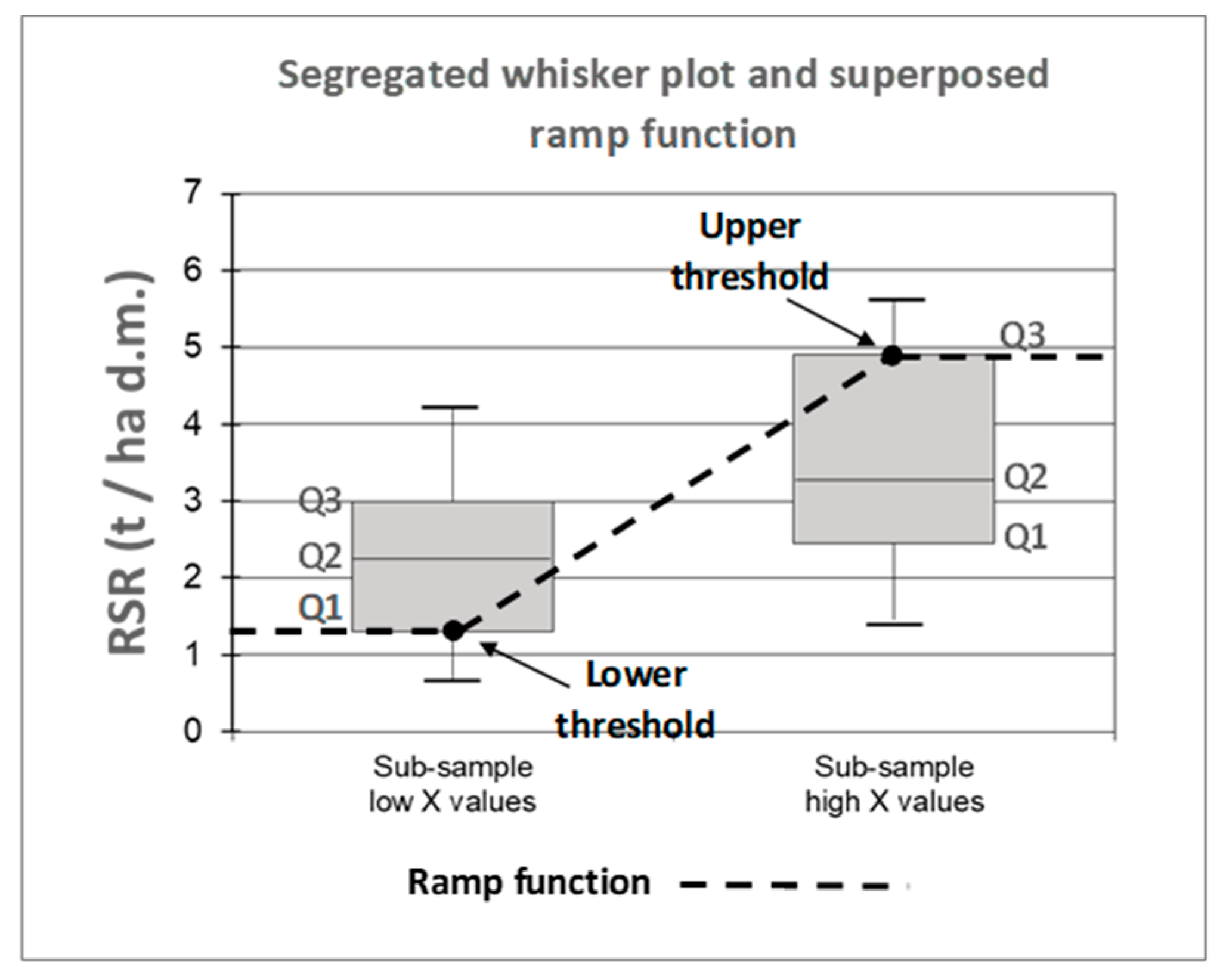
    visual analysis of the scatter and whisker plots in the sought of evidences of a growing or decaying tendency of the dependent variable—RSR or RPR—in respect to the growth of the independent variable.
  • Preparation of ramp functions (based on the mathematical expressions found in the regression analysis) by following the methods of Fischer and co-workers [13,14,15]);
  • Application of the ramp functions with the values of the independent variables to determine the average pruning productivity ratios per administrative unit—NUTs0, NUTs2 and NUTs3—in Europe.

2.2.1. Definition of Variables

Section 2.1.2 has presented a comprehensive list of factors influencing the pruning productivity. It is however, not possible to cover all of them. Firstly because it is needed to obtain values of RSR or RPR as function of variables typically contained into existing agricultural databases: agricultural yearbooks, national census, geographical coverages. These sources of information offer a limited amount of variables to base the assessment: crop types, areas, yields, plantation age, varieties, densities, climate type, rainfall, among others. However it is rare to count on with agricultural inventories describing any dendrometric data—differently to forestry inventories, which usually include it—like stem diameter. Even though dendrometric variables showed good ability to predict the pruning yield according to the conclusions of Velázquez-Martí [24,25,26,27] and Fernández-Puratich [28], these variables should not be considered for building regressions in large-scale assessments. A second reason constraining the implementation of some variables is the difficulty to convert them into quantities or dichotomous information. For example the agronomic factor describing the intensity of the pruning operation applied—e.g., “more intense pruning than usual”—cannot be implemented in form of variable. This information however may be useful for segregating the database, or for detecting outliers.
Table 1 summarises the parameters and variables utilised in the present work. As observed, they consist mainly in data easily available from publications—or by contacting authors of publications— or by consulting local experts in an area. They cover six groups of variables presented in Section 2.1.2. Each parameter (type of factor) is described by its name, the type of variable (nominal, dichotomous, ordinal, continuous) and acronym of the variables (one or more) implemented. That is, each factor can be traced by several parameters, and each parameter characterised by means of diverse variables. Table 1 marks the crop, plantation and agronomical factors that are represented intrinsically by each variable. The form how these variables include the mentioned factors is presented, and classified as: directly (the variable is itself the value of the factor); intrinsically (not explicitly, but the variable value is in reality influenced by one or several factors); through a calculation (when a variable is the result of a calculation based in the values of several factors) or equation; or through a model (in case the variable has been obtained by running complex models counting multiple factors). As observed there is a significant amount of agro-climatic and agro-ecologic parameters—16 in total—and variables—30 in total—. Climatic parameters refer to climate classifications or indicators. Agro-climatic variable include crop indicators (like suitability or agro-climatic potential or gross attainable yields) derived from a computing of the plant phenology adaptation to the prevailing climatic conditions, performed by means of computing models like CGIAR-CSI [29,30], ECOCROP [31] and FAO-IIASA [32]. Agro-ecological variables go beyond agro-climatic indicators and include effects of soil or pests, and are gathered in this paper from FAO-IIASA [32]. These set of climatic, agro-climatic and agro-ecologic variables are obtained from open accessible databases. Table 1 shows how agro-climatic and agro-ecologic variables take into account multiple factors like crop type, weather, or some basic agronomics. In case of yield—actual yield, not the modelled yields—it is observed that it incorporates naturally all factors, as yield is, in the end, the result of the plantation growth and production.
In total each registry of the database contains a total of 39 variables, representing 25 different parameters (as presented in Table 1). The description of each variable can be consulted in detail in the EuroPruning deliverable D3.1 [17].
Performing consistent statistical analysis requires well-populated database. In order to create a sample of sufficient size the methodology to record registries of pruning productivity included two approaches:
  • Surveying local experts: a survey was created to contact local experts who may have recorded pruning productivity in previous campaigns.
  • Literature: research or technical publications containing data of pruning productivity (derived from field sampling) or pruning mechanical collection tests (where t·h−1 and t·ha−1 are monitored). As result of an initial analysis, it was stated that publications usually did not contain all information needed. A direct contact with authors based on the survey was performed as a necessary complement.
Each register includes relevant data for the analysis like: specie and variety, planting pattern, crop form, plantation and renovation age, type of irrigation (if any), pruning season, frequency and type of pruning (manual, mechanical), pruning productivity, moisture content (measured or estimated), and current management of pruning (burning in the field, shredding and burying, household firewood, etc.). Other complementary information was included like coordinates (latitude, longitude), origin of the data, persons who contributed, and description of the area or region represented, among others. As well, some subjective fields designed to detect or explain outliers in the statistical analysis: cases when pruning productivity was higher than other years, the field is more productive or more vigorous than others, or there existed any specificity that made the plantation differ from other average plantations.
The data on climatic, agro-climatic, agro-ecological and yield variables provided by global models was obtained from the grids publicly available (see data sources in Table 1). The values of these indicators were read from the geographical coverages in the coordinates of each register, and then the values linked to the corresponding register. The operations have been carried using a geographical information system (QGIS v2.14-Essen, Open Source Geospatial Foundation, Beaverton, OR, USA). Further details can be consulted in the EuroPruning report on pruning potentials) [17].

2.2.2. Statistical Analysis

The analysis is performed with IBM SPSS Statistics 19 (IBM Corp., Armonk, NY, USA). Standard methods available in this statistical package are followed to carry out the different steps of the statistical analysis.
Correlation analysis
A correlation analysis detects which of the selected variables present evidence of correlation with the dependent variables (RSR or RPR). Detecting a correlation may indicate that the occurrence of the dependent variable (pruning productivity) could be explained in some degree by the independent variable analysed. Its strength can be checked through different methods and coefficients. The use of Spearman coefficient (ρ) has been selected. Similarly to Pearson or Kendall correlation methods, Spearman is a bivariate analysis that measures the strength of association between two variables. It also provides the direction of the relationship. This method is specially of interest as is well suited to detect monotonic relations for either continuous or ordinal variables. This is an advantage in respect to Pearson correlation method, which is appropriate for continuous variables which are expected to show normality and present linear correlations. Additionally the information provided by the Spearman coefficient includes the review of simple scatterplot to detect visually evidences of direction, linearity or normality.
Spearman correlation method analyse the matrix with the data of dependent and independent variables, and provides as result:
  • The strength of the relation or the value of the coefficient ρ, which varies in the range 0–1, with values nearest to ρ = 1 denoting a strong correlation
  • The reliability of the relation or the p-value: only significance correlations with a confidence level of 0.05 are accepted in the present work—p-value < 0.05, meaning that there is only 5% of probability that the relation is due to coincidence and not representative of the population tendency—.
  • Possible multi-collinearities or relations between pairs of independent variables. Variables that are collinear have a relationship among them. When performing the regression analysis, independent variables should be independent between each other.
Regression analysis
The regression analysis aims to provide mathematical expressions where the dependent variable is calculated as function of a series of independent variables. Regression analysis was not applied to variables with low coefficient of correlation because of two principal reasons: firstly the fact that the good fitting of the regression curve depends on the strength of the correlation between the independent and dependent variable. Thus, variables showing low correlations are expected to not produce well-fitted models. Secondly, because in absence of an evidence of correlation, a regression analysis may provide curves, even though there has not been proved the existence of any real connection between the independent and dependent variable.
A linear regression analysis was applied to those variables which showed a good correlation with the dependent variable (pruning productivity, denoted here as RSR). Building regression curves followed standardised statistical methods. IBM SPSS Statistics 19 was utilised for performing the regression analysis, as well as to check the consistency of the regression. The tests carried out to check such consistency are: homoscedasticity (to check the homogeneity of the variance), normality (following Kolmogorov-Smirnov method) and independence (through Durbin-Watson statistic).
Linear regression models were selected as the best alternative to build mathematical expressions. A reason behind is a lack of any evidence that the functional correlation between pruning productivity and any of the independent variables chosen is logarithmic or potential. Differently, alometric regression of forestry species have shown in multiple works such potential or logarithmic relations, as for example between the aboveground biomass and the diameter at breast height (DBH) of the tree stem. As a matter of fact, Velázquez-Martí [24,25,26,27] and Fernández-Puratich [28] built non-linear functions based on dendrometric variables predicting the pruning or the branches productivity. These models achieved very good fitting R2 values always above 0.5 and up to 0.9. However, for the present study, where the independent variables are agronomic, climatic, agro-climatic and yield parameters, the method of linear ramp functions proposed by Fischer and co-workers in their works [13,14,15] has been followed. Ramp functions (as depicted in Figure 1) include a linear central zone along the width of the X-values of the sample distribution. Beyond these limits the value of the ramp is made constant. Ramp functions are a good-practice to prevent the use of regression curves out of the range of values on which the regression analysis based. An extrapolation out of the limits requires a well informed decision. Since ramp functions show a central part of linear growth (or descent) the scatter plot accompanied the regression analysis in order prevent from applying linear functions in cases where clear non-linear tendencies could be observed.
Whiskers plot and zoning
The statistical approach of correlation and regression models require good fitting of the data to provide results with acceptable values of R2. There are cases when correlation analysis may indicate an existing correlation between the dependent variable (RSR or RPR) and one or several independent variables. However the subsequent regression model may fail in the consistency, or may show a very poor fitting (low values of R2). Once a correlation has been evidenced, the scatter plot and whisker plot analysis may be useful to observe a tendency of the RSR or RPR values to be low or high, in different zones of the plots. Velázquez-Martí and co-workers [24,25,26,27] utilised this method to show the increase of the pruning productivity when a data series was segmented. The scatter plot is divided in zones according to the visual interpretation. A whisker plot is prepared for each one of the zones detected. The visual analysis of whisker plots may be useful to observe typical behaviour of the dependent variable, and useful for proposing ramp functions for those variables showing moderate or good correlations, but not able to produce a consistent regression model.

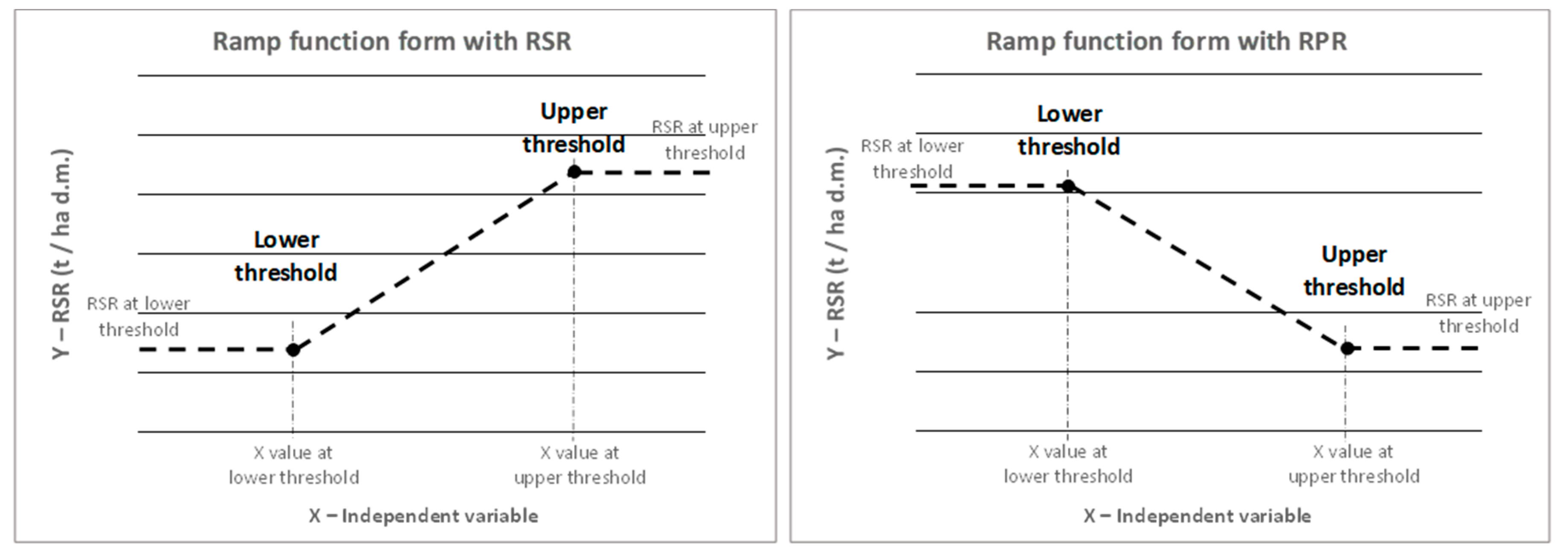
2.2.3. Building Ramp Functions for RSR or RPR

Ramp functions have been utilized by Fischer and co-workers in several works [13,14,15] to model RPR as function of crop yield. The method is here explained. The first step is determining if a positive or negative correlation is foreseen between the dependent variable—RSR or RPR—and each independent variable. This is marked in Table 1 with symbols plus and minus in the corresponding column. As Fischer and co-workers explain, the relation of RPR with yield is expected to be inverse, since cultivars of higher yielding varieties aim at a higher shares of the primary productivity to be stored in the harvested parts. As a consequence, RPR is generally lower as compared to lower yielding traditional cultivars. In contrast, RSR is expected to be positive with yields—or in the case of the present work with the values of computed agro-climatic and agro-ecological variables—since the better the crop adapts to a climate, the larger vegetative growth (accumulation of material in structural parts of the plant) and the larger crop yield. In the present work, these tendencies are the starting point to build ramp functions. A ramp function for RSR and RPR is presented in Figure 1.
Next step is determining the expected range of values for the dependent variable. These upper and lower values of the range are denoted as upper and lower function thresholds. Subsequently it is necessary to assign to the upper and lower threshold a value of the independent variable. The ramp function is created by assuming a linear growth between the point of lower and upper threshold. Beyond the upper and lower thresholds the value of the dependent variable—RSR or RPR—remains constant. It is therefore crucial the right selection of the values at the upper and lower threshold to prepare the ramp functions. This selection is performed by the decision making of the research team —as Fischer and co-workers did [13,14,15]—by interpreting the underlying objective data.
In the case when a regression model has been obtained for a crop, the equation of the model is converted into a ramp function. The lower and upper limits are set according to the limits of the sample on which the regression model was built. Inside this interval of values, the linear function utilized is the expression obtained by the regression model. Beyond of these limits, the use of the linear regression is inadvisable, since it may incur in unexpected deviations. Thus the solution, as proposed by Fischer and co-workers [13,14,15] is to keep the value of the ratio—RSR or RPR—constant (see Figure 1).
In case the regression analysis failed, but the statistical analysis evidenced a correlation—thus meaning that the dependent variable can be explained partially with the values of the independent variable—the visual interpretation of segmented whisker plots is the alternative to build ramp functions. The visual interpretation aims to find out if the dependent variable show smaller or higher values grouped in zones of the X-axis. If such growing/decreasing tendency is detected, and the tendency is coherent with the sign of the correlation analysis and the foreseen tendency—as expressed in Table 1—then a ramp function can be implemented. The sample is segregated in two parts: dots at the side of low X values (low values of the independent variable) and dots in the side of high X values. These two sub-samples are presented in form of whisker plots. The values of the Quartile 1 (Q1) and Quartile 3 (Q3) are utilised to set the value of the dependent variable at the points of lower and upper thresholds (Figure 2). In case the independent and dependent variable have a positive correlation (case of the pair crop yield—RSR) then the Q1 of the sub-sample on the left side of the plot is assigned to the Y coordinate of the lower threshold, and Q3 of the sub-sample at the right-side assigned to the Y coordinate of the upper threshold. The assignation of Q1 and Q3 is the reverse in case the dependent and independent variables show an inverse correlation. The selection of the X coordinate at the lower and upper threshold is obtained from the visual analysis of the scatter plots. The method is visually depicted in Figure 2, where ramp function is superposed to the segmented whisker plot.

2.2.4. Preparation of Spatially Explicit Ratios

QGIS v2.14—Essen has been utilised to apply the ramp functions at European scale. The independent variables are expressed in form of spatially explicit data (continuous raster grid coverage). The values of the ratio RSR or RPR are calculated with the use of raster calculation tools. The equation is introduced in the raster calculation module and the raster calculator re-calculates the value of each pixel in the map to obtain the value of RSR or RPR. Ratios can be obtained both for rainfed and irrigated conditions when the variable is available in such format.
The raster coverages of RSR or RPR are the base to obtain averaged values of RSR or RPR by NUTs2 and NUTs3 geographical units. To avoid the buffering of the zero values—grid cells where the models show no suitability of the crop to grow—in the calculation of the average value per geographic unit, the grids with value equal to zero must be screened out. This operation is performed in the present work by assigning value “null” (no value) to these cells. The result is a new coverage which cells contain either “null” value, or a “non-zero” value of RSR or RPR. The average value of the ratio RSR representative in a specific NUTs unit is obtained by applying zonal statistics functionality available in QGIS v2.14 spatial analysis tools.

3. Results and Discussion

3.1. Database Implemented

Data has been obtained for seven countries: Spain and Italy with the largest number of records, France, Germany, Poland, Greece, Portugal and Croatia. An initial database of 261 records has been created: 158 records from literature sources and contact with authors, and 103 records from surveys carried out to local experts or cooperatives in seven countries. The consistency and completeness of each record has been reviewed, and contacts performed if necessary with authors of publications or local experts. A total of 31 records were discarded, as being considered either incomplete or not reliable. Data of the crop yields could not be recorded for multiple of the records coming from literature. Authors visited fields to perform the weighting of pruning biomass, though not always asked or registered the average crop yield or the crop yield in the season before the pruning operation was carried out. Therefore building RPR values has not been possible, and for the present approach only the RSR can be object of analysis as dependent variable. The final database contains a total of 230 valid records, which are described in Table 2 and depicted in Figure 3.
Table 2 reveals a considerable variability of the RSR values. As observed, the standard deviation is high in all cases. When observing minimum and maximum values, the difference is as well quite wide, ranging from very low productions ranging 0.1–0.3 ton of dry matter per hectare and year to up to 6.0 t d.m. per hectare. The ratio between maximum and minimum is from one to two orders or magnitude—ratio max/min from 9 in citrus species to 137 for pome fruits—. When examining the coefficient of variation (percentage of standard deviation with respect of the mean value, expressed as percentage) the values range from 46 in vineyard to 129 for nuts.
The high variability can be explained as regard of the diverse ages and cropping systems that have been included in the database. However, the minimum and maximum values are extreme points, probably inherently including some facts not well traced by the data gathering method: age, seasonal weather effect—which may have affected the vegetative growth of the tree structure—or influence of human factor—like too light or too intense pruning—. These facts illustrate the richness of the data collected, and the difficulty to explain the pruning productivity with a sole factor.

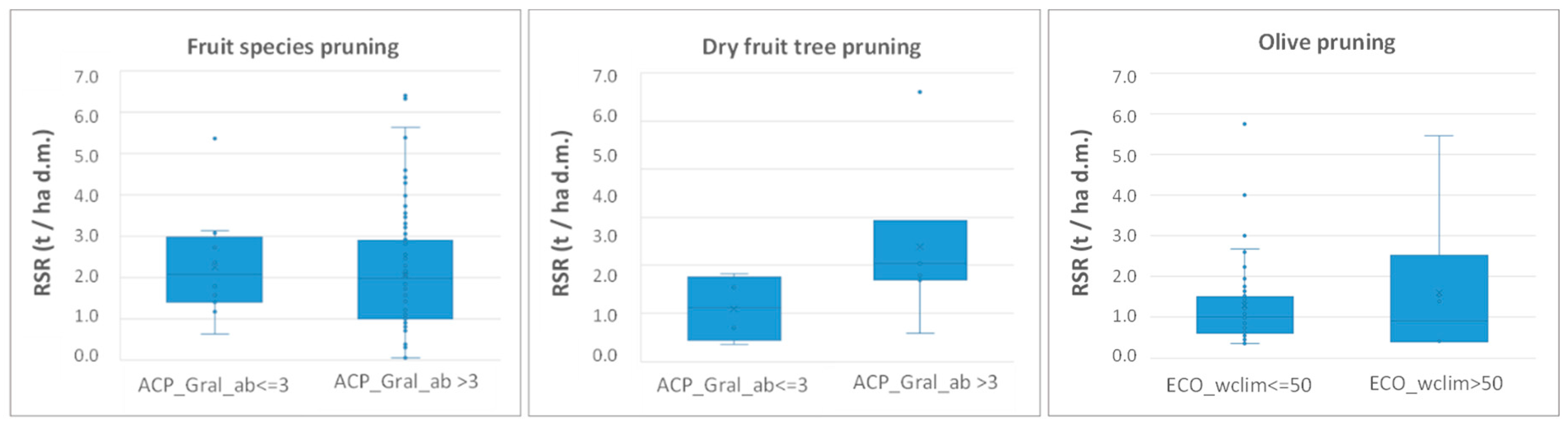
3.2. Residue to Surface Ratios Correlation Analysis

The analysis of correlation revealed that the degree of association measured by Spearman correlation is in general weak or very weak for most of the independent variables analysed. Table 3 contains the results of a set of seven variables showing an acceptable correlation, covering six groups of factors defined initially by the methodology (Table 1). Variables like crop form, irrigation or climatic region have been utilized for segregating the sample in the sought of finding better correlations when the correlation analysis is applied to more homogeneous sub-samples. Other variables not included in Table 3 revealed to not be relevant, or to be collinear (especially in case of climatic, agro-climatic and agro-ecologic variables).
As observed in Table 3 the Spearman correlation (ρ) is always lower than 0.6, except in a singular case. Agronomic-like variables resulted in general in low values for the Spearman correlation. Even more, some of the variables are not easily explained: for example the inverse relation between RSR and intensification: it would be expected that under a more intensified management—involving also a full coverage of the nutrient and water requirements of the plant—the vegetative growth were also larger. Climatic, agro-climatic and agro-ecological show a slightly better correlation with RSR.
The correlation found between the variables and RSR could be considered weak depending the scope and science branch. In case of dendrometry works, like those performed by Velázquez-Martí [24,25,26,27] and Fernández-Puratich [28], it is usual to expect values of ρ above 0.8. The mentioned collected the data through systematic and controlled sampling, and thus are subject of lower uncertainty. Additionally the sample was obtained in areas homogeneous in terms of climate and plantation management, which reduces the dispersion of values and the changeability.
In the case of the present work, the changeability is much higher due to the heterogeneous conditions under which the crops are being grown along Europe. Furthermore, the data has been compiled from different sources of information, and not by direct sampling. This involves higher uncertainty and thus, an additional impact in the variability of RSR—as caused by the method of data collection—. The human factor is a crucial issue not easy to be covered when the pruning operations are under study. As explained before in Section 2.1.2, pruning is performed manually, and is quite affected by human factors, like the person who performs the work, if the pruning is being carried out carefully or hastily, the preferred crop training system, etc. The methodology followed did not include direct sampling, and thus the human factor was not possible to be traced.
The total of 39 variables implemented—to characterise a total of 25 parameters of 6 groups of influencing factors— denote that it cannot be expected that a single variable could explain the changeability of the RSR alone. Thus, the correlations were initially not expected to be strong or very strong. Given the multiple factors affecting pruning productivity, a variable with ρ = 0.3—and thus R2 = 0.09—would explain 9% of the RSR changeability, which is not at all a negligible fraction. In case a variable reaches ρ = 0.6—and thus R2 = 0.36—it would be able to explain 36% of the RSR changeability, which is meaningful.
An additional fact limiting the chances to obtain high values of ρ in the correlation analysis derives from the human factor which pervades the present study. On the one hand human factor is quite inherently present in the results of the pruning operations as exposed in the section discussing methodology. It implies larger changeability and uncertainty. On the other hand the indirect method utilised—based on surveys and consults to literature authors—involves furthermore new uncertainty. The results of the correlation study cannot be expected to achieve the levels of correlation of scientific dendrometric studies including direct sampling. These works shall find ρ < 0.5 to be a weak correlation. In contrast, in social sciences, where both the object of analysis and the method involves inherently high uncertainty associated to the human factor, consider correlations of ρ > 0.3 to be moderate, and ρ > 0.6 to be strong [35]. This classification has been followed to refer the strength of the correlations.
According to the principal results of the correlation analysis (see Table 3) the climatic, agro-climatic and agro-ecologic variables show better correlations, with a value of moderate correlation (ρ > 0.3) for all crop groups. Among them, at least one variable per crop group also complies with the requirement of significance (p-value < 0.05). At the light of these results, an early conclusion of the work performed is that climatic, agro-climatic and agro-ecologic variables are able to explain a not negligible part of the changeability of the RSR values.
An unexpected result is the inability of yield to capture, at least partly, the changeability of RSR. Previous works referred like Scarlatt [9,12] and Velázquez-Martí [24,25,26,27] found yield as a relevant variable explaining RSR values, at least partly. In the present work yields have been object of careful examination, as it was expected to be a relevant variable to be taken into account. However the real values of the average crop yield or crop yield of the last season before the pruning were not fully recorded. Therefore the yield variables were obtained from FAO-IIASA [32] datasets, by assigning to each record the value obtained when reading the value of the grid in the corresponding coordinates. The yields are only crop-specific for olive (Ylds_OL_ab, Yld_gaps_OL), whereas the rest of yield values correspond to an average yield of multiple crops, kind of an indicator of the agronomical potential of the site—Ylds_ab, Ylds_rel, Yld_gaps—, and thus becoming more a type of agro-ecological variable, instead the actual crop yield. This fact is agued to limit capacity of the modelled yields to capture the changeability of RSR.
Beyond of the analysis performed, segmentation was utilized as a tool to separate the sample in more homogeneous sub-samples—by subspecies, by density, by climate, by agro-climatic indicators—. The principal aim was to try finding better correlations of the variables with RSR in a more homogeneous and reduced sample. This approach resulted quite useful for Velázquez-Martí and co-workers [24,25,26,27]. The technique consists in dividing the sample into two or several sub-samples according to values considered logical for representing different realities—e.g., density > 600 in olive groves denote intensive or superintensive plantations—. The present work performed segmentation by splitting the sample in two parts; scatter plots were observed before deciding the partition of the sample. Efforts performed of such systematic approach are well described by García-Galindo and co-workers [17,19] and by Cay Villa-Ceballos [36]. The results did not provide better correlations, but in very singular cases, and thus, the approach was rejected.
As summary, the sample obtained from the surveys and publications may not ensure to reproduce the reality on the permanent crop pruning current state. It is argued that the size of the sample needs to be widened, at the light of the large amount of factors on which pruning is dependent. As well the uncertainty involved in the present work, which does not gather field data directly, but by surveying and collecting published data from third parties, shall have hindered the capacity to have more clear and concrete results in the correlation analysis.

3.3. Residue to Surface Ratios Regression Analysis

The object of the present work is to provide results useful for improving the biomass assessments at large scale the regression analysis. Climatic variables, differently to agronomic variables, are usually available at large scale in form of raster/grids datasets for the whole globe, or extensive territories. Therefore the use of such data is a convenient base for implementing improved large-scale assessments. Obtaining regression equations can be helpful to transform such raster datasets into new raster containing the foreseen values of pruning productivity.
The regression analysis was applied to all climatic variables shown in Table 3 achieving at least a moderate value of the correlation coefficient (ρ > 0.3). Agricultural variables were not utilised based on two arguments: firstly since they showed in general lower correlation; secondly, the regression curve obtained could not be utilised for assessing biomass potentials in Europe since there are no inventories indicating plantation densities, ages, or degree of intensification at European scale. The results have been communicated and discussed previously by García-Galindo and co-workers [19]. Among all variables, only two regression models (vineyard and citrus) were found consistent and reached a reasonable good fitting whilst accomplishing the requirements to consider reliable the results of the model. In case of vineyard, a linear regression model (see Equation (1)) was built using as independent variable the Ecocrop suitability index (ECO_wclim).
Ecocrop suitability index ECO_wclim is the output of a simple mechanistic model which matches the phonological basic temperature and rainfall needs of a plant with the climatic data. The score produced ranges from zero—crop not suitable to the temperature and rainfall ranges—to 100—totally suitable, reflecting no, or very low heat, coolness and water stress. The larger the value of ECO_wclim, the better the crop adapts and thus the expected larger vegetative growth and biomass accumulation. ECO_wclim has been run on the Ecocrop module built-in DIVA GIS v12 software [31]. The climatic database utilised correspond to the current world climate—WorldClim version 1.4 embedded into DIVA GIS software—. The software facilitates the selection of the crop—currently covers 2568 plant species—and the climatic database. The matching gives as result a grid with the value of the suitability index—here denoted Eco_wclim—covering the whole globe.
The regression model achieved a fitting of R2 = 0.181 (R = 0.426), meaning that the— linear model explains 18% of the RSR changeability. This is a good value if it is considered the high variability and the scale of the work done. Absolute standard errors are 0.590 t·ha−1 d.m., which represent the error for the prediction obtained by using the linear model. The regression model obtained fulfils partly the hypothesis for being consistent, but not all (confidence sig = 0.021; normal distribution of residues not normal). Therefore, the regression analysis results should be taken with caution:
RSRvineyard = 0.733 + 0.016 * ECO_Wclim
The regression model for citrus provides a moderate fitting with R2 = 0.412 (R = 0.62), meaning the model is able to capture circa 42% of the changeability. The independent variable utilised was the Ecocrop suitability index (which reflects the suitability of a crop to grow under the prevailing climatic conditions: precipitation and temperature regime). All of the hypothesis (confidence, independence, heteroscedasticity, normality in the distribution of residues) was accomplished:
RSRcitrus = −0.898 + 0.111 * ECO_Wclim
The results obtained are rather limited, as the current work has been able to find regression curves for two out of five crop groups under study. The regression analysis showed some models with acceptable values of R2 for fruit, dry fruit and olive tree species, though the conditions necessary for considering the models consistent failed. Notwithstanding these results, the statistical study has been able to identify several consistent correlations for all the crop groups and a set of principally agro-climatic and agro-ecological variables.
The results obtained in the present work come from standardised statistical correlation and regression analysis, similar to the approach followed by Velázquez-Martí and Fernandez-Puratich teams. These research teams achieved R2 typically above 0.6 using principally dendrometric variables in a sample of trees measured in zones of very homogeneous climatic characteristics. In contrast to these works, the present study has a different nature, and is more similar to the approach of Scarlat and co-workers [9,12]. These works inspired the present research and achieved similar results in terms R2 which ranged 0.17–0.28. Even though these works present a numerous list of fitting curves on the productivity of biomass residues (straw) from annual crops, the method applied was more straightforward, and the curves presented do not necessarily comply with the hypothesis necessary to be consider as consistent and reliable. Therefore the results of the present work shall be considered an advance in respect those already achieved for annual crops by Scarlat and co-workers.

3.4. Zoning through Dispersion and Whiskers Plots

Correlation between RSR values and climatic, agro-climatic or agro-ecologic values has been evidenced through the analysis of correlation. Even though the correlation analysis reflects these factors are able to explain a not negligible part of the RSR changeability of RSR, finding a linear correlation with single factors requires a good fitting of the data series. The regression analysis applied has not been able to provide linear models with good fitting for the crop groups: fruits, dry fruits and olive.
The alternative followed for fruit, and dry fruits and olive—crop groups for which the regression analysis failed—is to work out ramp functions from the interpretation of the scatter plots. For such purpose it is precise to perform a visual review of dispersion plots (RSR vs. independent variable) and whisker plots associated. The method consist in segregating the plot in two parts, and observe a difference in the mean values and the distribution of values between the two segregated parts. Being the RSR directly proportional to ACP_Gral_ab and ECO_Wclim, it is expected the left part of the plots to show lower average than the values on the right part. Results of the zoning analysis for the crop groups fruit, dry fruits and olive are presented in Figure 4.
The plots evidence that as expected, the value of RSR grows as the agroclimatic parameters do. This fact is less evident for the group of fruit tree species (Figure 4, left), even though as observed the scatter plot on the right (corresponding to points with values of ACP_Gral_ab in the high rank) show numerous dots with values of RSR much larger than 3 t·ha−1 d.m. Such behaviour is consistent with the interpretation of the climatic variables, since agroclimatic parameters quantify the crop potentiality to yield, measured in form of productivity (in case of ACP_Gral_ab) or as suitability index of the crop with respect the prevailing local conditions (ECO_Wclim). The larger productivity potential in a site, the larger capacity for developing a good vegetative growth by the crop, and thus, a larger amount of pruning production could be expected.

3.5. Ramp Functions

Ramp function preparation for the crop groups vineyard and citrus have based on the linear function obtained in the regression analysis (Equations (1) and (2), respectively), as observed in Table 4. The equations are considered valid for the range of values of the independent variable (Wclim) in the sample. The ramp function has been constrained to a less extended interval to avoid the deviations near the boundaries of the sample, and thus limited to the range of Wclim 20–60—which set respectively the position the lower and upper thresholds of the ramp function—.
Ramp functions for fruit, dry fruit and olive crop groups have been built on the base of the evidences of the whisker plots, since the regression analysis did not yield any consistent curve. The value of RSR for lower and upper thresholds has been assigned according to the values of the RSR distribution—first and third quartiles—for each of the segregated samples. The coordinates X-Y of the Lower- and Upper-threshold have been utilised to fix the equation of the ramp—being the independent variable ‘X’ the Agro-climatic variable and the dependent variable ‘Y’ the RSR value—. The results are presented in Table 4.

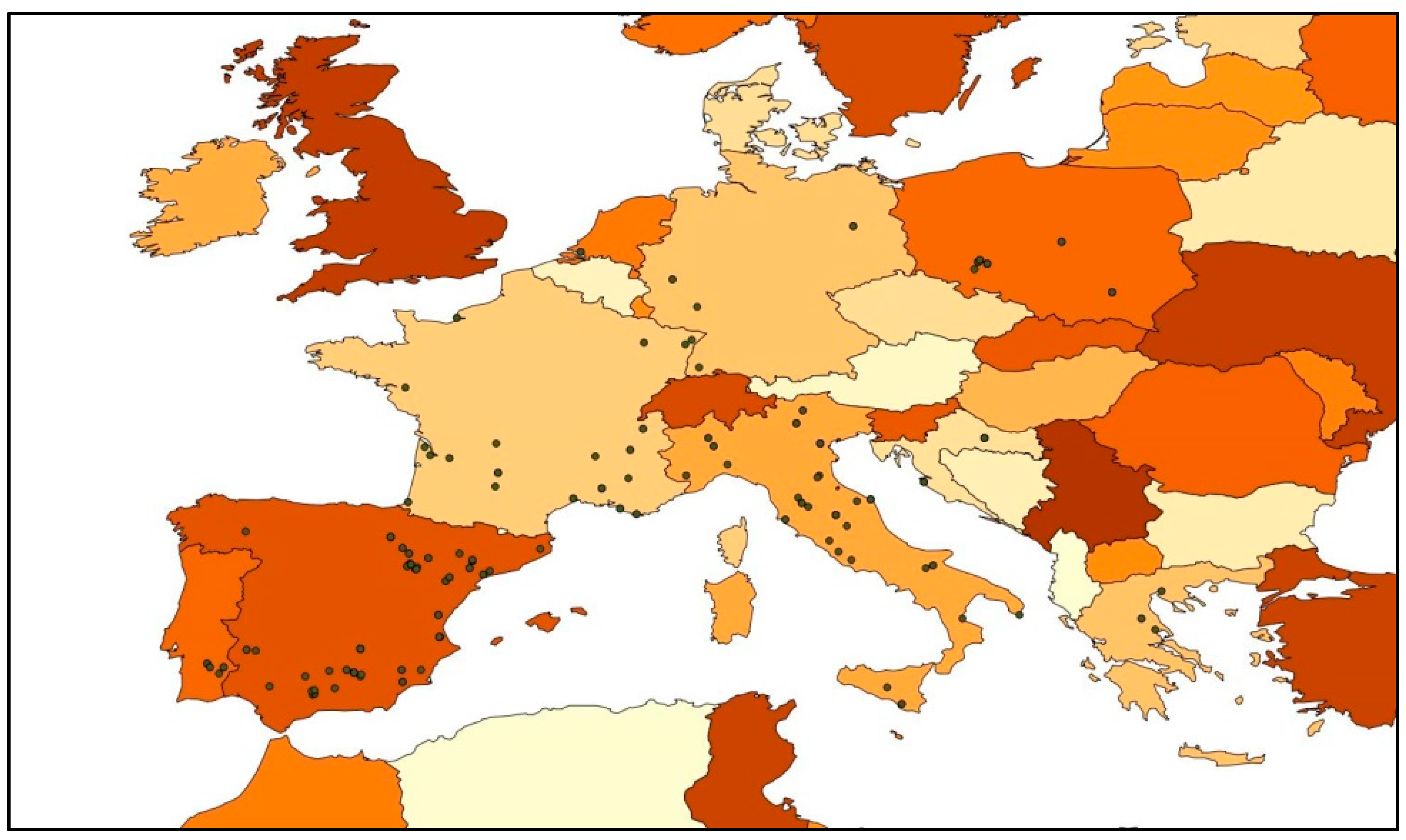
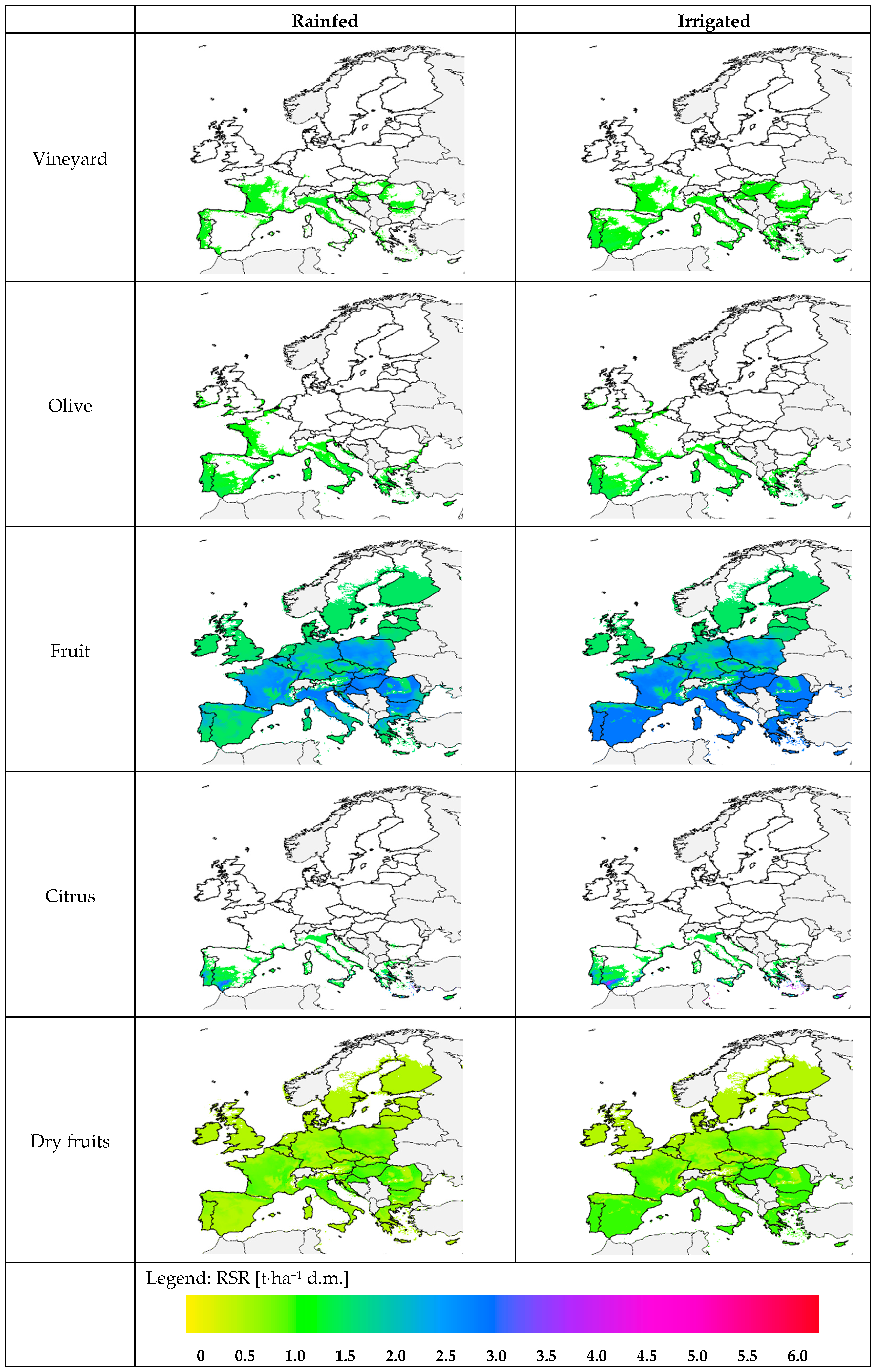
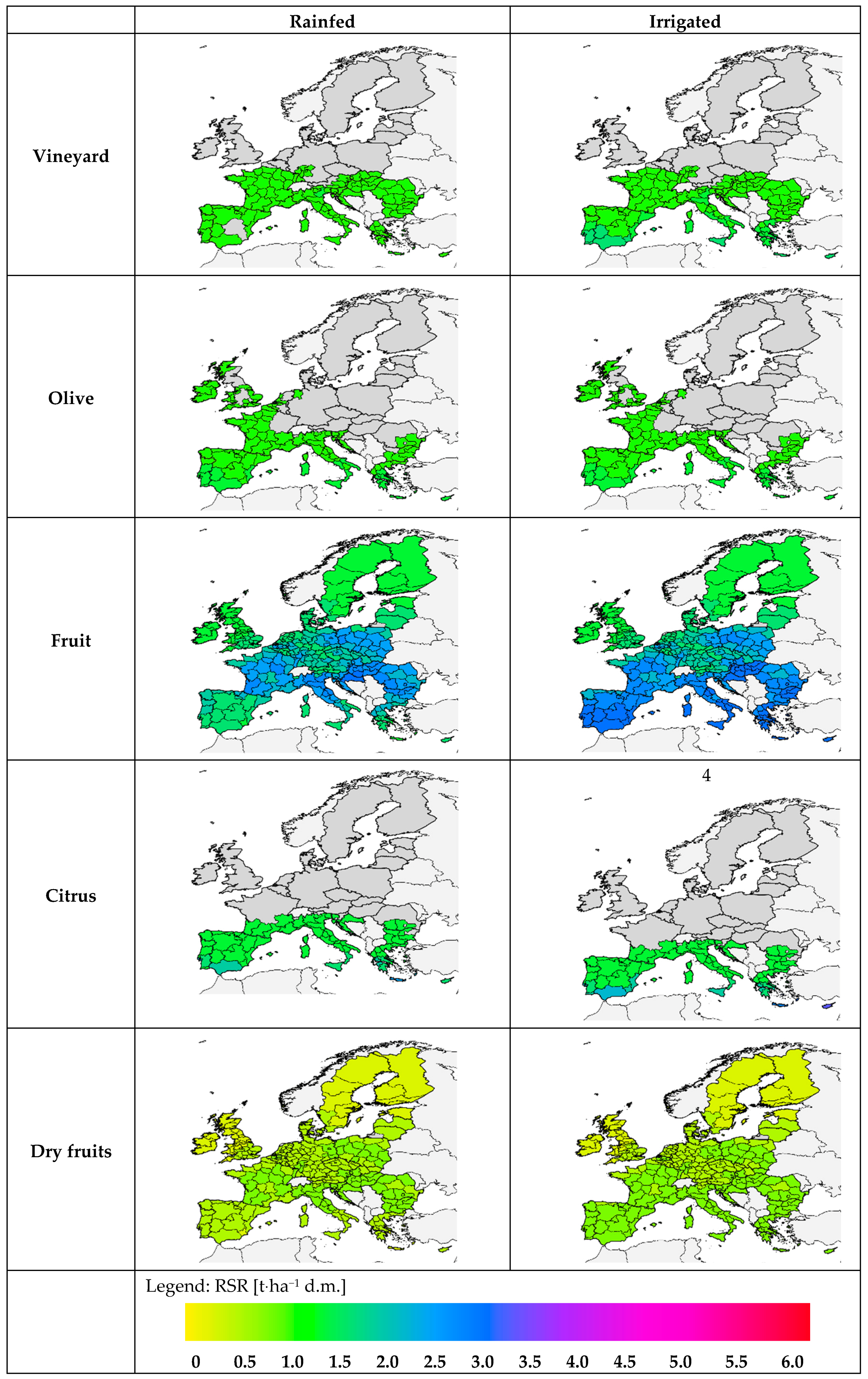
3.6. Spatially Explicit Results

The ramp functions (presented in Table 4) have been utilised to convert the continuous raster coverages of the agroclimatic variables (ACP_Gral_Ab and ECO_wclim) into continuous coverages of RSR (expressed in t/ha d.m.). These results are presented for the five crop groups with maps of the RSR values in form of raster geographical coverages in Figure 5 (see full extent maps in Figure S1). The average RSR values obtained by NUTs2 are presented in Figure 6 (see full extent maps in Figure S2). The numeric results are presented by NUTs0 in Table 4. Additional tables of the average RSR ratios obtained by NUTs2 and NUTs3 are presented in Tables S1 and S2 respectively.
The results in Figure 5 reflect the good ability of the agro-climatic variables to predict the distribution of the suitable zones for crop development in EU28. Notwithstanding, it is evidenced some areas where the models fail, in concrete for the ECOCROP vineyard model. As result, the work provides continuous coverages with RSR values varying according to agro-climatic conditions (in coherence with the results of the correlation analysis summarised in Table 3).
Figure 5 and Figure 6 denote that the most productive crops in terms of pruning production (t·ha−1 d.m.) are citrus and fruit (pome and stone fruits). Olive and vineyard are crops groups which productivity is intermediate, and in general, dry fruit crops are the crops with lower production of pruning residues. The distribution in terms of geography follows the results of the agroclimatic variables on which RSR equations apply (ECO_Wclim and ACP_Gral_ab). Vineyard, citrus and olive are crops more adapted to mild temperate, oceanic and sub-tropical climates, and, as observed in Figure 5, Figure 6 and Table 5 no values are produced for colder climates. In the case of vineyard it is evidenced a limitation of Ecocrop results to reproduce the vineyard varieties adapted to colder areas, since countries like Czech Republic or Poland fail in the prediction. Furthermore the rainfed vineyard distribution (see Figure 5) is quite restrictive, and also shows a limited capacity to predict crop suitability in dry areas where it is actually a viable crop.
This deviation in the model results can be explained from agronomic and ecological reasons. On the one hand vineyard is a species grown under a rich variety of different agronomic practices, and counting with a vast amount of varieties adapted to different climates; on the other hand, vineyard can prosper the dry seasons in areas where special ecological conditions of the soil preserve moisture. This is a shortcoming of Ecocrop, and thus of the results obtained by this work, which shall deserve further continuation. Dry fruits and fruit tree species are quite varied groups which geographical distribution bases on the results of a non-crop specific variable, the ACP_gral_ab. Therefore the distribution of crops in EU28 is quite extended. That should not be observed as an actual foreseen of the suitable zones (as Ecocrop predicts), but as an indication of the agronomic potential. Therefore the present may show RSR potential for nuts or fruits in areas where they are only grown very marginally, or under very special agronomics.
Table 5 incorporates the aggregated results by EU28 country (by NUT0 units) of the country average RSR values for both, rainfed and irrigated cropping. The mean and standard deviation has been obtained by country by applying zonal statistics functions available in QGIS. These values are obtained from the pixel values contained inside each of the EU28 country shapes. Cases where standard deviation is zero occur in countries where all grid cells evaluated have got a unique constant value; this occurs in countries where the crops do not adapt well, and thus the independent variable (ECO_wclim or ACP_Gral_ab) is in all grid cells lower than the lower threshold of the proposed ramp functions—as were described in Table 4. It is worth mentioning that the RSR values resulted in all cases larger or equal under irrigated conditions, than under rainfed, as expected.

4. Conclusions

The main conclusions of the work are as follows:
  • It has been possible to apply a genuine methodology to correlate pruning yields with several influencing factors. This method opens a door for developing new research works able to improve the biomass assessments at large scale by using non-constant biomass productivity ratios.
  • It has been stated a large variability of pruning productivity, as it depends on multiple factors like crop, variety, soil, climate, agronomics, weather during the growing period, pruning method, and multiple human factors.
  • The results of the study showed the existence of a weak to moderate correlation between multiple factors and the pruning productivity.
  • At a large scale climatic factors revealed to correlate better with pruning productivity—RSR, expressed as t·ha−1 of dry matter—and were able to explain a not negligible part of the RSR changeability.
  • RSR average values and ranges have been produced for EU28 countries (NUTs0) and regional units (NUTs2, NUTs3), which is a major contribution of the present work.
  • Notwithstanding the achieved materialisation of results, the authors recommend to consider them as a first piece of the improvement for assessing pruning biomass potentials of agricultural crop species. These equations should be updated and improved in future.
  • The work has revealed the limitations of an indirect data gathering method—published papers and surveys—. Sampling in future works is strongly advised as preferred method to gather data, though it requires much higher efforts and time for achieving a good sample when the territory object of study is large.
The continuity of this work is necessary for improving the reliability of the results and to provide new productivity equations. Widening the size of the sample (currently 230 records) is necessary as it will provide more consistent result. The new incorporated records are advised to be obtained by direct field sampling to reduce uncertainty. Crop variety—denoting plant vigour, and useful for segmentation— and crop yield are two relevant parameters not properly covered in the present work for a substantial part of the database. Crop variety has a strong influence in the productivity of pruning and thus is a crucial part that should be prioritised in any future work to categorise and segmentate—if necessary—the database. Yield has been successfully utilised in previous work to correlate with agricultural residues productivity. It is therefore a must to incorporate it in future works as a measured or surveyed variable, and not as a predicted value from agro-ecological models. As well interviews to farmers or agricultural technicians in charge of the exploitation accompanying the data sampling are encouraged to detect potential influences of human factors, which are argued to be a source of variability not well traced under the current work.

Supplementary Materials

The following are available online at https://www.mdpi.com/1996-1073/12/5/957/s1, Figure S1: Productivity of pruning residue RSR (t·ha−1 d.m.) under rainfed and irrigated (full extent), Figure S2: Productivity of pruning residue RSR (t·ha−1 d.m.) under rainfed and irrigated conditions by NUT2 geographical units (full extent), Table S1: RSR values by NUTs2 in EU28, Table S2: RSR values by NUTs3 in EU28.

Author Contributions

D.G.-G. conceived and designed the research; D.G.-G., A.D. and F.C.V.-C. performed the research; D.G.-G., A.D. and F.C.V.-C. analyzed the data and contributed materials/analysis tools; A.D. and D.G.-G. wrote the paper.

Funding

This research was funded by the European Commission’s Seventh Framework Programme under the grant contract FP7-KBBE-312078, entitled EuroPruning Project (“Development and implementation of a new and non-existent logistics chain for biomass from pruning”). The APC was funded by Wroclaw University of Environmental and Life Science (pro-development sources D210/0021/18).

Acknowledgments

Authors would also like to express their sincere gratitude to all collaborators in the vest data collection: project partners performing data collection, experts, authors of scientific papers and other scientists. A detailed list can be found in EuroPruning report D3.1, available at www.europruning.eu.

Conflicts of Interest

The funders had no role in the design of the study; in the collection, analyses, or interpretation of data; in the writing of the manuscript, or in the decision to publish the results.

References

  1. García, D.; Rezeau, A. Introducción al aprovechamiento energético de biocombustibles sólidos. In Energía de la Biomasa; Sebastian, F., García, D., Rezeau, A., Eds.; Prensas Universitarias de Zaragoza: Zaragoza, Spain, 2010; Volume I, p. 47. ISBN 978-84-92774-91-3. [Google Scholar]
  2. Velazquez-Marti, B. Quantification and inventory of biomass. In Aprovechamiento De La Biomasa Para Uso Energético; Universitat Politècnica de València: Barcelona, Spain, 2017; Volume 4, p. 840. [Google Scholar]
  3. García-Galindo, D.; Pascual, J.; Asin, J.; Garcia-Martín, A. Variability and confidence interval in the estimation of agricultural residual biomass at a municipality level in Teruel province (Spain). In Proceedings of the 15th European Biomass Conference, Berlín, Germany, 7–11 May 2007. [Google Scholar]
  4. Dyjakon, A. Harvesting and Baling of Pruned Biomass in Apple Orchards for Energy Production. Energies 2018, 11, 1680. [Google Scholar] [CrossRef]
  5. Elbersen, B.; Startisky, I.; Hengeveld, G.; Schelhaas, M.-J.; Naeff, H.; Böttcher, H. Atlas of EU Biomass Potentials. Deliverable 3.3: Spatially Detailed and Quantified Overview of EU Biomass Potential Taking into Account the Main Criteria Determining Biomass Availability from Different Sources. 2012. Available online: https://ec.europa.eu/energy/intelligent/projects/sites/iee-projects/files/projects/documents/biomass_futures_atlas_of_technical_and_economic_biomass_potential_en.pdf (accessed on 28 February 2019).
  6. Dees, M.; Höhl, M.; Datta, P.; Forsell, N.; Leduc, S.; Fitzgerald, J.; Verkerk, H.; Zudin, S.; Lindner, M.; Elbersen, B.; et al. A Spatial Data Base on Sustainable Biomass Cost-Supply of Lignocellulosic Biomass in Europe-Methods & Data Sources. Deliverable Report D1.6-S2Biom Project. 2017. Available online: https://www.s2biom.eu/images/Publications/D1.6_S2Biom_Spatial_data_methods_data_sources_Final_Final.pdf (accessed on 28 February 2019).
  7. Elbersen, B.; Forsell, N.; Leduc, S.; Staritsky, I.; Witzke, P.; Ramirez-Almeyda, J. Chapter 2—Existing Modeling Platforms for Biomass Supply in Europe. In Modeling and Optimization of Biomass Supply Chains; Panoutsou, C., Ed.; Academic Press: London, UK, 2017; pp. 25–54. ISBN 978-0-12-812303-4. [Google Scholar]
  8. García-Galindo, D.; Gómez-Palmero, M.; Pueyo, E.; Germer, S.; Pari, L.; Alfano, V.; Dyjakon, A.; Sagarna, J.; Rivera, S.; Poutrin, C. Agricultural pruning as biomass resource: Generation, potentials and current fates. an approach to its state in Europe. In Proceedings of the European Biomass Conference and Exhibition Proceedings; ETA-Florence Renewable Energies, Amsterdam, The Netherlands, 6–9 June 2016; pp. 1579–1595. [Google Scholar]
  9. Scarlat, N.; Martinov, M.; Dallemand, J.-F. Assessment of the availability of agricultural crop residues in the European Union: Potential and limitations for bioenergy use. Waste Manag. 2010, 30, 1889–1897. [Google Scholar] [CrossRef] [PubMed]
  10. Panoutsou, C.; Bauen, A.; Elbersen, B.; Dees, M.G.; Stojadinovic, D.; Glavonjic, B.; Zheliezna, T.; Wenzelides, L.; Langeveld, H. Chapter 1—Biomass Supply Assessments in Europe: Research Context and Methodologies. In Modeling and Optimization of Biomass Supply Chains; Panoutsou, C., Ed.; Academic Press: London, UK, 2017; pp. 1–24. ISBN 978-0-12-812303-4. [Google Scholar]
  11. Pari, L.; Alfano, V.; García-Galindo, D.; Suardi, A.; Santangelo, E. Pruning biomass potential in Italy related to crop agro-climatic conditions. Energies 2018, 11, 1365. [Google Scholar] [CrossRef]
  12. Scarlat, N.; Blujdea, V.; Dallemand, J.-F. Assessment of the availability of agricultural and forest residues for bioenergy production in Romania. Biomass Bioenergy 2011, 35, 1995–2005. [Google Scholar] [CrossRef]
  13. Fischer, G.; Prieler, S.; van Velthuizen, H.; Berndes, G.; Faaij, A.; Londo, M.; de Wit, M. Biofuel production potentials in Europe: Sustainable use of cultivated land and pastures, Part II: Land use scenarios. Biomass Bioenergy 2010, 34, 173–187. [Google Scholar] [CrossRef]
  14. Fischer, G.; Hizsnyik, E.; Prieler, S.; Shah, M.; van Velthuizen, H. Biofuels and Food Security. OFID Study Prepared by IIASA; IIASA—Intenational Institute for Applied Systems Analysis: Vienna, Austria, 2009. [Google Scholar]
  15. Fischer, G.; Hizsnyik, E.; Prieler, S.; van Velthuizen, H. Assessment of Biomass Potentials for Biofuel Feedstock Production in Europe: Methodology and Results; IIASA—International Institute for Applied Systems Analysis, 2007. Available online: https://ec.europa.eu/energy/intelligent/projects/sites/iee-projects/files/projects/documents/refuel_assessment_of_biomass_potentials.pdf (accessed on 28 February 2019).
  16. EUROSTAT. Agricultural Areas of Permanent Crops by NUTs3; European Statistical Data Support (ESDS), 2016. [Google Scholar]
  17. CIRCE. Mapping and Analysis of the Pruning Biomass Potential in Europe. Project Report D3.1. EuroPruning Project (FP7-312078). 2014. Available online: http://www.europruning.eu/web/lists/pubfiles.aspx?type=pubdeliverables (accessed on 28 February 2019).
  18. WUELS. Report on Environmental Evaluation of the Supply Chain. Project Report D8.1. EuroPruning Project (FP7-312078). 2016. Available online: http://www.europruning.eu/web/lists/pubfiles.aspx?type=pubdeliverables (accessed on 28 February 2019).
  19. García-Galindo, D.; Cay Villa-Ceballos, F.; Vila-Villarroel, L.; Pueyo, E.; Sebastián, F. Seeking for Ratios and Correlations from Field Data for Improving Biomass Assessments for Agricultural Pruning in Europe. Methods and Results. In Proceedings of the 24th European Biomass Conference and Exhibition, Amsterdam, The Netherlands, 6–9 June 2016; pp. 214–232, ISBN 978-88-89407-165. [Google Scholar]
  20. Zucaro, A.; Forte, A.; Fierro, A. Life cycle assessment of wheat straw lignocellulosic bio-ethanol fuel in a local biorefinery prospective. J. Clean. Prod. 2018, 194, 138–149. [Google Scholar] [CrossRef]
  21. Searle, S.Y.; Malins, C.J. Waste and residue availability for advanced biofuel production in EU Member States. Biomass Bioenergy 2015, 89, 2–10. [Google Scholar] [CrossRef]
  22. Roberts, J.J.; Cassula, A.M.; Osvaldo Prado, P.; Dias, R.A.; Balestieri, J.A.P. Assessment of dry residual biomass potential for use as alternative energy source in the party of General Pueyrredón, Argentina. Renew. Sustain. Energy Rev. 2015, 41, 568–583. [Google Scholar] [CrossRef]
  23. Montola, V.; Colonna, N.; Alfano, V.; Gaeta, M.; Sasso, S.; De Luca, V.; De Angelis, C.; Soda, A.; Braccio, G. Censimento potenziale energetico biomasse, metodo indagine, atlante Biomasse su WEB-GIS. Ric. Sist. Elettr. 2009, RSE/2009/1, 141. [Google Scholar]
  24. Velázquez-Martí, B.; Fernández-González, E.; López-Cortés, I.; Salazar-Hernández, D.M. Quantification of the residual biomass obtained from pruning of vineyards in Mediterranean area. Biomass Bioenergy 2011, 35, 3453–3464. [Google Scholar] [CrossRef]
  25. Velázquez-Martí, B.; Fernández-González, E.; López-Cortés, I.; Salazar-Hernández, D.M. Quantification of the residual biomass obtained from pruning of trees in Mediterranean olive groves. Biomass Bioenergy 2011, 35, 3208–3217. [Google Scholar] [CrossRef]
  26. Velázquez-Martí, B.; Fernández-González, E.; López-Cortés, I.; Callejón-Ferre, A.J. Prediction and evaluation of biomass obtained from citrus trees pruning. J. Foodagric. Environ. 2013, 11, 1485–1491. [Google Scholar]
  27. Velázquez-Martí, B.; Fernández-González, E.; López-Cortés, I.; Salazar-Hernández, D.M. Quantification of the residual biomass obtained from pruning of trees in Mediterranean almond groves. Renew. Energy 2011, 36, 621–626. [Google Scholar] [CrossRef]
  28. Fernández-Puratich, H.; Oliver-Villanueva, J.V.; Alfonso-Solar, D.; Peñalvo-López, E. Quantification of potential lignocellulosic biomass in fruit trees grown in mediterranean regions. BioResources 2013, 8, 88–103. [Google Scholar] [CrossRef]
  29. Zomer, R.J.; Bossio, D.A.; Trabucco, A.; Yuanjie, L.G. Trees and Water: Smallholder Agroforestry on Irrigated Lands in Northern India. IWMI Research Report 122; International Water Management Institute: Colombo, Sri Lanka, 2007. [Google Scholar]
  30. Zomer, R.J.; Trabucco, A.; Bossio, D.A.; Verchot, L. V Climate change mitigation: A spatial analysis of global land suitability for clean development mechanism afforestation and reforestation. Agric. Ecosyst. Environ. 2008, 126, 67–80. [Google Scholar] [CrossRef]
  31. CGIAR DIVA GIS Software. Ecocrop Module 2012. Available online: www.diva-gis.org (accessed on 12 January 2019).
  32. Fischer, G.; Nachtergaele, F.O.; Prieler, S.; Teixeira, E.; Toth, G.; van Velthuizen, H.; Verelst, L.; Wiberg, D.A. Global Agro-Ecological Zones. Model Documentation. V. 3.0.; FAO-IIASA: Laxenbourg, Austria, 2012. [Google Scholar]
  33. EEA. The Biogeographical Regions Dataset; European Environment Agency: Copenhagen, Denmark, 2011.
  34. Kottek, M.; Grieser, J.; Beck, C.; Rudolf, B.; Rubel, F. World Map of the Köppen-Geiger Climate Classification Updated. 2006, Volume 15. Available online: https://www.schweizerbart.de/papers/metz/detail/15/55034/World_Map_of_the_Koppen_Geiger_climate_classificat (accessed on 28 February 2019).
  35. Cohen, J. Statistical Power Analysis for the Behavioral Sciences, 2nd ed.; Lawrence Erlbaum Associates: New York, NY, USA, 1988; ISBN 0805802835. [Google Scholar]
  36. Cay Villa-Ceballos, F. Elaboración de ratios para la evaluación del potencial de biomasa residual agrícola leñosa; University of Zaragoza: Zaragoza, Spain, 2015. [Google Scholar]
Figure 1. Ramp function utilized for adapting the mathematical expressions found in the regression analysis with RSR (left) and RPR (right) as dependent variable. RSR: Residue to surface ratio; RPR: Residue to product ratio.
Energies 12 00957 g001
Figure 2. Ramp function building from values of segregated whisker plots.
Energies 12 00957 g002
Figure 3. Location of database records in Europe.
Energies 12 00957 g003
Figure 4. Whisker plots obtained by zoning the scatter plots of three crop groups.
Energies 12 00957 g004
Figure 5. Productivity of pruning residue under rainfed and irrigated conditions estimated as surface ratio RSR (t·ha−1 d.m.) for five crop groups.
Energies 12 00957 g005
Figure 6. Productivity of pruning residue under rainfed and irrigated conditions estimated as surface ratio RSR (t·ha−1 d.m.) for five crop groups by NUT2 geographical unit.
Energies 12 00957 g006
Table 1. Summary of variables implemented in the registry of the database, and connection with plant, plantation and agronomical factors.
Type of IndicatorsParameterVar NameExpected Relation (+/−)Factors Represented by the Variable
D: Directly; i: Indirectly; C: Through Calculation; M: Through a Model
Source
SpeciesVarietyAgePhenologyOther Plant PhenologyClimate (ave. T, P, Rad)Weather (Ave T, P, Rad Profiles)Spec. Weather (Season, Yearly T, P)SoilPruning FrequencyCrop FormPlantation DensityIrrigationFertilisationIntensification DegreeOther Plant ManagementNOTES
Crop character-risticsSpecies (Nom/Surv)SPECIESn.a.D Lit/Surv
Crop_group (Nom/Surv)GROUPn.a.D Lit/Surv
Age (Cont/Surv)AGE+ D Lit/Surv
Agrono-mics:Frequency (Disc/Surv)FREQ D Lit/Surv
Tree form (Nom/Surv)FORMn.a. D Lit/Surv
Density (Cont/Surv)DENS+/− D Lit/Surv
Irrigation (Dicot/Surv)IRR+ D Lit/Surv
Intensification (Ord/Class)INT+ CCC Calculated
ClimateEuropean biogeog. regions (Ord/Class)BioGRn.a. ii [33]
Köppen-Geiger (Ord/Class)Koppen+ M [34]
Thermal climate (Ord/Class)ThCLIMn.a. M FAO-IIASA [32]
Length growing period (Cont/Calc)LGP+ C
Global-Aridity index (Cont/Calc)AR_idx+ C C CGIAR-CSI [29,30]
Agro-climatic indicatorsGlobal Potential Evapotranspiration (Cont/Calc)PET_idx+ i C
Reference Evapotranspiration (Cont/Model)ETP+ M M FAO-IIASA [32]
Net primary productivity (Cont/Model)NPP+ M M M
Agro-climatic potential RefCrops (Cont/Model)ACP_ab, ACP_rel+ M M MMMMnce
Suitability of crop species (Cont/Model) ECO_Wclim, ECO_wclim_th, ECO_ccm, ECO_ccm_th+D M M M ECOCROP [31]
Agro-climatic potential of olive (Cont/Model)ACP_OL+D M M MMM FAO-IIASA [32]
Agro-ecological indicatorsAgro-ecologic potential of RefCrops (Cont/Model)AEP_ab, AEP_AG+ M M M MMMMnce
Suitability of crop species (Cont/Model)AEP_rel, AEP_AG_rel, AEP_Sidx, AEP_AG_Sidx+ M M M MMMMnce
Agro-ecologic potential of oliveAEP_OL, AEP_Sidx_OL, AEP_AG_OL, Sidx_OL+D M M M MMM
Crop yieldsGAEZ average agricultural yield (Cont/Model)Ylds_ab, Ylds_rel, Yld_gaps+ D D D DDDDnce
GAEZ olive yield (Cont/Model)Ylds_OL_ab, Yld_gaps_OL+D M M M MMM
Crop yield from field work (Cont/Surv)YLD+DDii iiiiiiiiii Lit/Surv
Table abbreviations: Variable types: Nom: nominal; Dic: Dichotomous; Ord: ordinal; Cont: continuous. Expected relation: +: direct positive relation; −: inverse relation; n.a.: not applicable. Column “Notes”: nce: not crop specific (meaning that it was built as an average of several crops to represent the potentiality of a site, not the potential of any of the targeted crop groups). Source: Lit: literature review and contact with authors of the scientific or technical paper; Surv: survey to experts.
Table 2. Records contained in the database by crop, type of information source, irrigation regime and country.
Database ConfigurationRSR Values (t·ha−1 d.m.)
Crop GroupN SpeciesNr Records Total (Biblio/Survey)N Rfed/N Irr.N CountriesMean (Std.Dev)Min/Max
Vineyard1 (multiple varieties)72 (59/13)56/1661.23 (±0.57)0.11/2.66
Olive1 (multiple varieties)50 (43/7)42/851.34 (±1.15)0.35/5.75
Pome fruit2 (pear/apple of multiple varieties)52 (28/24)27/2562.18 (±1.55)0.06/6.41
Stone fruit4 (peach, apricot, cherry, plum)36 (16/20)23/1371.93 (±1.21)0.30/5.38
Citrus3 (orange, lemon, n.d.)7 (2/5)0/722.33 (±1.89)0.60/5.14
Dry fruit13 (almond, hazelnut, walnut)13 (10/3)10/331.38 (±1.79)0.18/6.93
nd: not determined; Rfed: Rainfed; Irr: Irrigated; d.m.: dry matter.
Table 3. Result of the correlation analysis between RSR (t·ha−1 d.m.) and the agronomic- and climatic-like variables.
CropAgronomic VariableSample SizeConfidence (p-Value)ρSpearmanClimatic VariableSample SizeConfidence (p-Value)ρSpearman
VineyardDensity720.497−0.081Köppen720.0310.254
Age720.063−0.221AR_idx720.490−0.083
Intensification720.0220.269ACP_Gral_ab720.1730.162
ECO_Wclim580.0020.398
OliveDensity500.0210.325Köppen500.0070.377
Age500.8340.030AR_idx500.0170.335
Intensification500.108−0.230ACP_Gral_ab500.4870.101
ECO_Wclim460.5360.094
Pome fruitDensity500.893−0.019Köppen500.258−0.163
Age500.4670.105AR_idx500.046−0.283
Intensification500.3690.130ACP_Gral_ab500.0300.308
ECO_Wclim210.6660.100
Stone fruitDensity380.6970.065Köppen380.2760.181
Age380.0790.289AR_idx380.8150.039
Intensification380.039−0.336ACP_Gral_ab380.064−0.304
ECO_Wclim300.030−0.396
CitrusDensity70.355−0.414Köppen70.9320.040
Age70.645−0.214AR_idx710
Intensification7----ACP_Gral_ab70.180−0.571
ECO_Wclim700.964
NutsDensity130.0410.572Köppen130.5940.163
Age130.855−0.056AR_idx130.6330.147
Intensification130.0980.478ACP_Gral_ab130.0910.488
ECO_Wclim310
Table 4. Ramp functions construction and equations.
CropAgro-Climatic Variable (X axis)Lower Threshold (X; Y)Upper Threshold (X; Y)Equation
Fruit[24] ACP_gral_ab2.0; 1.54.0/2.8Y = (0.4 + 1.3 * X)/2
Dry fruit2.0; 0.54.0/1Y = 0.5 * X/2
Vineyard[25] ECO_wclim20; 1.0560; 1.69Y = 0.733 + 0.016 * X
Citrus20; 1.3260; 5.76Y = −0.898 + 0.111* X
Olive20; 1.180; 1.55Y = (0.45 X + 57)/60
Table 5. Summary of RSR results (t·ha−1 d.m.) by crop group by country in EU28.
EU28Mean (Std dev)
VineyardOliveFruitCitrusNuts
Rfed.Irr.Rfed.Irr.Rfed.Irr.Rfed.Irr.Rfed.Irr.
AT1.05 (0.00)1.05 (0.00)--1.97 (0.51)2.01 (0.55)--0.68 (0.20)0.70 (0.21)
BE--1.10 (0.00)1.10 (0.00)1.94 (0.31)1.97 (0.30)--0.67 (0.12)0.68 (0.12)
BG1.05 (0.00)1.07 (0.04)1.14 (0.02)1.14 (0.02)2.34 (0.35)2.66 (0.37)1.32 (0.00)1.32 (0.00)0.82 (0.14)0.95 (0.14)
CY1.06 (0.02)1.69 (0.00)1.25 (0.05)1.47 (0.07)1.50 (0.00)2.80 (0.00)1.6 (0.51)3.16 (1.01)0.50 (0.00)1.00 (0.00)
CZ----1.82 (0.38)1.87 (0.41)--0.62 (0.15)0.64 (0.16)
DE1.05 (0.00)1.05 (0.00)1.10 (0.00)1.10 (0.00)1.90 (0.32)1.96 (0.35)--0.66 (0.12)0.68 (0.13)
DK----1.55 (0.09)1.57 (0.10)--0.52 (0.03)0.53 (0.04)
EE----1.50 (0.00)1.50 (0.00)--0.50 (0.00)0.50 (0.00)
EL1.09 (0.10)1.51 (0.27)1.28 (0.09)1.30 (0.11)1.78 (0.27)2.76 (0.18)1.62 (0.55)1.74 (0.68)0.61 (0.10)0.99 (0.07)
ES1.09 (0.10)1.32 (0.29)1.25 (0.08)1.26 (0.09)1.67 (0.26)2.65 (0.34)1.51 (0.41)1.67 (0.64)0.57 (0.10)0.94 (0.13)
FI----1.50 (0.00)1.50 (0.00)--0.50 (0.00)0.50 (0.00)
FR1.07 (0.08)1.11 (0.16)1.15 (0.06)1.15 (0.07)2.16 (0.41)2.31 (0.50)4.08 (2.00)4.72 (1.87)0.75 (0.16)0.81 (0.19)
HR1.09 (0.09)1.10 (0.13)1.19 (0.06)1.19 (0.06)2.61 (0.37)2.64 (0.37)1.32 (0.00)1.32 (0.00)0.93 (0.14)0.94 (0.14)
HU1.05 (0.00)1.06 (0.01)--2.65 (0.14)2.80 (0.04)--0.94 (0.05)1.00 (0.01)
IE--1.10 (0.01)1.10 (0.01)1.50 (0.00)1.50 (0.00)--0.50 (0.00)0.50 (0.00)
IT1.14 (0.13)1.26 (0.23)1.23 (0.10)1.23 (0.10)2.18 (0.51)2.66 (0.36)1.38 (0.23)1.43 (0.36)0.76 (0.19)0.95 (0.14)
LT----1.57 (0.05)1.63 (0.06)--0.53 (0.02)0.55 (0.02)
LU----1.60 (0.18)1.64 (0.24)--0.54 (0.07)0.55 (0.09)
LV----1.50 (0.02)1.52 (0.04)--0.50 (0.01)0.51 (0.01)
MT1.14 (0.05)1.69 (0.00)1.39 (0.01)1.46 (0.01)2.19 (0.07)2.80 (0.00)1.79 (0.16)3.97 (0.27)0.77 (0.03)1.00 (0.00)
NL--1.10 (0.00)1.10 (0.00)1.63 (0.18)1.66 (0.17)--0.55 (0.07)0.56 (0.07)
PL----2.24 (0.31)2.29 (0.32)--0.79 (0.12)0.80 (0.12)
PT1.14 (0.18)1.52 (0.25)1.31 (0.09)1.31 (0.09)1.77 (0.24)2.77 (0.14)1.6 (0.37)1.62 (0.40)0.60 (0.09)0.99 (0.04)
RO1.05 (0.00)1.06 (0.02)1.10 (0.01)1.10 (0.01)2.36 (0.49)2.53 (0.49)1.32 (0.00)1.32 (0.00)0.83 (0.19)0.90 (0.19)
SE----1.50 (0.01)1.50 (0.02)--0.50 (0.00)0.50 (0.01)
SL1.07 (0.04)1.07 (0.03)1.13 (0.03)1.13 (0.03)2.34 (0.52)2.37 (0.51)1.32 (0.00)1.32 (0.00)0.82 (0.20)0.83 (0.20)
SK1.05 (0.00)1.05 (0.00)--2.14 (0.50)2.23 (0.56)--0.75 (0.19)0.78 (0.21)
UK--1.10 (0.00)1.10 (0.00)1.51 (0.03)1.52 (0.05)--0.50 (0.01)0.51 (0.02)

