Forecasting the Carbon Price Using Extreme-Point Symmetric Mode Decomposition and Extreme Learning Machine Optimized by the Grey Wolf Optimizer Algorithm

Abstract

Due to the nonlinear and non-stationary characteristics of the carbon price, it is difficult to predict the carbon price accurately. This paper proposes a new novel hybrid model for carbon price prediction. The proposed model consists of an extreme-point symmetric mode decomposition, an extreme learning machine, and a grey wolf optimizer algorithm. Firstly, the extreme-point symmetric mode decomposition is employed to decompose the carbon price into several intrinsic mode functions and one residue. Then, the partial autocorrelation function is utilized to determine the input variables of the intrinsic mode functions, and the residue of the extreme learning machine. In the end, the grey wolf optimizer algorithm is applied to optimize the extreme learning machine, to forecast the carbon price. To illustrate the superiority of the proposed model, the Hubei, Beijing, Shanghai, and Guangdong carbon price series are selected for the predictions. The empirical results confirm that the proposed model is superior to the other benchmark methods. Consequently, the proposed model can be employed as an effective method for carbon price series analysis and forecasting.

1. Introduction

With the growing concern about climate change, many countries and regions have begun to adopt the carbon emission trading mechanism to effectively control greenhouse gas emissions [1]. The carbon trading market, playing a significant role in dealing with global climate change, is one of the most effective tools [2,3]. As one of the largest carbon emitters [4], China officially proposed to implement an initial carbon emissions trading system in 2010, which was response to the challenge of climate change. Subsequently, seven pilot provinces and cities were set up, including Beijing, Shanghai, Guangdong, Shenzhen, Tianjin, Chongqing, and Hubei in 2011. Afterwards, carbon emissions trading platforms were launched during 2013 and 2014. Furthermore, on December 19, 2017, the national emissions trading scheme (ETS) was officially implemented [5], which almost doubled the coverage of the carbon pricing system [6]. To date, the Chinese government has established eight pilot carbon markets that have valid developments for reducing greenhouse gas emissions [7]. In addition, by the end of December 2018, the cumulative trading volume pilot exceeded 270 million tons, and the total turnover exceeded 6 billion yuan. Obviously, China is the world’s largest energy consumer and greenhouse gas emitter [8]. The ETS has become an extremely significant financial market, and accordingly, it will play an increasingly important role in reducing emissions in the future accordingly.

Currently, the carbon price covers about 20% of greenhouse gas emissions [9], and calls for a global carbon price are intensifying [10,11]. Economists believe that carbon pricing is one of the most effective ways to reduce global warming emissions [12]. Carbon pricing is greatly relevant today, and it will be even more so in the future. Hence, it is necessary to predict the carbon price, to understand the evolutionary process of the carbon price. On the one hand, for policy makers, forecasting carbon price accurately is conducive to grasping the price fluctuations of carbon market, which can formulate carbon emission trading market policies and develop a reasonable carbon price mechanism. Specifically, to stabilize the price, and to promote the rational development of the market, the policy makers could adjust the price range of the price and the quantity of the market stability reserve, according to the law of carbon price changes [13]. On the other hand, for investors, predicting carbon price accurately can provide scientific decision-making tools and guide investors towards to make reasonable investments. Consequently, it makes sense to integrate carbon price predictions.

According to existing literature, researchers have paid great attention to carbon price analysis: research for on-the-spot and futures prices of EU ETS [14,15,16,17,18], studies on the relationship between the carbon price and the energy price [19,20,21,22,23], and research into the market efficiency based on the carbon price [24,25,26,27]. Although some achievements have been made with existing carbon price analysis, the literature on carbon price prediction is limited [28]. Currently, there are two main representative theories in carbon price forecasting: factor forecasting and time series forecasting. Factor forecasting, mainly based on different factors, has a good performance. The coal, oil, natural gas, other energy prices, and global equity indices are exogenous variables, which are applied to forecast carbon price [29,30]. However, influencing factors are exogenous variables, which results in errors, and the failure of carbon price prediction.

Time-series forecasting, which includes econometric and statistical prediction models, artificial intelligence models and ensemble models, is mainly based on the historical data, using price-only to predict. Econometric and statistical prediction models, as traditional classical prediction methods, are widely used in the traditional carbon market for carbon price forecasting and fluctuation analysis. These models mainly include the generalized autoregressive conditional heteroscedasticity model (GARCH), the autoregressive conditional heteroscedasticity model (ARCH), dynamic model averaging (DMA), etc. Byun and Cho [31] put forward GARCH-type models to forecast European Climate Exchange (ECX) carbon futures from December 2008 to December 2011, and concluded that the GJR-GARCH [32] model performs better than the TGARCH and GARCH models. The AR-GARCH model was adopted by Chevallier to predict the second-stage carbon price fluctuations of the EU ETS, which illustrated that the proposed model had a high prediction accuracy [33]. Furthermore, the nonparametric model was conducted to forecast the Blue Next spot and ECX futures prices from April 2005 to April 2010. The result illustrated that the error of nonparametric modeling is lower than the linear autoregressive models [34]. Moreover, Conrad et al. [35] regarded fractionally integrated asymmetric power GARCH (FIAPGARCH) as a predicted model, to predict the first- and second-phase carbon prices of EU ETS, and determined that the FIAPGARCH model can describe the fluctuation of carbon price well. María et al. [36] executed the autoregressive moving average including exogenous covariates and generalized autoregressive conditional heteroskedasticity model (ARMAX-GARCH) framework with a time-varying jump probability, to forecast the price of Phase 2 EU price, and concluded that the ARMAX-GARCH framework with a time-varying jump probability is more accurate than the ARMAX-GARCH model. Also, dynamic model averaging (DMA) was conducted by Koop et al. to forecast the carbon markets, which confirmed that DMA can perform forecasting accurately [37]. Although the econometric and statistical prediction models can obtain higher precisions in carbon market price predictions, they are based on the fact that the carbon market price changes are highly nonlinear and non-stationary. In addition, it is difficult to effectively deal with nonlinear modes that are hidden in the prices of non-stationary carbon markets, so that they generally cannot obtain satisfactory prediction results.

To overcome the limitations of the econometric and statistical prediction models, the artificial intelligence algorithms demonstrating excellent nonlinear modeling capabilities, as represented by artificial neural network (ANN) and least-squares support regression (LSSVR), were selected to predict the carbon price. Tsai and Kuo [38] constructed an Ant-Based Radial Basis Function Network (ARBFN) to predict carbon price based on the Radial Basis Function Network (RBFN), and Ant Colony Optimization (ACO), which provided an accurate and real-time method for the forecasting of carbon price. Zhu and Wei [39], presented several hybrid models of autoregressive integrated moving average model (ARIMA) and least square support vector machine (LSSVM) to predict the carbon futures prices of EU ETS from April 2005 to March 2011, and concluded that the model ARIMALSSVM2 exceeded the single ARIMA, ANN, and LSSVM models. Also, a novel hybrid neuro-fuzzy controller model, based on an ANN system and an adaptive neuro-fuzzy inference system (ANFIS), was provided by Atsalakis to predict the carbon futures price, which was superior to other models such as ARIMA, ANN, ARIMALSSVM2, etc., in terms of forecasting accuracy [40]. Fan et al. [41] examined the multilayer perceptron (MLP) neural network for forecasting carbon price. The results indicated that the model showed good performance in forecasting the carbon price. Zhang et al. [28] employed the grey neural network (GNN), optimized by the ant colony algorithm (ACA) model to forecast the carbon spot price of EU ETS. The results indicated that the model performed better than signal ARIMA, ANN, and LSSVM.

Based on the aforementioned discussion, it is manifest that some models were optimized by using other algorithms such as the ACO, ACA, and ANN systems. Nevertheless, these methods have high requirements for the accuracy and smoothness of historical data, which have defects for non-stationary data with time-varying properties. In addition, the artificial intelligence models neglect the information of different features in the original carbon price time series, which affects the accuracy of prediction. Considering that the original carbon price time series characteristics are unstable and random, the signal decomposing technique was introduced into carbon price forecasting.

Currently, to achieve the goal of eliminating the carbon price stochastic volatility, researchers generally examine the empirical mode decomposition (EMD) or ensemble empirical mode decomposition (EEMD) to analyze the time series. Several studies have proven the efficiencies of these algorithms. Zhu et al. [42] came up with a multiscale ensemble forecasting model that integrated empirical mode decomposition (EMD), genetic algorithm (GA), and ANN, to predict the carbon price, which demonstrated that the multiscale ensemble forecasting model outperformed the ANN and GAANN models. Sun et al. [43] proposed a combined forecasting model based on variational mode decomposition (VMD) and spiking neural networks (SNNs), and confirmed that the models have high accuracies and reliabilities. Taking four futures prices of EU ETS as sample, Zhu et al. [44] successfully introduced an EMD-based evolutionary least squares support vector regression model, and concluded that the model was suitable for nonlinear and non-stationary carbon price forecasting. In addition, the EMD model, and the LSSVM model with a kernel function prototype and particle swarm optimization (PSO), were integrated to forecast the daily carbon future prices for the EU ETS during December 2015 and 2016. The results confirmed that the proposed model had high levels of accuracy [3]. Furthermore, Feng et al. [45] applied the EEMD to analyze the carbon price of the EU ETS, to improve forecasting accuracy and reliability.

However, despite of the good performance of multiscale ensemble forecasting models, based on EMD/VMD/EEMD, there are drawbacks to ameliorate. Consequently, the ensemble empirical mode decomposition (ESMD) is a further improvement of the EMD, which overcomes the outcomes of EMD. First, the ESMD method solves the problem of mode mixing for the EMD method, which can enhance the effectiveness of decomposition. In addition, ESMD uses the direct interpolation (DI) method, which can accurately reflect the fluctuation characteristics and the trend changes of the time series. Moreover, ESMD can adaptively time–frequency decomposition, based on time-series local time-varying features, which are highly suitable for analyzing non-stationary and nonlinear time series.

Furthermore, it is crucial to note that the extreme learning machine (ELM) has been widely executed in various forecasting fields successfully, such as in short-term load forecasting [46], the sub-component load forecasting [47], short term electricity price forecasting [48], and wind speed forecasting [49]. However, for the ELM model, the input weight matrix and the hidden layer deviation are randomly determined, so that the nodes of some hidden layers fail or cannot meet the data requirements. Thus, it becomes crucial to select the optimal number of hidden-layer nodes adaptively. Therefore, Abdoos [50] applied the Gram–Schmidt orthogonalization (GSO), to optimize the ELM in order to forecast the wind power of two wind farms. Rocha et al. [51] proposed the PSO to optimize the ELM to predict the distributed electrical generation system capacity. Sun et al. [52] focused on the PSO-ELM to predict carbon price, and the results indicated that PSO-ELM performed better. Based on these, this paper employs the grey wolf optimizer algorithm (GWO) to optimize the ELM. Also, this paper could prove the applicability of this method in carbon price prediction.

From the above, this paper puts forward a hybrid forecasting approach with ESMD, a partial autocorrelation function (PACF), ELM, and GWO. Also, the carbon price series of China, such as Hubei, Beijing, Shanghai, and Guangdong are selected as the samples. Firstly, considering the characteristics of the carbon price series, the ESMD is employed to decompose the carbon price time series into a finite and small number of intrinsic mode functions (IMFs) and one residue. Decomposing the original time series by ESMD can effectively determine the characteristic information of the original data. Secondly, the PACF is applied to determine the input variables of each subsequence. Also the ELM optimized by the GWO is utilized to forecast the decomposed components. Furthermore, in order to verify the effectiveness and the practicability of the proposed method, this paper compares the forecasting results of the proposed method with other benchmark methods, and demonstrates that the proposed method can achieve a high prediction accuracy. Hence, it is effective to predict the carbon price with nonlinearity and non-stationarity.

The contributions of this paper may be concluded as follows:

• The extreme-point symmetric mode decomposition is applied, to decompose the carbon price to promote the prediction accuracy.
• The extreme learning machine optimized by the grey wolf algorithm could obtain a good performance with predictions.
• The proposed model ESMD-GWO-ELM significantly improves the forecasting accuracy of the carbon price, with only the historical carbon price sequence being taken into account.

The remainder of this paper is structured as follows: Section 2 describes the extreme-point symmetric mode decomposition, the extreme learning machine, the grey wolf optimizer algorithm, and the partial autocorrelation function. Section 3 introduces the proposed model: ESMD-GWO-ELM. The empirical analysis and forecasting results are discussed in Section 4. Finally, conclusions are drawn in Section 5.

2. Methodology

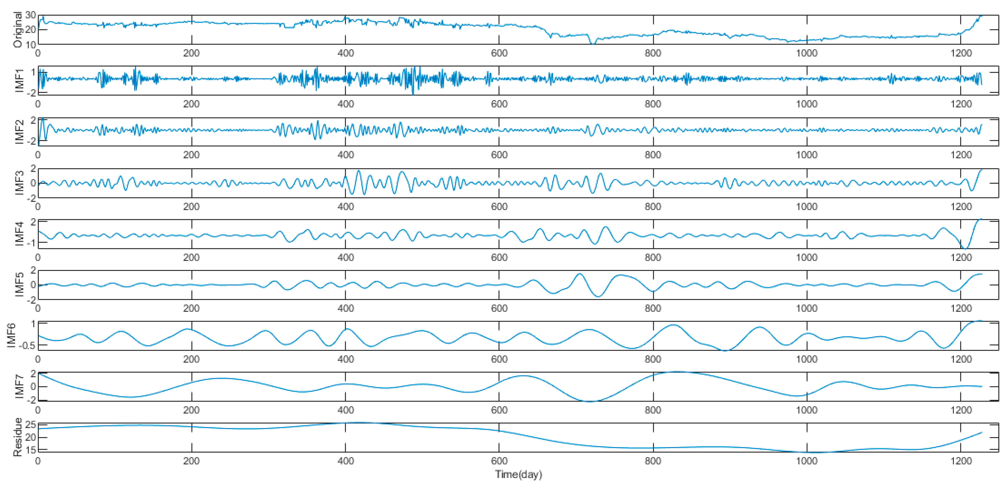
2.1. Extreme-Point Symmetric Mode Decomposition

Extreme-point symmetric mode decomposition (ESMD), a new method for the empirical mode decomposition method, features an improved and optimized version of EMD [53]. The ESMD method solves the problems of screening termination and modal aliasing in the EMD method. Moreover, the ESMD method draws on the idea of EMD, and changes the external envelope interpolation into internal pole-symmetric interpolation. This borrows from the idea of the least squares, to optimize the last residual modality to make it become the global adaptive mean of the entire data, and to determine the optimal number of filters. In addition, considering that all integral transforms, including the Hilbert transform, have inherent defects in analyzing time-frequency changes, ESMD abandons the traditional concept of spectrum analysis relying on integral transform, and creatively proposes a direct interpolation (DI) method, which intuitively reflects the time-varying amplitude and frequency of each mode.

The ESMD method consists of two parts: the first part is the mode decomposition, which can generate several intrinsic mode functions (IMFs) and one optimal adaptive global averaging. The second part is the time–frequency analysis, using the direct interpolation method to calculate the instantaneous frequency of the natural mode, which analyzes frequency changes on each time scale, and determines when mutations will occur at each time scale. The specific steps of ESMD are shown as follows:

Step 1:

Find all of the extreme points (maximum and minimum) of the whole data series $X$, and record as $E_i\left(1\le i\le n\right)$.

Step 2:

Connect all of the adjacent poles with line segments, and record the midpoints of the line as $F_i\left(1\le i\le n-1\right).$

Step 3:

The boundary points $F_0$ and $F_n$ are added to the left and right ends, respectively, using certain methods.

Step 4:

Construct $p$ interpolation curves $L_1,\cdots ,L_p\left(p\ge 1\right)$ by using the obtained $n+1$ midpoints, and calculate the mean curve $L^{*}=\left(L_1+\cdots +L_P\right)/p$.

Step 5:

Repeat the above steps for the series $X-L^{*}$ until the number of screenings reaches the preset maximum value $K$, and the first decomposed empirical mode is obtained and named as $M_1$.

Step 6:

Repeat the above five steps for the remaining sequence $X-M_1$ until the remaining sequence $\mathrm{R}$ has only a certain number of poles left, and the decomposed empirical modes $M_2,M_3\cdots$ can be obtained, respectively.

Step 7:

Change the number of screening times $K$ within the limited interval $\left[K_{min},K_{max}\right]$, repeat the above six steps, and then calculate the variance ratio $\mathsf{\sigma }/{\sigma }_0$ and plot the variance ratio graph with $K$.

Step 8:

Select the number of transformations $K_0$ as the optimal number of screenings when the variance ratio $\mathsf{\sigma }/{\sigma }_0$ is the smallest, and repeat the previous six steps until all of the decomposed empirical modes are outputs.

After decomposition, the original time series $X$ can be expressed as $X=\sum M_i+R$; that is, the time series X is decomposed into a series of empirical modes and one residual variable.

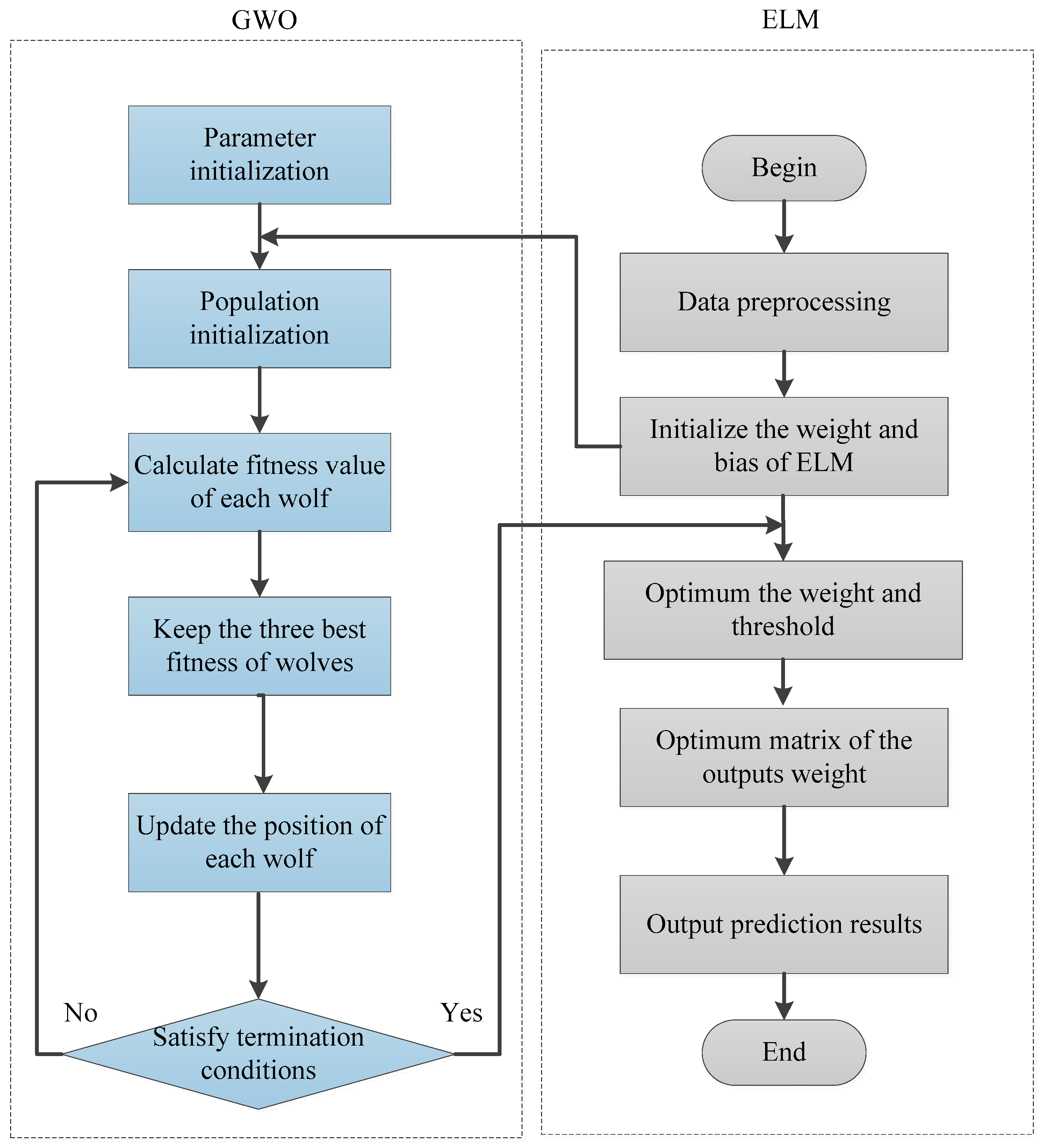
2.2. Extreme Learning Machine

The extreme learning machine (ELM), proposed by Huang et al, is a new type of single hidden layer feedforward neural network (SLFN) learning algorithm [54]. The ELM algorithm is comprised of an input layer, a hidden layer, and an output layer, which randomly generates the connection weights of the input layer, the hidden layer, and the threshold of the hidden layer neurons. Moreover, there is no need to adjust during the training process, and a unique optimal solution can be obtained once the number of neurons is set in the hidden layer requirements. Compared with the traditional neural network method, the algorithm has the advantages of a fast learning speed, less human intervention, and a strong generalization ability.

The output of an ELM is as follows:

$$f\left(x\right)={\displaystyle \sum }_{i=1}^N{\beta }_{i}G\left(a_i,b_i,x\right)=\beta ·h\left(x\right)$$

(1)

where $h\left(x\right)=\left[G\left(a_1,b_1,x_1\right),\cdots ,G\left(a_N,b_N,x_N\right)\right]$ is the output vector for the hidden layer relative to the input $x$, ${\beta }_i$ is the output weight of the $i$th hidden layer node and the output neuron; $a_i$ is the input weight for the input neurons and $i$th hidden layer node; $b_i$ is the threshold of the $i$th hidden layer node.

Then, the output weight can be obtained by solving the least-squares solution of the linear Equation (2).

$$\min {\displaystyle \sum }_{i=1}^N\Vert \beta ·h\left(x_i\right)-y_i\Vert$$

(2)

The least squares solution of Equation (2) is:

$$\beta =H^{+}Y$$

(3)

where $H^{+}$ is the Moore–Penrose-generalized inverse of the hidden layer output matrix $H$ [55], which is used to calculate the matrices of the hidden layer. ELM aims to minimize the training errors and the norm of the output weights.

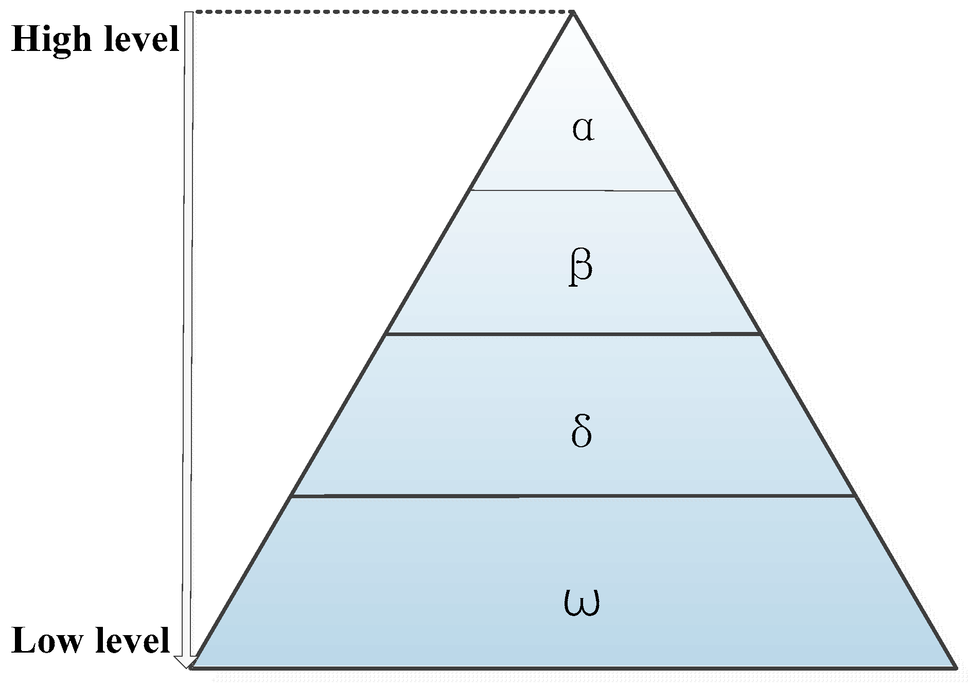
2.3. Grey Wolf optimizer Algorithm

The grey wolf algorithm (GWO) is a new group of intelligence algorithms recently proposed by Mirjalili et al. [56], which simulate the hierarchy and hunting behavior of grey wolves in nature, and finds the optimal value. The GWO algorithm exhibits more advantages in terms of fast convergence and less adjustment parameters in solving function optimization problems.

The social ranks of the grey wolves are divided into four parts: alpha (α), beta (β), delta (δ), and omega (ω) as in Figure 1. The hunting behaviors of the wolves mainly involve tracking and approaching the prey, tracking the prey, and attacking the prey.

$\mathsf{\alpha }$ stands for the head wolf, which leads the grey wolf group, followed by $\mathsf{\beta }$, which assists the head wolf in making decisions; $\mathsf{\delta }$ are the ordinary wolves commanded by $\mathsf{\alpha }$ and $\mathsf{\beta }$, and the underlying wolf is $\mathsf{\omega }$ is commanded by $\mathsf{\alpha }$, $\mathsf{\beta }$, and $\mathsf{\delta }$. Under the leadership of $\mathsf{\alpha }$, the group of grey wolves captures the prey, and the wolves gradually approach and track the prey by scent and other information. The wolves surround the prey once the location of the prey is determined.

During surrounding of the prey, the distance between the grey wolf and the prey are shown in Equations (4) and (5):

$$\overrightarrow{D}=\left|\overrightarrow{C}·{\overrightarrow{X}}_{P\left(t\right)}-\overrightarrow{X}\left(t\right)\right|$$

(4)

$$\overrightarrow{X}\left(t+1\right)={\overrightarrow{X}}_{P\left(t\right)}-\overrightarrow{A}·\overrightarrow{D}$$

(5)

where $t$ represents the iterations, ${\overrightarrow{X}}_{P\left(t\right)}$ stands for the prey position after the $t$-th iteration, and $\overrightarrow{X}\left(t\right)$ indicates the position of a wolf. $\overrightarrow{D}$ refers to the distance between the grey wolf and the prey, and $\overrightarrow{A}$ and $\overrightarrow{C}$ are the convergence factor and the swing factor, respectively. The calculation formula is shown in Equations (6) and (7):

$$\overrightarrow{A}=2\overrightarrow{a}{\overrightarrow{r}}_1-\overrightarrow{a}$$

(6)

$$\overrightarrow{C}=2{\overrightarrow{r}}_2$$

(7)

where $\overrightarrow{r_1}$ and $\overrightarrow{r_2}$ are random variables between $\left[0,1\right];$ with the number of iterations increases, the convergence factor $\overrightarrow{a}$ decreases linearly from 2 to 0. The optimization process of the GWO algorithm is to locate the prey position based on the positions of $\mathsf{\alpha }$, $\mathsf{\beta }$, and $\mathsf{\delta }$. The $\mathsf{\omega }$ wolves pursue the prey under the guidance of the $\mathsf{\alpha }$, $\mathsf{\beta }$, and $\mathsf{\delta }$ wolves, and they re-determine the prey position according to the best positions of the $\mathsf{\alpha }$, $\mathsf{\beta }$ and $\mathsf{\delta }$ wolves. The positions of the grey wolf group are in accordance with Equation (8) to Equation (14):

$${\overrightarrow{D}}_{\alpha }=\left|{\overrightarrow{C}}_1·{\overrightarrow{X}}_{\alpha }-\overrightarrow{X}\right|$$

(8)

$${\overrightarrow{D}}_{\beta }=\left|{\overrightarrow{C}}_2·{\overrightarrow{X}}_{\beta }-\overrightarrow{X}\right|$$

(9)

$${\overrightarrow{D}}_{\delta }=\left|{\overrightarrow{C}}_3·{\overrightarrow{X}}_{\delta }-\overrightarrow{X}\right|$$

(10)

$${\overrightarrow{X}}_1={\overrightarrow{X}}_{\alpha }-{\overrightarrow{A}}_1·{\overrightarrow{D}}_{\alpha }$$

(11)

$${\overrightarrow{X}}_2={\overrightarrow{X}}_{\beta }-{\overrightarrow{A}}_2·{\overrightarrow{D}}_{\beta }$$

(12)

$${\overrightarrow{X}}_3={\overrightarrow{X}}_{\delta }-{\overrightarrow{A}}_3·{\overrightarrow{D}}_{\delta }$$

(13)

$$\overrightarrow{X}\left(t+1\right)=\frac{{\overrightarrow{X}}_1+{\overrightarrow{X}}_2+{\overrightarrow{X}}_3}{3}$$

(14)

where ${\overrightarrow{X}}_{\alpha }$, ${\overrightarrow{X}}_{\beta }$, and ${\overrightarrow{X}}_{\delta }$ are the positions of $\mathsf{\alpha }$, $\mathsf{\beta }$, and $\mathsf{\delta }$, respectively; ${\overrightarrow{C}}_1$, ${\overrightarrow{C}}_2$ and ${\overrightarrow{C}}_3$ are the random swing factors; ${\overrightarrow{X}}_1$, ${\overrightarrow{X}}_2$, and ${\overrightarrow{X}}_3$ indicate the directions and distances of $\mathsf{\omega }$ wolf towards $\mathsf{\alpha }$, $\mathsf{\beta }$, and $\mathsf{\delta }$. The steps of the GWO algorithm are briefly shown in Algorithm 1.

Algorithm 1: The GWO algorithm

Step 1: randomly initialize the population to be within the specified range; Step 2: calculate the fitness of each individual; Step 3: select, in order of fitness $\mathsf{\alpha }$, $\mathsf{\beta }$, and $\mathsf{\delta }$; Step 4: update the other wolves using formulas (4) to (14) Step 5: update the parameters $\overrightarrow{\mathsf{\alpha }}$, $\overrightarrow{A}$, and $\overrightarrow{C}$; Step 6: if the end condition is not met, go to step 2; Step 7: output the location of the $\mathsf{\alpha }$ wolf.

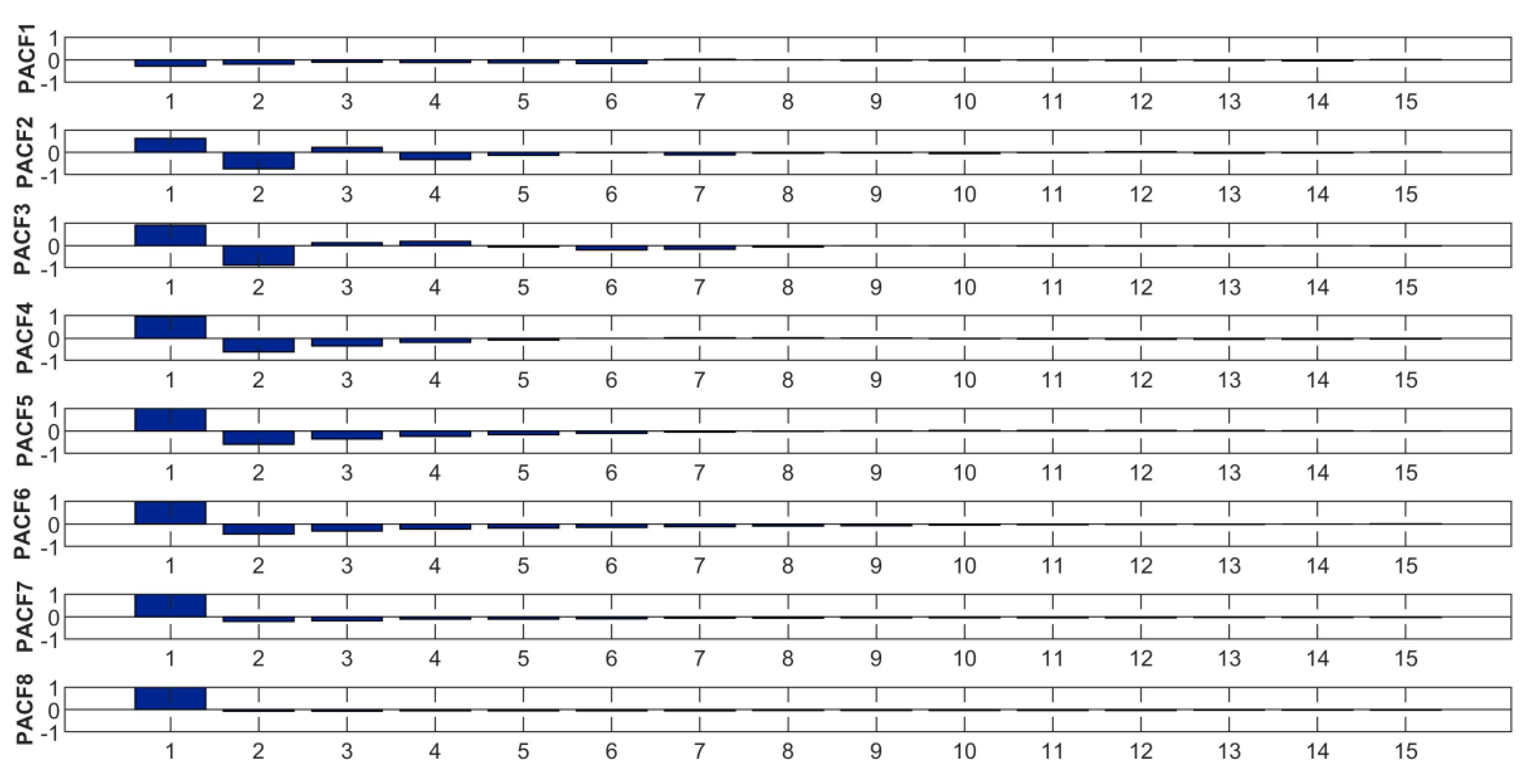
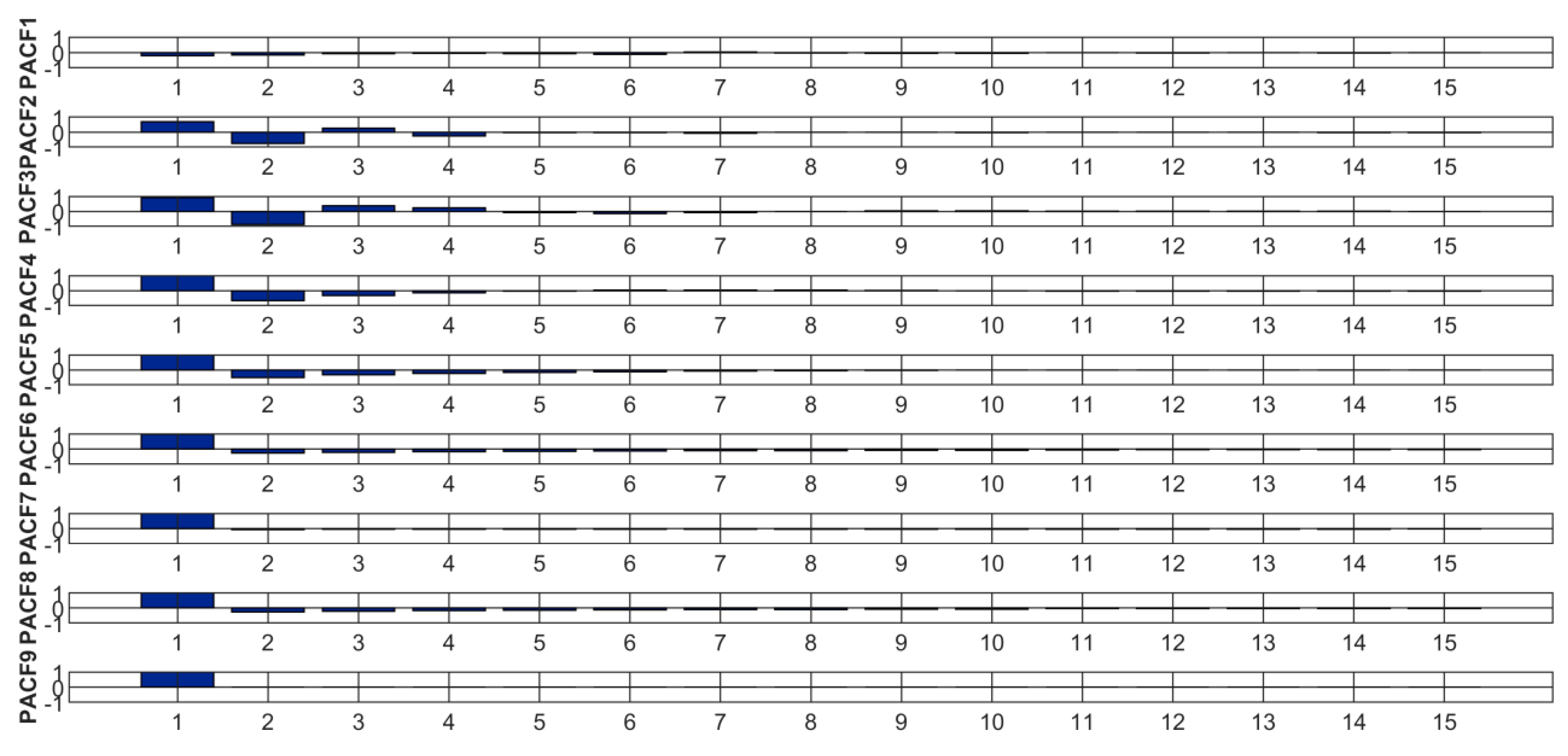
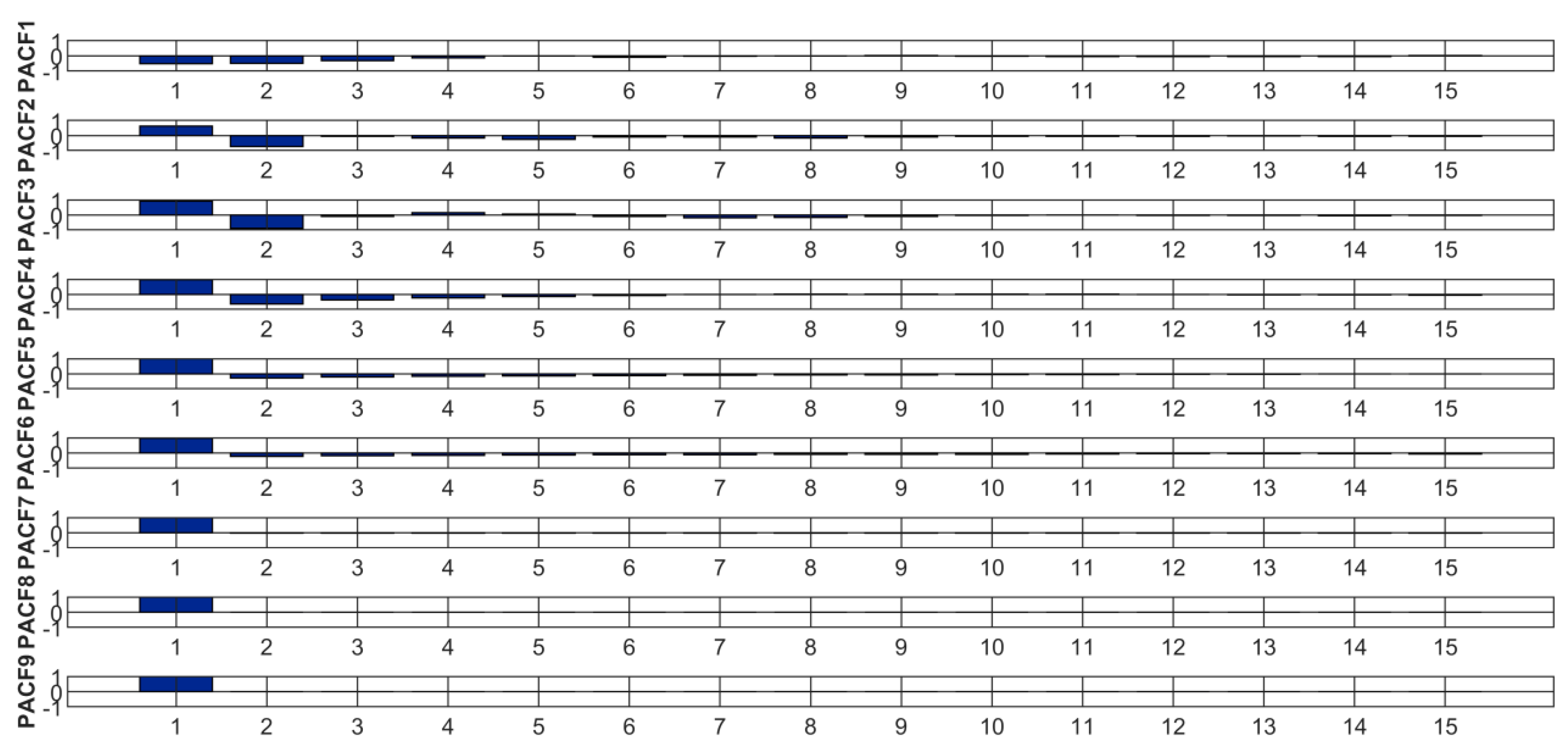
2.4. The Partial Autocorrelation Function

The partial autocorrelation function (PACF), as a common statistical tool, gives the relation that exists between the time series and their lags, which are used to determine the input variables of the neural network [57].

Give a time series $x_t$, with ${\mathsf{Ф}}_{kj}$ representing the $j$ regression coefficient with the $k$-order autoregressive equation, then the k-order autoregressive model is expressed as:

$$x_t={\mathsf{Ф}}_{k1}{x}_{t-1}+{\mathsf{Ф}}_{k2}{x}_{t-2}+\cdots +{\mathsf{Ф}}_{kk}{x}_{t-k}+{\mu }_t$$

(15)

where ${\mathsf{Ф}}_{kk}$ is the last coefficient and the partial autocorrelation function.

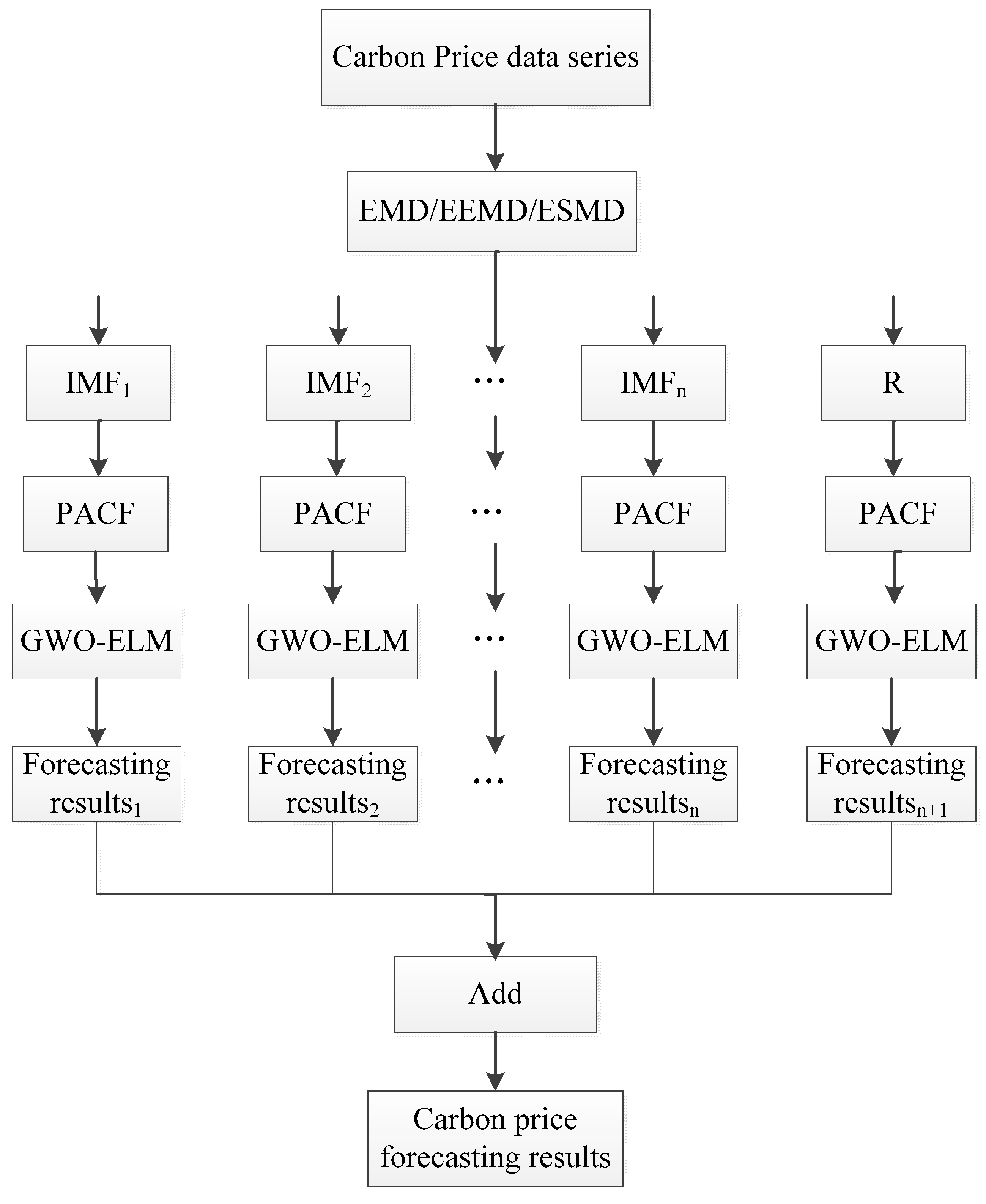
3. The Proposed Model

Figure 2 illustrates the process of the extreme learning machine optimized by the grey wolf optimizer algorithm (GWO-ELM) model. The left part is the GWO algorithm, and the right part is the prediction process of the ELM algorithm. It is apparent that the GWO algorithm is employed to optimize the parameters in ELM, which benefit in obtaining the optimal network.

Figure 3 is the forecasting framework for carbon price, with the ESMD-GWO-ELM model. As can be seen, the original carbon price series is decomposed into several IMFs, and one residue by EMD, EEMD and ESMD at first. Then, the partial autocorrelation function (PACF) is utilized to determine the input variables of each subsequence, so that the series are divided into the training set and test set. Thirdly, the GWO-ELM is employed to predict each series. Finally, the prediction results are compared with the real carbon price.

4. Empirical Analysis

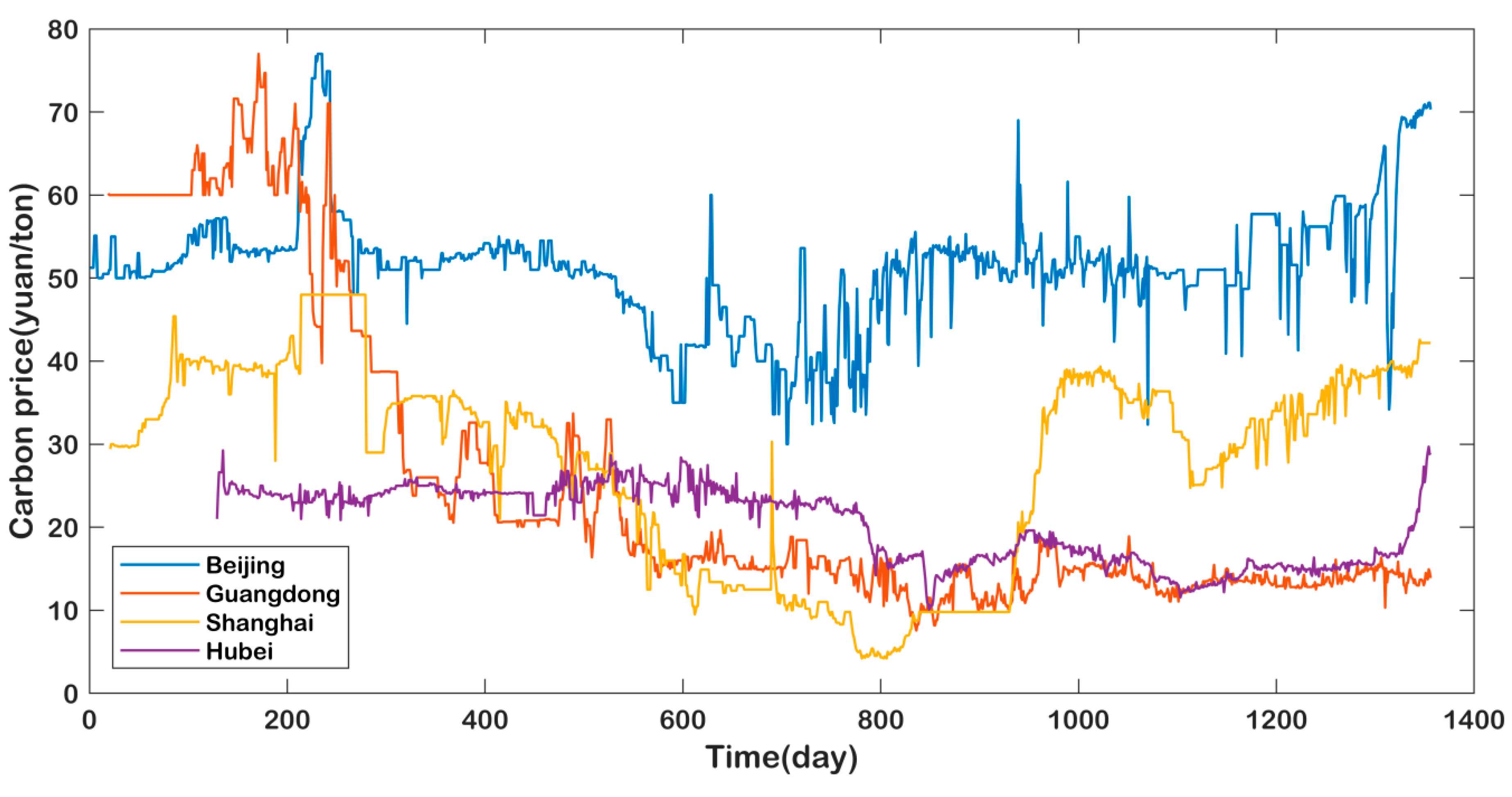
4.1. Data

At present, China has established eight regional carbon trading markets, including Beijing, Shanghai, Guangdong, Shenzhen, Hubei, Fujian, Chongqing, and Tianjin. Among them, Hubei is the world’s third-largest emissions trading system [58]. In addition, Hubei’s carbon emission trading market has the highest degree of liquidity, and the volume is first-ranked [59]. Furthermore, the Hubei pilot emission trading market has been a pioneer among all of pilots, as it owns sufficient transaction data [60]. Hence, Hubei was selected as a sample to forecast the carbon price. In addition, considering the rich volume, the value of carbon trading, and the long transaction time, Beijing, Shanghai, and Guangdong were also selected as examples in this paper [60,61]. The daily data are collected in China’s carbon emissions trading website [62]. The Hubei sample covers the period from 2 April 2014 until 14 August 2018, with 1228 total data points, excluding public holidays. The carbon prices in the Shanghai and Guangdong markets, both from 19 December 2013 until 14 August 2018, and the carbon prices of Beijing from 28 November 2013 until 14 August 2018. The price fluctuations of original carbon price series are shown in Figure 4. From it, it is evident that carbon price series of the four markets were non-stationary and nonlinear.

The data series were divided into two parts: the training sample and the test sample. There are several methods of segmenting the data to train and test the whole data. Generally, most studies classify data for training and assessment based on convenience. In this paper, data is split using a ratio equal to 70:30. Consequently, taking Hubei as an example, my 860 data points are selected as training sets, and the remaining 368 data points are applied, to evaluate the established models. The samples of carbon price are shown in

Table 1. Samples of carbon price.

Carbon Price	Sample	Size	Data
Hubei	Sample set	1228	2014/4/02–2018/8/14
	Training set	860	2014/4/02–2017/2/15
	Testing set	368	2017/2/15–2018/8/14
Beijing	Sample set	1356	2013/11/28–2018/8/14
	Training set	950	2013/12/19–2016/12/13
	Testing set	406	2016/12/14–2018/8/14
Guangdong	Sample set	1338	2013/12/19–2018/8/14
	Training set	937	2013/12/19–2016/12/26
	Testing set	401	2016/12/27–2018/8/14
Shanghai	Sample set	1336	2013/12/19–2018/8/14
	Training set	935	2013/12/19–2016/12/21
	Testing set	401	2016/12/22–2018/8/14

.

The data statistical descriptions of the carbon price series are stated in

Table 2. Statistical descriptions of the carbon price.

Carbon Price	Means	Median	Standard Deviation	Skewness	Kurtosis	Jarque-Bera
Hubei	20.31	22.13	4.48	0.22	1.59	111.24
Beijing	51.33	51.48	7.05	0.33	5.13	282.07
Guangdong	25.57	15.99	18.21	1.34	3.26	406.02
Shanghai	27.91	31.91	12.11	0.46	1.99	103.05

. From this, the carbon price of Beijing had the highest average price, which reached 51.33 RMB. The average prices of Shanghai and Guangdong were lower, at 27.91 and 25.57 RMB, respectively. Also, the average price of Hubei was the lowest, at 20.31 RMB. These four carbon price series were not subject to strict normal distribution. Compared with the normal distribution, the skewnesses of all the four carbon price series are bigger than 0, indicating that the series exhibits positive skewness, which implies that the carbon price series are flatter to the right. The kurtoses of Hubei and Shanghai were both lower than 3, which indicates that these two carbon price series have thin tails, compared to a normal distribution, while the other two cities have fat tails. The Jarque–Bera test, rejecting the null hypothesis that obeys the standard normal distribution at any significant level, further confirms these results, given that this paper tests the non-stationary and nonlinear aspects of the carbon price series.

4.2. Non-Stationary and Nonlinear Tests of Carbon Price

The ADF (Augmented Dicky–Fuller) test is an effective method to test the stability of time series, and the BDS (Brock–Decher–Scheikman) test can effectively detect the nonlinear characteristics of the time series. The size of the embedding dimension $\mathrm{m}$ of the phase space reconstruction in the BDS test generally $m\in \left[2,5\right]$. This paper selects Eviews 8.0 software (Quantitative Micro Software, Irvine, CA, USA) to check the stability and nonlinearity of the carbon price. The test results are shown in

Table 3. ADF test results.

Carbon Price	Stat	Prob.	Stationarity
Hubei	−0.5880	0.9791	×
Beijing	−2.6140	0.2741	×
Guangdong	−2.3184	0.4230	×
Shanghai	−1.5097	0.8262	×

Note: The Stat means statistics. The Prob. indicates that the probability. × indicates that the ADF test of the carbon market price is non-stationary at the 10% significance level.

and

Table 4. BDS test results.

Carbon Price	M-Dimensional Space								Linearity
	2		3		4		5
	Stat	Prob.	Stat	Prob.	Stat	Prob.	Stat	Prob.
Hubei	0.1790	0.0012	0.3084	0.0019	0.3985	0.0022	0.4604	0.0023	×
Beijing	0.1686	0.0031	0.2844	0.0049	0.3612	0.0059	0.4101	0.0061	×
Guangdong	0.2042	0.0028	0.3486	0.0045	0.4500	0.0053	0.5212	0.0056	×
Shanghai	0.1986	0.0015	0.3375	0.0024	0.4333	0.0029	0.4996	0.0030	×

Note: The Stat means statistics. The Prob. indicates that the probability. × shows that the carbon price is nonlinear at a significance level of 1%.

. Apparently, all of the four carbon price series are non-stationary and nonlinear. Taking Hubei carbon price as an example, the ADF test implies that the p-value of Hubei’s carbon market price is greater than 10%, which means that the carbon price is non-stationary at the 10% significance level. The BDS test displays that the carbon price has a p-value of lower than 0.01, indicating that Hubei’s carbon market price is non-linear at the 1% significance level.

4.3. Data Processing

From above, the results illustrated that the original carbon price fluctuation is severe. In order to reduce the interference of noise, the ESMD was utilized to decompose the carbon price into IMFs and residue. To reduce repetition, this paper only gives a detailed description of the carbon price forecast of the Hubei carbon market. The decomposition results after ESMD are illustrated in Figure 5, where the original carbon price series are decomposed into seven IMFs and one residue. These decomposed IMFs exhibited simpler structures, more stable fluctuations, and greater regularity, all of which led to better fitting and forecasting accuracies, as compared with an original carbon price.

Moreover, to demonstrate the excellence of ESMD, EMD and EEMD were employed to decompose the original carbon price series as well. Figure 6 and Figure 7 illustrate the results, respectively. Both EMD and EEMD decomposed the carbon prices into eight IMFs and one residue.

4.4. Determination of the Input Variables by PACF

To overcome the limitations of ignoring the relationship between the inputs and outputs of the model, it is vital to know the relations between the series and their lags. The statistical tool, namely the partial autocorrelation function (PACF), is effective for describing the characteristics of the series [63,64], which are applied toward determining the input variables.

The results of the Hubei carbon prices, decomposed by ESMD, EMD, and EEMD are illustrated in Figure 8, Figure 9 and Figure 10 respectively. Specifically, assuming that $x_t$ is the output variable, ${\mathrm{x}}_{\mathrm{t}-\mathrm{k}}$ is one of the input variables if the partial autocorrelation at lag $\mathrm{k}$ exceeds the approximate 95% confidence interval.

Table 5. The PACF results of the Hubei carbon price.

ESMD		EMD		EEMD
IMFs and R	Lag	IMFs and R	Lag	IMFs and R	Lag
IMF1	(${\mathrm{x}}_{\mathrm{t}-1}$, ${\mathrm{x}}_{\mathrm{t}-2}$, ${\mathrm{x}}_{\mathrm{t}-3}$, ${\mathrm{x}}_{\mathrm{t}-4}$, ${\mathrm{x}}_{\mathrm{t}-5}$, ${\mathrm{x}}_{\mathrm{t}-6}$)	IMF1	(${\mathrm{x}}_{\mathrm{t}-1}$, ${\mathrm{x}}_{\mathrm{t}-2}$, ${\mathrm{x}}_{\mathrm{t}-3}$, ${\mathrm{x}}_{\mathrm{t}-4}$, ${\mathrm{x}}_{\mathrm{t}-5}$, ${\mathrm{x}}_{\mathrm{t}-6}$)	IMF1	(${\mathrm{x}}_{\mathrm{t}-1}$, ${\mathrm{x}}_{\mathrm{t}-2}$, ${\mathrm{x}}_{\mathrm{t}-3}$, ${\mathrm{x}}_{\mathrm{t}-4}$, ${\mathrm{x}}_{\mathrm{t}-5}$, ${\mathrm{x}}_{\mathrm{t}-6}$)
IMF2	(${\mathrm{x}}_{\mathrm{t}-1}$, ${\mathrm{x}}_{\mathrm{t}-2}$, ${\mathrm{x}}_{\mathrm{t}-3}$, ${\mathrm{x}}_{\mathrm{t}-4}$, ${\mathrm{x}}_{\mathrm{t}-5}$, ${\mathrm{x}}_{\mathrm{t}-6}$, ${\mathrm{x}}_{\mathrm{t}-7}$)	IMF2	(${\mathrm{x}}_{\mathrm{t}-1}$, ${\mathrm{x}}_{\mathrm{t}-2}$, ${\mathrm{x}}_{\mathrm{t}-3}$, ${\mathrm{x}}_{\mathrm{t}-4}$, ${\mathrm{x}}_{\mathrm{t}-5}$, ${\mathrm{x}}_{\mathrm{t}-6}$, ${\mathrm{x}}_{\mathrm{t}-7}$)	IMF2	(${\mathrm{x}}_{\mathrm{t}-1}$, ${\mathrm{x}}_{\mathrm{t}-2}$, ${\mathrm{x}}_{\mathrm{t}-3}$, ${\mathrm{x}}_{\mathrm{t}-4}$,${\mathrm{x}}_{\mathrm{t}-5}$, ${\mathrm{x}}_{\mathrm{t}-6}$, ${\mathrm{x}}_{\mathrm{t}-7}$, ${\mathrm{x}}_{\mathrm{t}-8}$, ${\mathrm{x}}_{\mathrm{t}-9}$, ${\mathrm{x}}_{\mathrm{t}-10}$)
IMF3	(${\mathrm{x}}_{\mathrm{t}-1}$, ${\mathrm{x}}_{\mathrm{t}-2}$, ${\mathrm{x}}_{\mathrm{t}-3}$, ${\mathrm{x}}_{\mathrm{t}-4}$, ${\mathrm{x}}_{\mathrm{t}-5}$, ${\mathrm{x}}_{\mathrm{t}-6}$, ${\mathrm{x}}_{\mathrm{t}-7}$, ${\mathrm{x}}_{\mathrm{t}-8}$)	IMF3	(${\mathrm{x}}_{\mathrm{t}-1}$, ${\mathrm{x}}_{\mathrm{t}-2}$, ${\mathrm{x}}_{\mathrm{t}-3}$, ${\mathrm{x}}_{\mathrm{t}-4}$, ${\mathrm{x}}_{\mathrm{t}-5}$, ${\mathrm{x}}_{\mathrm{t}-6}$, ${\mathrm{x}}_{\mathrm{t}-7}$)	IMF3	(${\mathrm{x}}_{\mathrm{t}-1}$, ${\mathrm{x}}_{\mathrm{t}-2}$, ${\mathrm{x}}_{\mathrm{t}-3}$, ${\mathrm{x}}_{\mathrm{t}-4}$, ${\mathrm{x}}_{\mathrm{t}-5}$, ${\mathrm{x}}_{\mathrm{t}-6}$, ${\mathrm{x}}_{\mathrm{t}-7}$, ${\mathrm{x}}_{\mathrm{t}-8}$, ${\mathrm{x}}_{\mathrm{t}-9}$)
IMF4	(${\mathrm{x}}_{\mathrm{t}-1}$, ${\mathrm{x}}_{\mathrm{t}-2}$, ${\mathrm{x}}_{\mathrm{t}-3}$, ${\mathrm{x}}_{\mathrm{t}-4}$, ${\mathrm{x}}_{\mathrm{t}-5}$)	IMF4	(${\mathrm{x}}_{\mathrm{t}-1}$, ${\mathrm{x}}_{\mathrm{t}-2}$, ${\mathrm{x}}_{\mathrm{t}-3}$, ${\mathrm{x}}_{\mathrm{t}-4}$)	IMF4	(${\mathrm{x}}_{\mathrm{t}-1}$, ${\mathrm{x}}_{\mathrm{t}-2}$, ${\mathrm{x}}_{\mathrm{t}-3}$, ${\mathrm{x}}_{\mathrm{t}-4}$, ${\mathrm{x}}_{\mathrm{t}-5}$, ${\mathrm{x}}_{\mathrm{t}-6}$)
IMF5	(${\mathrm{x}}_{\mathrm{t}-1}$, ${\mathrm{x}}_{\mathrm{t}-2}$, ${\mathrm{x}}_{\mathrm{t}-3}$, ${\mathrm{x}}_{\mathrm{t}-4}$, ${\mathrm{x}}_{\mathrm{t}-5}$, ${\mathrm{x}}_{\mathrm{t}-6}$, ${\mathrm{x}}_{\mathrm{t}-7}$)	IMF5	(${\mathrm{x}}_{\mathrm{t}-1}$, ${\mathrm{x}}_{\mathrm{t}-2}$, ${\mathrm{x}}_{\mathrm{t}-3}$, ${\mathrm{x}}_{\mathrm{t}-4}$, ${\mathrm{x}}_{\mathrm{t}-5}$, ${\mathrm{x}}_{\mathrm{t}-6}$, ${\mathrm{x}}_{\mathrm{t}-7}$, ${\mathrm{x}}_{\mathrm{t}-8}$)	IMF5	(${\mathrm{x}}_{\mathrm{t}-1}$, ${\mathrm{x}}_{\mathrm{t}-2}$, ${\mathrm{x}}_{\mathrm{t}-3}$, ${\mathrm{x}}_{\mathrm{t}-4}$, ${\mathrm{x}}_{\mathrm{t}-5}$, ${\mathrm{x}}_{\mathrm{t}-6}$, ${\mathrm{x}}_{\mathrm{t}-7}$, ${\mathrm{x}}_{\mathrm{t}-8}$, ${\mathrm{x}}_{\mathrm{t}-9}$, ${\mathrm{x}}_{\mathrm{t}-10}$)
IMF6	(${\mathrm{x}}_{\mathrm{t}-1}$, ${\mathrm{x}}_{\mathrm{t}-2}$, ${\mathrm{x}}_{\mathrm{t}-3}$, ${\mathrm{x}}_{\mathrm{t}-4}$, ${\mathrm{x}}_{\mathrm{t}-5}$, ${\mathrm{x}}_{\mathrm{t}-6}$, ${\mathrm{x}}_{\mathrm{t}-7}$, ${\mathrm{x}}_{\mathrm{t}-8}$, ${\mathrm{x}}_{\mathrm{t}-9}$, ${\mathrm{x}}_{\mathrm{t}-10}$)	IMF6	(${\mathrm{x}}_{\mathrm{t}-1}$, ${\mathrm{x}}_{\mathrm{t}-2}$, ${\mathrm{x}}_{\mathrm{t}-3}$, ${\mathrm{x}}_{\mathrm{t}-4}$, ${\mathrm{x}}_{\mathrm{t}-5}$, ${\mathrm{x}}_{\mathrm{t}-6}$, ${\mathrm{x}}_{\mathrm{t}-7}$, ${\mathrm{x}}_{\mathrm{t}-8}$, ${\mathrm{x}}_{\mathrm{t}-9}$, ${\mathrm{x}}_{\mathrm{t}-10}$)	IMF6	(${\mathrm{x}}_{\mathrm{t}-1}$, ${\mathrm{x}}_{\mathrm{t}-2}$, ${\mathrm{x}}_{\mathrm{t}-3}$, ${\mathrm{x}}_{\mathrm{t}-4}$, ${\mathrm{x}}_{\mathrm{t}-5}$, ${\mathrm{x}}_{\mathrm{t}-6}$, ${\mathrm{x}}_{\mathrm{t}-7}$, ${\mathrm{x}}_{\mathrm{t}-8}$, ${\mathrm{x}}_{\mathrm{t}-9}$, ${\mathrm{x}}_{\mathrm{t}-10}$)
IMF7	(${\mathrm{x}}_{\mathrm{t}-1}$, ${\mathrm{x}}_{\mathrm{t}-2}$, ${\mathrm{x}}_{\mathrm{t}-3}$, ${\mathrm{x}}_{\mathrm{t}-4}$, ${\mathrm{x}}_{\mathrm{t}-5}$, ${\mathrm{x}}_{\mathrm{t}-6}$, ${\mathrm{x}}_{\mathrm{t}-7}$, ${\mathrm{x}}_{\mathrm{t}-8}$, ${\mathrm{x}}_{\mathrm{t}-9}$, ${\mathrm{x}}_{\mathrm{t}-10}$)	IMF7	(${\mathrm{x}}_{\mathrm{t}-1}$, ${\mathrm{x}}_{\mathrm{t}-2}$, ${\mathrm{x}}_{\mathrm{t}-3}$, ${\mathrm{x}}_{\mathrm{t}-4}$, ${\mathrm{x}}_{\mathrm{t}-5}$)	IMF7	(${\mathrm{x}}_{\mathrm{t}-1}$)
Residue	(${\mathrm{x}}_{\mathrm{t}-1}$, ${\mathrm{x}}_{\mathrm{t}-2}$, ${\mathrm{x}}_{\mathrm{t}-3}$, ${\mathrm{x}}_{\mathrm{t}-4}$)	IMF8	(${\mathrm{x}}_{\mathrm{t}-1}$, ${\mathrm{x}}_{\mathrm{t}-2}$, ${\mathrm{x}}_{\mathrm{t}-3}$, ${\mathrm{x}}_{\mathrm{t}-4}$, ${\mathrm{x}}_{\mathrm{t}-5}$, ${\mathrm{x}}_{\mathrm{t}-6}$, ${\mathrm{x}}_{\mathrm{t}-7}$, ${\mathrm{x}}_{\mathrm{t}-8}$, ${\mathrm{x}}_{\mathrm{t}-9}$, ${\mathrm{x}}_{\mathrm{t}-10}$)	IMF8	(${\mathrm{x}}_{\mathrm{t}-1}$)
		Residue	(${\mathrm{x}}_{\mathrm{t}-1}$)	Residue	(${\mathrm{x}}_{\mathrm{t}-1}$)

presents the PACF results of the Hubei carbon price after ESMD, EMD, and EEMD.

4.5. Accuracy Assessment

In order to evaluate the multi-frequency combined prediction performance proposed in this paper, the root mean square error (RMSE), the mean absolute percentage error (MAPE), and the coefficient of determination (R²) were applied, to measure the prediction accuracies of the proposed models. Among them, apart from the R², the lower the value was, the better the forecasting accuracy of the model was. The R² value ranged from $\left[0,1\right]$ the closer to 1, the better the model.

The calculation formula for these indicators is shown in

Table 6. The calculation formula.

Name	The Calculation Formula
RMSE	$\mathrm{RMSE}=\sqrt{\frac{1}{n}{\displaystyle {\displaystyle \sum }_{t=1}^n}{\left(y_t-{\widehat{y}}_t\right)}^2}$
MAPE	$\mathrm{MAPE}=\frac{1}{n}{\displaystyle {\displaystyle \sum }_{t=1}^n}\left(\frac{y_t-{\widehat{y}}_t}{y_t}\right)\times 100\%$
R2	${\mathrm{R}}^2=\frac{{\left(n\sum {\widehat{y}}_t{y}_t-\sum {\widehat{y}}_t\sum y_t\right)}^2}{\left(n\sum {\widehat{y}}_t{}^2-{\left(\sum {\widehat{y}}_t\right)}^2\right)\left(n\sum y_t{}^2-{\left(\sum y_t\right)}^2\right)}$

. $y_t$ is the real value at time $t$; ${\widehat{y}}_t$ is the prediction for the same period $t$, and $n$ is the number of the training sample.

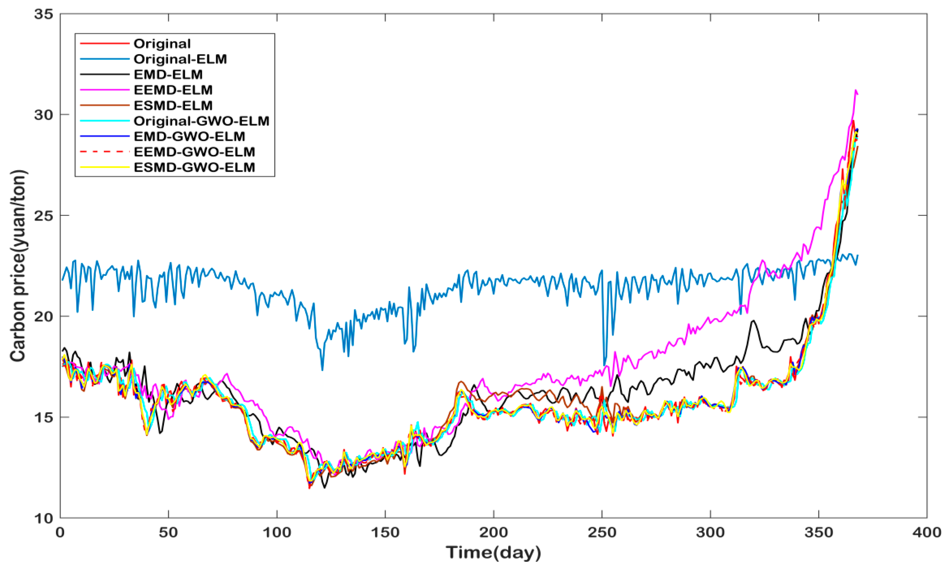
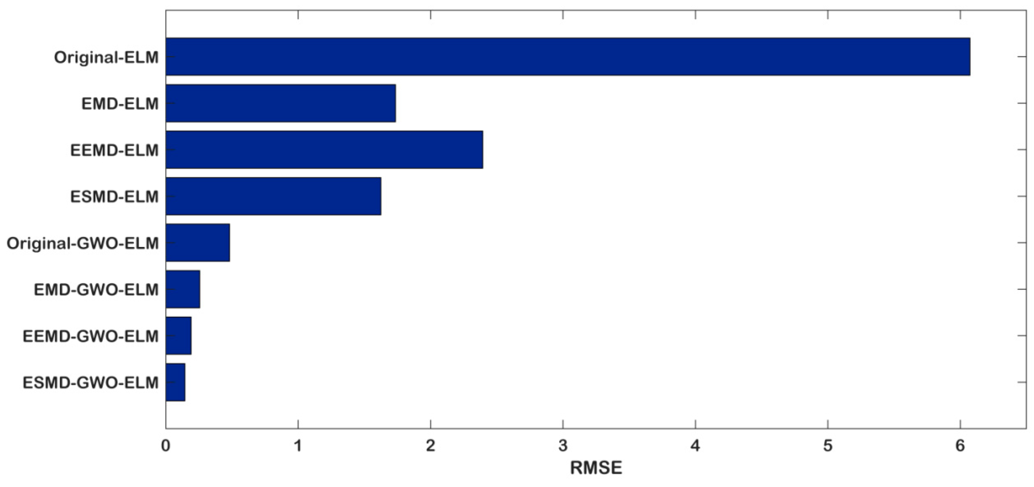
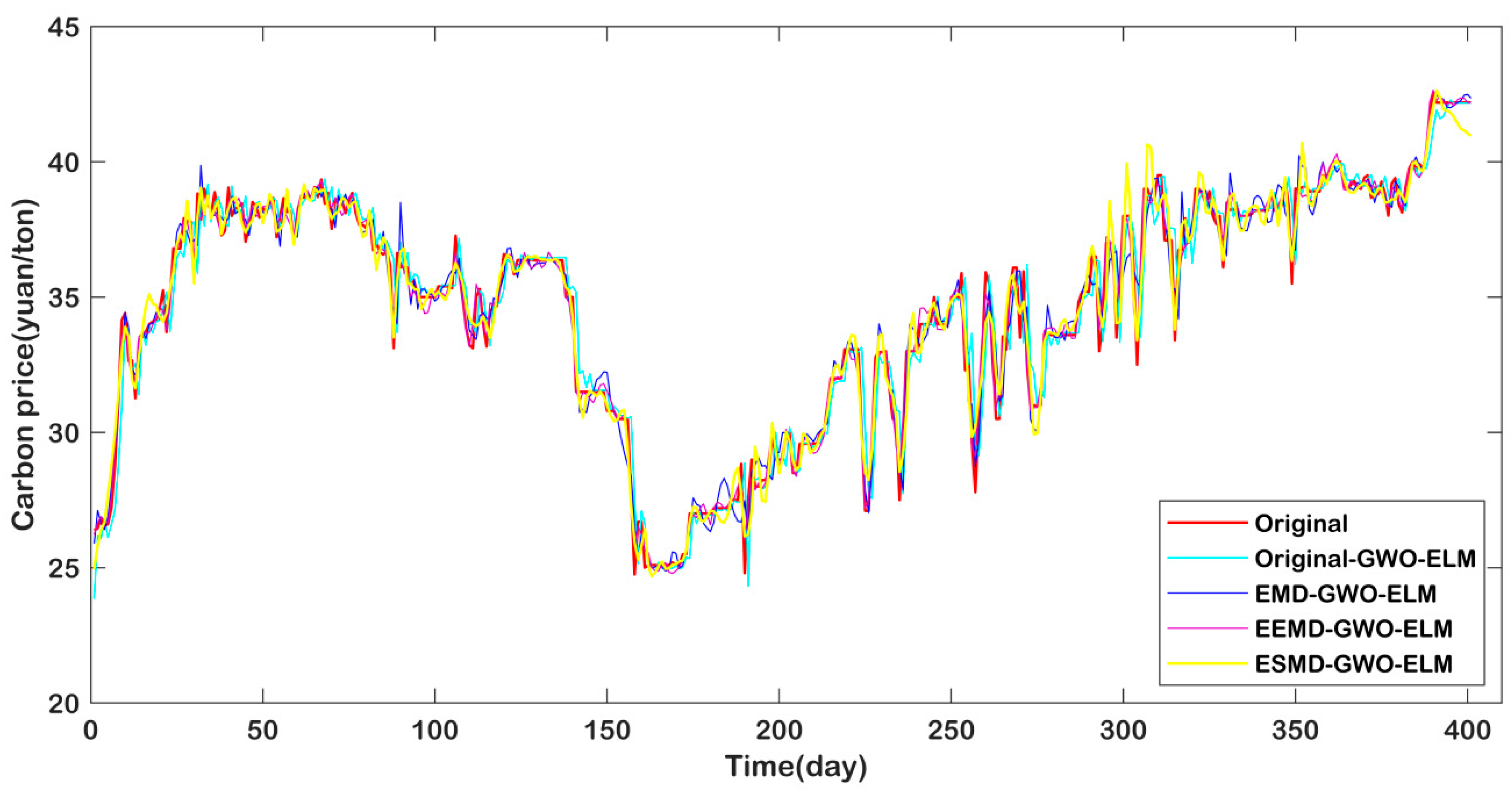
4.6. Forecasting Results and Discussion

In this study, the ESMD-GWO-ELM model was employed to forecast the carbon price. In order to prove the performance forecasting of this model, the benchmark models, including Original-ELM, EMD-ELM, EEMD-ELM, ESMD-ELM, Original-GWO-ELM, EMD-GWO-ELM, and EEMD-GWO-ELM were also provided for predicting the carbon price. All of the models were established in Matlab software (2018, MathWorks, Natick, MA, USA).

The forecasting results are shown in Figure 11; the comparisons of between RMSE, MAE, MAPE, and R² between the eight models are shown in

Table 7. Comparison of the performance of Hubei carbon price forecasting.

Model	RMSE	MAPE (%)	R2
Original-ELM	6.0734	38.42	0.6304
EMD-ELM	1.7352	3.51	0.5761
EEMD-ELM	2.3936	9.92	0.6627
ESMD-ELM	1.6237	2.70	0.6695
Original-GWO-ELM	0.4808	1.98	0.9709
EMD-GWO-ELM	0.2559	1.18	0.9876
EEMD-GWO-ELM	0.1917	1.66	0.9882
ESMD-GWO-ELM	0.1438	0.31	0.9918

and Figure 12, Figure 13 and Figure 14. From this, this paper can draw the following conclusions.

(a)

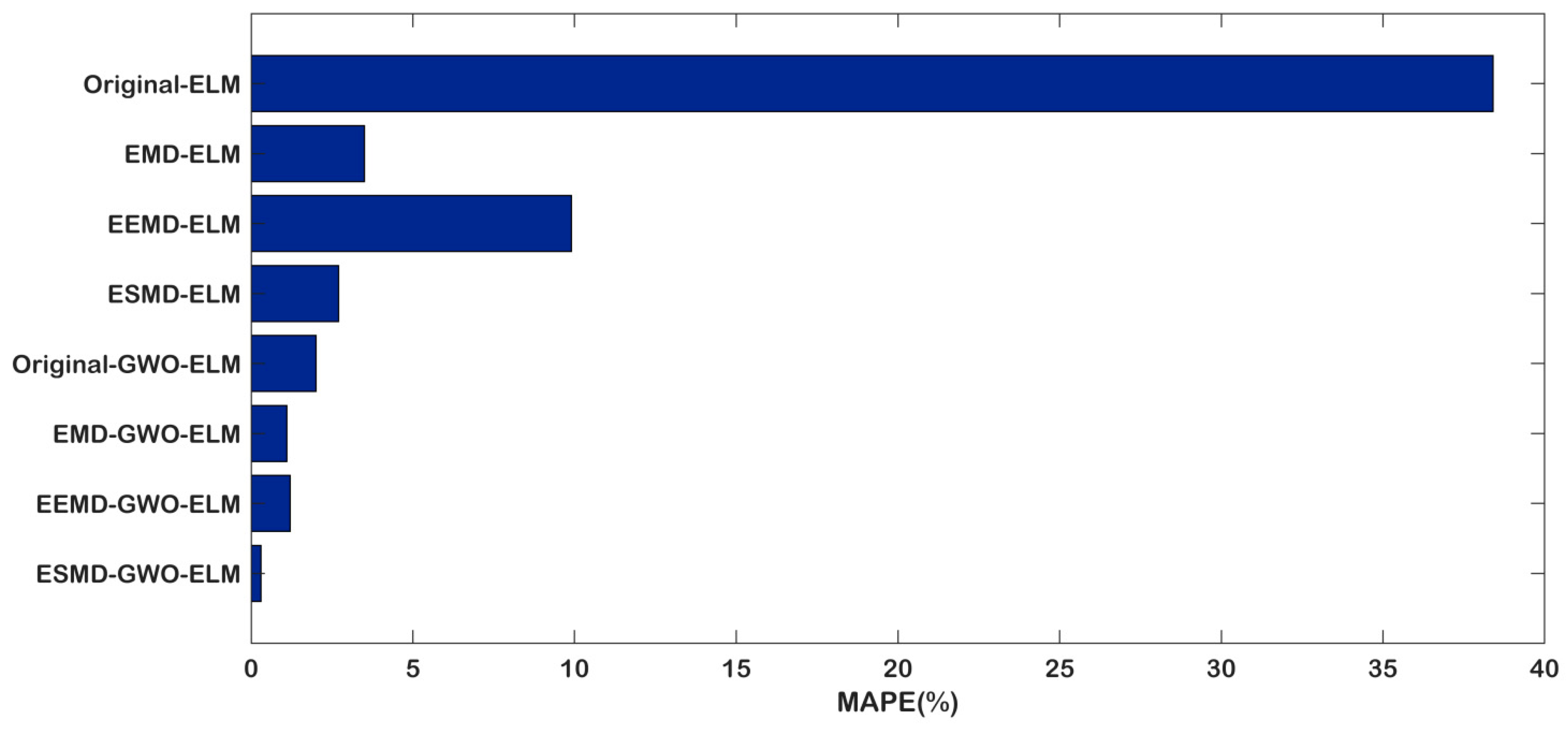
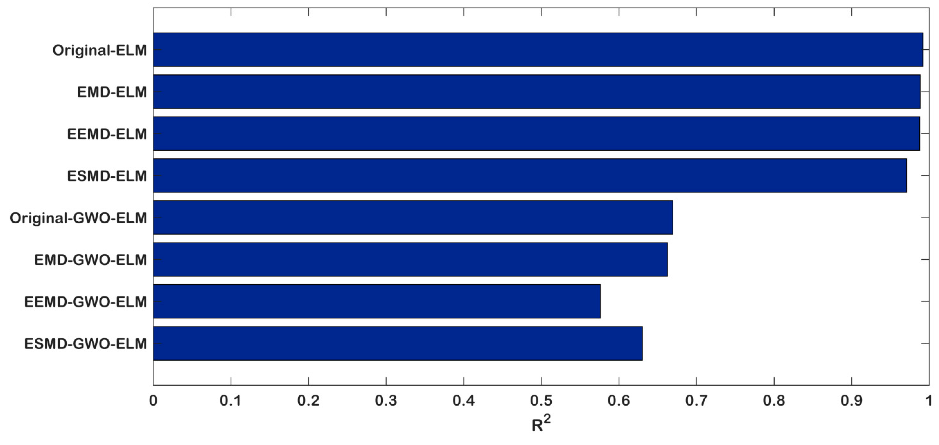
The proposed model ESMD-GWO-ELM has the lowest RMSE (0.1438) and MAPE (0.31), and highest R² (0.9918), which illustrates that the model performs significantly better than all of the considered benchmark models in the carbon price forecasting of Hubei.

(b)

Compared with the eight models, the Original-ELM model is the worst-performing, as it has the biggest RMSE (6.0734), MAPE (38.42), and lowest R² (0.6304). This is primarily due to the fact that the original carbon price is unstable and nonlinear, so that the single model is not fit for direct forecasting without decomposition processing.

(c)

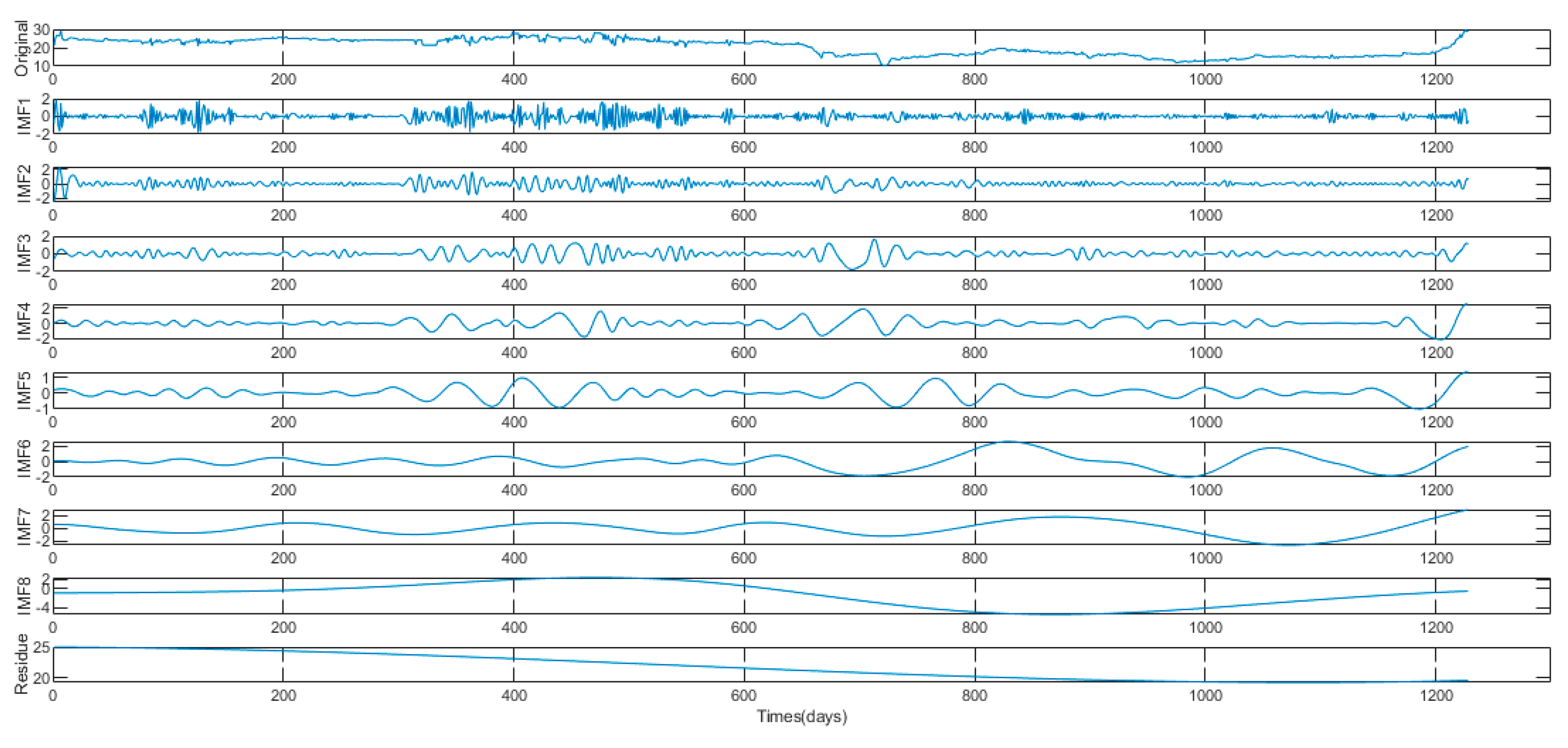
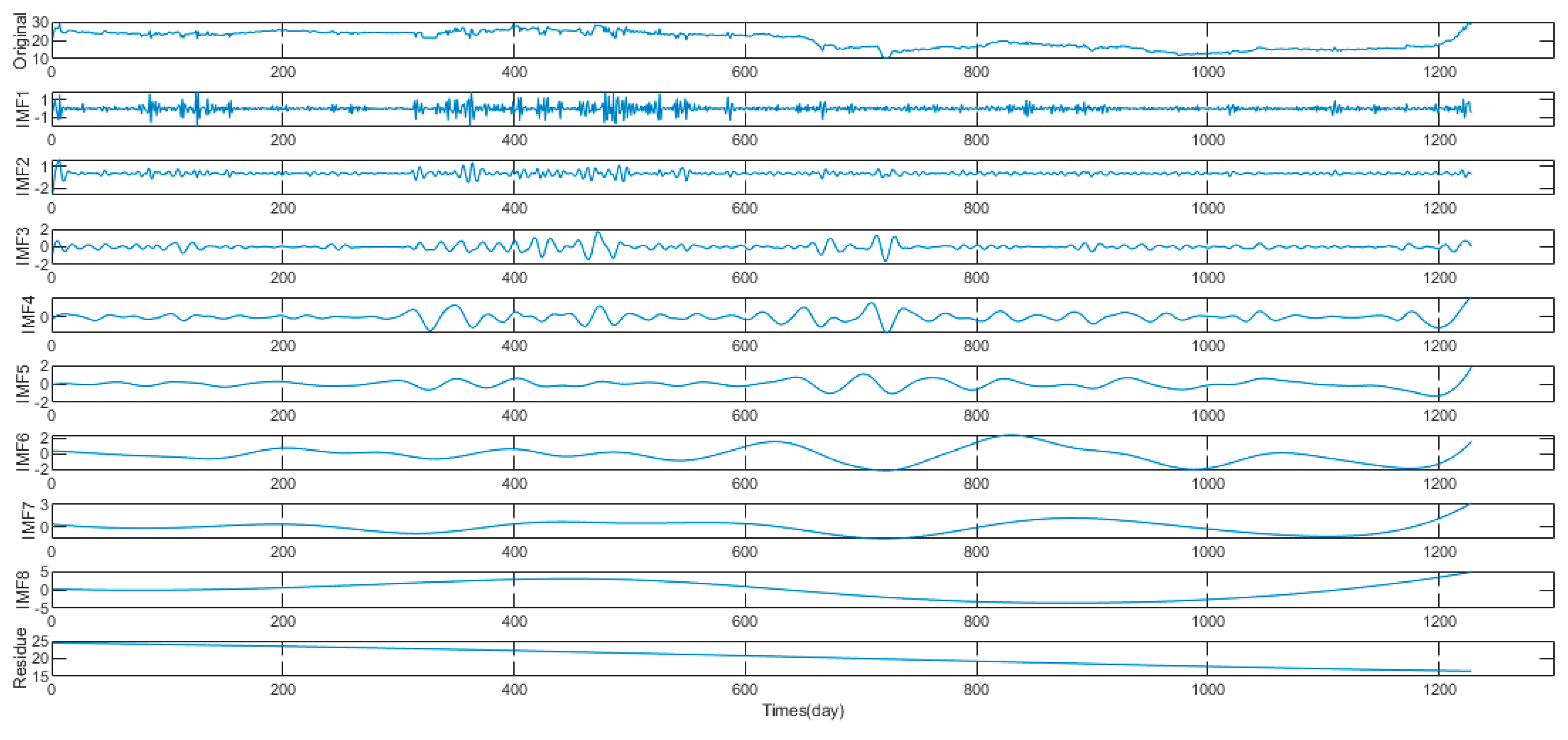
In the Original-ELM, EMD-ELM, EEMD-ELM, ESMD-ELM prediction models, the decomposed prediction models are obviously superior to the direct-prediction models. The main reason is that the structure and fluctuation of the decomposed IMF sequence become simpler and more stable, which enhances the forecast precision.

(d)

Compare with individual models (Original-ELM, EMD-ELM, EEMD-ELM, and ESMD-ELM) with optimized models (Original-GWO-ELM, EMD-GWO-ELM, EEMD-GWO-ELM, and ESMD-GWO-ELM), it is apparent that the GWO-ELM is significantly superior to the ELM model. This result demonstrates that the optimizing ELM parameter is necessary and meaningful.

(e)

It is evident that the ESMD decomposition method performs better than the EMD and EEMD methods, whatever the ESMD-ELM or ESMD-GWO-ELM, when compared to the decomposed models (EMD, EEMD, and ESMD). The result proves the superiority of the ESMD decomposition model.

(f)

However, compared with the EMD and EEMD methods, it is hard to decide which one is better. As shown in Table 7, the RMSE (1.7352) and MAPE (3.51) values of EMD-ELM are lower than those of EEMD-ELM (2.3936 and 9.92 respectively), which leads to the conclusion that the EMD-ELM performs better. However, when we compare the EMD-GWO-ELM and EEMD-GWO-ELM, the RMSE value of EEMD-GWO-ELM is 0.1917, which is lower than the value of 0.2559 of EMD-GWO-ELM; the R² value is higher, but the MAPE value is bigger than the EMD-GWO-ELM. Therefore, the EEMD decomposes the model performances better than the EMD. Above all, there is not enough evidence on which to judge which one is better. Thus, this conclusion will be demonstrated in the following section.

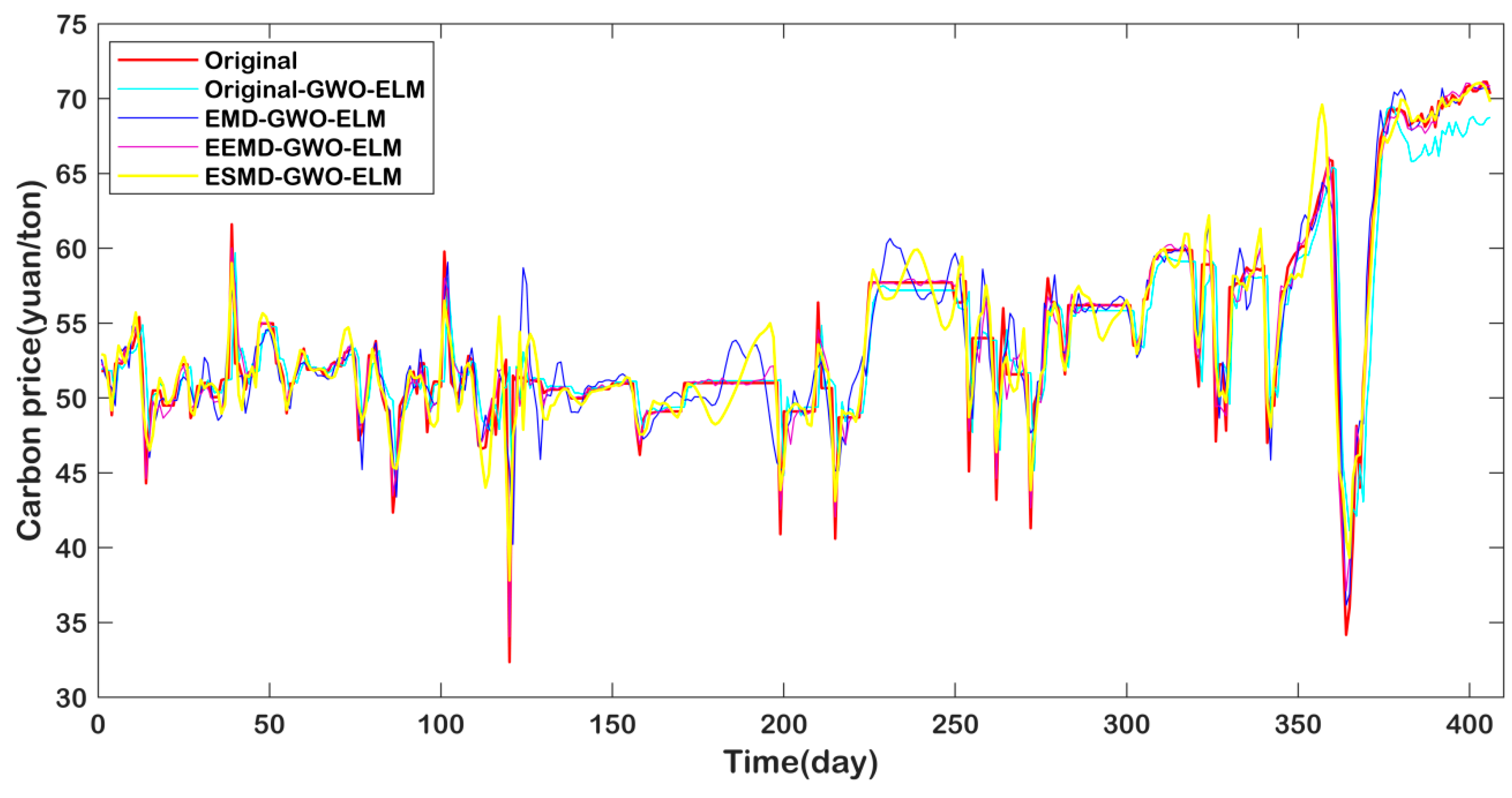
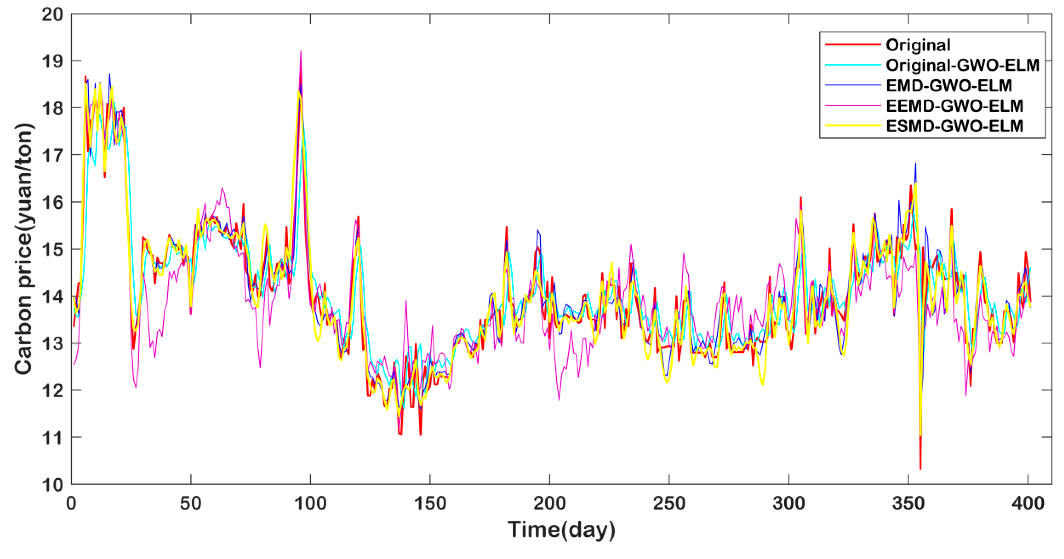
4.7. Additional Forecasting Case

In order to further prove the prediction accuracy of the proposed method, the carbon price series of Beijing, Guangdong, and Shanghai are predicted in this paper. Figure 15, Figure 16 and Figure 17 indicate the forecasting results. Also, the comparisons of the RMSE, MAPE, and R² between the models are shown in

Table 8. Analysis of the Beijing, Guangdong, and Shanghai forecasting results.

Model	Beijing			Guangdong			Shanghai
	RMSE	MAPE (%)	R2	RMSE	MAPE (%)	R2	RMSE	MAPE (%)	R2
Original-GWO-ELM	2.8518	0.16	0.7982	0.6847	0.67	0.7419	1.1340	0.03	0.9316
EMD-GWO-ELM	2.0934	0.34	0.8925	0.4168	0.35	0.9064	0.8362	0.10	0.9622
EEMD-GWO-ELM	1.8768	0.13	0.8957	0.6338	0.59	0.7875	0.7311	0.07	0.9700
ESMD-GWO-ELM	1.8069	0.03	0.9192	0.3835	0.11	0.9213	0.6948	0.05	0.9739

. As Table 8 shows, the RMSE and MAPE are the lowest, and the R² is the highest in the ESMD-GWO-ELM model between the models of the three markets, which further proved the prediction accuracy of the proposed model. Notice that the prediction accuracies of the EEMD-GWO-ELM model for Beijing and Shanghai are better than EMD-GWO-ELM. However, the forecasting performance of EMD-GWO-ELM is better than for EEMD-GWO-ELM in the Guangdong market. Consequently, it is hard to judge which one is better, for the reason that the results are not exactly matched. Nonetheless, it is evident that the ESMD-GWO-ELM model obtains the best prediction accuracies for the three markets. Both the RMSE and MAPE are the lowest, and the R² is the highest, between these models.

Undoubtedly, this study can draw the conclusion that the proposed model, the ESMD-GWO-ELM model, achieves the highest level of accuracy according to the results, which indicate that the proposed model is suitable for effective forecasting of the carbon price, when only considering historical carbon price series.

5. Conclusions

This paper proposes a new novel hybrid model for carbon price prediction, including extreme-point symmetric mode decomposition, extreme learning machine, and the grey wolf optimizer algorithm, which are applied to forecast the four carbon price series of China’s carbon trading pilot markets. Accordingly, three main steps are involved: firstly, owing to the nonlinear and non-stationary nature of carbon price, this study carried out decomposition models to decompose the carbon price into several IMFs and one residue. Then, the PACF is utilized to determine the input variables of each subsequence for the resulting forecasting models. Thirdly, this paper cultivates the GWO-ELM model to predict each decomposition component, and to add them. Moreover, the decomposition method and the prediction method constitute the comparative mixed model. The decomposition models include EMD, EEMD, and ESMD. Also, the prediction methods are ELM and GWO-ELM. To verify the practicability and effectiveness further, the carbon price series of Hubei, Beijing, Shanghai, and Guangdong are selected for the predictions. The results illustrate that the proposed model performs significantly better than all of the considered benchmark models. To conclude, the proposed model is suitable for forecasting the non-stationary and nonlinear carbon price. Several conclusions can be obtained from this paper: (a) The decomposed prediction models (EMD, EEMD, and ESMD) are obviously superior to the direct prediction models, based on the forecasting results, which indicates that it is necessary to decompose the non-stationary and nonlinear carbon price. (b) During the processing of carbon price forecasting, the models with ESMD perform better than those with EMD and EEMD. However, there is not enough evidence between the EMD and EEMD models to prove which one is better. (c) The proposed model, ESMD-GWO-ELM, performs better than the other methods for China carbon price prediction, when only the historical carbon price sequences are taken into account.

To conclude, this study provides a new approach for forecasting the carbon prices of China’s regional carbon emissions trading market. The conclusions obtained can provide guidance for carbon price predictions. In addition, this paper can obtain future carbon price changes for carbon trading markets, according to the above-described technical route in practical application, which is conductive to policy makers and inventors. Policy makers could adjust the price range of the price and the quantity of the market stability reserve, to guarantee the positive operation of the carbon trading market. Accordingly, the forecasting model could guide investors to obtain a clear understanding of the carbon trading market, and make reasonable investments.

References

1. Fan, J.H.; Todorova, N. Dynamics of China’s carbon prices in the pilot trading phase. Appl. Energy 2017, 208, 1452–1467. [Google Scholar] [CrossRef]
2. Dormady, N.C. Carbon auctions, energy markets & market power: An experimental analysis. Energy Econ. 2014, 44, 468–482. [Google Scholar]
3. Zhu, B.; Ye, S.; Wang, P.; He, K.; Zhang, T.; Wei, Y.-M. A novel multiscale nonlinear ensemble leaning paradigm for carbon price forecasting. Energy Econ. 2018, 70, 143–157. [Google Scholar] [CrossRef]
4. Zhu, J.; Wu, P.; Chen, H.; Liu, J.; Zhou, L. Carbon price forecasting with variational mode decomposition and optimal combined model. Phys. A-Stat. Mech. Its Appl. 2019, 519, 140–158. [Google Scholar] [CrossRef]
5. Karplus, V.J. Institutions and Emissions Trading in China. AEA Pap. Proc. 2018, 108, 468–472. [Google Scholar] [CrossRef]
6. Sun, W.; Zhang, C. Analysis and forecasting of the carbon price using multi—Resolution singular value decomposition and extreme learning machine optimized by adaptive whale optimization algorithm. Appl. Energy 2018, 231, 1354–1371. [Google Scholar] [CrossRef]
7. Yi, L.; Li, Z.-P.; Yang, L.; Liu, J.; Liu, Y.-R. Comprehensive evaluation on the “maturity” of China’s carbon markets. J. Clean. Prod. 2018, 198, 1336–1344. [Google Scholar] [CrossRef]
8. Tan, X.; Wang, X. The market performance of carbon trading in China: A theoretical framework of structure-conduct-performance. J. Clean. Prod. 2017, 159, 410–424. [Google Scholar] [CrossRef]
9. World Bank; Ecofys. State and Trends of Carbon Pricing 2018; The World Bank: Washington, DC, USA, 2018. [Google Scholar]
10. Stiglitz, J.; Stern, N.; Duan, M.; Edenhofer, O.; Giraud, G.; Heal, G.; La Rovere, E.L.; Morris, A.; Moyer, E.; Pangestu, M.; et al. Report of the High-Level Commission on Carbon Prices; Carbon Pricing Leadership Coalition: Washington, DC, USA, 2017. [Google Scholar]
11. Stefano, C.S. Kallbekken;Anton Orlov, How to win public support for a global carbon tax. Nature 2019, 565, 289. [Google Scholar]
12. Zhang, Y.J.; Wei, Y.M. An overview of current research on EU ETS: Evidence from its operating mechanism and economic effect. Appl. Energy 2010, 87, 1804–1814. [Google Scholar] [CrossRef]
13. Hepburn, C.; Neuhoff, K.; Acworth, W.; Burtraw, D.; Jotzo, F. The Economics of the EU ETS Market Stability Reserve. J. Environ. Econ. Manag. 2016, 80, 1–5. [Google Scholar] [CrossRef]
14. Keppler, J.H.; Mansanet-Bataller, M. Causalities between CO, electricity, and other energy variables during phase I and phase II of the EU ETS. Energy Policy 2010, 38, 3329–3341. [Google Scholar] [CrossRef]
15. Zeitlberger, A.C.M.; Brauneis, A. Modeling carbon spot and futures price returns with GARCH and Markov switching GARCH models. Cent. Eur. J. Oper. Res. 2014, 24, 1–28. [Google Scholar] [CrossRef]
16. Bredin, D.; Parsons, J.E. Why is Spot Carbon so Cheap and Future Carbon so Dear? The Term Structure of Carbon Prices. Energy J. 2016, 37. [Google Scholar] [CrossRef]
17. Zhu, B.; Chevallier, J.; Ma, S.; Wei, Y. Examining the structural changes of European carbon futures price 2005–2012. Appl. Econ. Lett. 2017, 22, 335–342. [Google Scholar] [CrossRef]
18. Arouri, M.E.H.; Jawadi, F.; Nguyen, D.K. Nonlinearities in carbon spot-futures price relationships during Phase II of the EU ETS. Econ. Model. 2012, 29, 884–892. [Google Scholar] [CrossRef]
19. Kanamura, T. Role of carbon swap trading and energy prices in price correlations and volatilities between carbon markets. Energy Econ. 2016, 54, 204–212. [Google Scholar] [CrossRef]
20. Chen, X.; Liu, M.; Liu, Y.; University, S.N. Price Drivers and Structural Breaks in China’s Carbon Prices:Based on Seven Carbon Trading Pilots. Econ. Probl. 2016, 11, 29–35. [Google Scholar]
21. Tan, X.-P.; Wang, X.-Y. Dependence changes between the carbon price and its fundamentals: A quantile regression approach. Appl. Energy 2017, 190, 306–325. [Google Scholar] [CrossRef]
22. Hammoudeh, S.; Nguyen, D.K.; Sousa, R.M. Energy prices and CO2 emission allowance prices: A quantile regression approach. Energy Policy 2014, 70, 201–206. [Google Scholar] [CrossRef]
23. Aatola, P.; Ollikainen, M.; Toppinen, A. Price determination in the EU ETS market: Theory and econometric analysis with market fundamentals. Energy Econ. 2013, 36, 380–395. [Google Scholar] [CrossRef]
24. Zhao, X.G.; Wu, L.; Li, A. Research on the efficiency of carbon trading market in China. Renew. Sustain. Energy Rev. 2017, 79, 1–8. [Google Scholar] [CrossRef]
25. Daskalakis, G. On the efficiency of the European carbon market: New evidence from Phase II. Energy Policy 2013, 54, 369–375. [Google Scholar] [CrossRef]
26. Montagnoli, A.; Vries, F.P.D. Carbon trading thickness and market efficiency. Energy Econ. 2010, 32, 1331–1336. [Google Scholar] [CrossRef] [Green Version]
27. Daskalakis, G.; Markellos, R.N. Are the European Carbon Markets Efficient? Soc. Sci. Electron. Publ. 2008, 17. [Google Scholar]
28. Zhang, J.; Li, D.; Hao, Y.; Tan, Z. A hybrid model using signal processing technology, econometric models and neural network for carbon spot price forecasting. J. Clean. Prod. 2018, 204, 958–964. [Google Scholar] [CrossRef]
29. Tsai, M.T.; Kuo, Y.T. Application of Radial Basis Function Neural Network for Carbon Price Forecasting. Appl. Mech. Mater. 2014, 590, 683–687. [Google Scholar] [CrossRef]
30. Guðbrandsdóttir, H.N.; Haraldsson, H.Ó. Predicting the Price of EU ETS Carbon Credits. Syst. Eng. Procedia 2011, 1, 481–489. [Google Scholar] [CrossRef] [Green Version]
31. Byun, S.J.; Cho, H. Forecasting carbon futures volatility using GARCH models with energy volatilities. Energy Econ. 2013, 40, 207–221. [Google Scholar] [CrossRef]
32. Glosten, L.R.; Jagannathan, R.; Runkle, D.E. On the Relation between the Expected Value and the Volatility of the Nominal Excess Return on Stocks. J. Financ. 1993, 48, 1779–1801. [Google Scholar] [CrossRef] [Green Version]
33. Chevallier, J. Volatility forecasting of carbon prices using factor models. Econ. Bull. 2010, 30, 1642–1660. [Google Scholar]
34. Chevallier, J. Nonparametric modeling of carbon prices. Energy Econ. 2011, 33, 1267–1282. [Google Scholar] [CrossRef]
35. Conrad, C.; Rittler, D.; Rotfuß, W. Modeling and explaining the dynamics of European Union Allowance prices at high-frequency. Energy Econ. 2010, 34, 316–326. [Google Scholar] [CrossRef]
36. Sanin, M.E.; Violante, F.; Mansanet-Bataller, M. Understanding volatility dynamics in the EU-ETS market. Energy Policy 2015, 82, 321–331. [Google Scholar] [CrossRef] [Green Version]
37. Koop, G.; Tole, L. Forecasting the European Carbon Market. J. R. Stat. Soc. 2013, 176, 723–741. [Google Scholar] [CrossRef]
38. Tsai, M.-T.; Kuo, Y.-T. A Forecasting System of Carbon Price in the Carbon Trading Markets Using Artificial Neural Network. Int. J. Environ. Sci. Dev. 2013, 4, 163–167. [Google Scholar] [CrossRef]
39. Zhu, B.; Chevallier, J. Carbon Price Forecasting with a Hybrid ARIMA and Least Squares Support Vector Machines Methodology. Omega-Int. J. Manag. Sci. 2013, 41, 517–524. [Google Scholar] [CrossRef]
40. Atsalakis, G.S. Using computational intelligence to forecast carbon prices. Appl. Soft Comput. 2016, 43, 107–116. [Google Scholar] [CrossRef]
41. Fan, X.; Li, S.; Tian, L. Chaotic characteristic identification for carbon price and an multi-layer perceptron network prediction model. Expert Syst. Appl. 2015, 42, 3945–3952. [Google Scholar] [CrossRef]
42. Zhu, B. A Novel Multiscale Ensemble Carbon Price Prediction Model Integrating Empirical Mode Decomposition, Genetic Algorithm and Artificial Neural Network. Energies 2012, 5, 355–370. [Google Scholar] [CrossRef] [Green Version]
43. Sun, G.; Chen, T.; Wei, Z.; Sun, Y.; Zang, H.; Chen, S. A Carbon Price Forecasting Model Based on Variational Mode Decomposition and Spiking Neural Networks. Energies 2016, 9, 54. [Google Scholar] [CrossRef]
44. Zhu, B.; Chevallier, J. Forecasting Carbon Price with Empirical Mode Decomposition and Least Squares Support Vector Regression. Appl. Energy 2017, 191, 521–530. [Google Scholar] [CrossRef]
45. Feng, Z.-H.; Liu, C.-F.; Wei, Y.-M. How does carbon price change? Evidences from EU ETS. Int. J. Glob. Energy Issues 2011, 35, 132–144. [Google Scholar] [CrossRef]
46. Li, S.; Wang, P.; Goel, L. Short-term load forecasting by wavelet transform and evolutionary extreme learning machine. Electr. Power Syst. Res. 2015, 122, 96–103. [Google Scholar] [CrossRef]
47. Li, S.; Goel, L.; Wang, P. An ensemble approach for short-term load forecasting by extreme learning machine. Appl. Energy 2016, 170, 22–29. [Google Scholar] [CrossRef]
48. Shrivastava, N.A.; Panigrahi, B.K. A hybrid wavelet-ELM based short term price forecasting for electricity markets. Int. J. Electr. Power Energy Syst. 2014, 55, 41–50. [Google Scholar] [CrossRef]
49. Hui, L.; Mi, X.; Li, Y. An Experimental Investigation of Three New Hybrid Wind Speed Forecasting Models Using Multi-decomposing Strategy and ELM Algorithm. Renew. Energy 2018, 123, 694–705. [Google Scholar]
50. Abdoos, A.A. A new intelligent method based on combination of VMD and ELM for short term wind power forecasting. Neurocomputing 2016, 203, 111–120. [Google Scholar] [CrossRef]
51. Rocha, H.R.O.; Silvestre, L.J.; Celeste, W.C.; Coura, D.J.C.; Rigo, L.O., Jr. Forecast of Distributed Electrical Generation System Capacity Based on Seasonal Micro Generators using ELM and PSO. IEEE Lat. Am. Trans. 2018, 16, 1136–1141. [Google Scholar] [CrossRef]
52. Sun, W.M. Duan, Analysis and Forecasting of the Carbon Price in China’s Regional Carbon Markets Based on Fast Ensemble Empirical Mode Decomposition, Phase Space Reconstruction, and an Improved Extreme Learning Machine. Energies 2019, 12, 277. [Google Scholar] [CrossRef]
53. Wang, J.-L.; Li, Z.-J. Extreme-point symmetric mode decomposition method for data analysis. Adv. Adapt. Data Anal. 2013, 5, 1350015. [Google Scholar] [CrossRef]
54. Huang, G.B.; Zhu, Q.Y.; Siew, C.K. Extreme learning machine: A new learning scheme of feedforward neural networks. In Proceedings of the 2004 IEEE International Joint Conference on Neural Networks, Budapest, Hungary, 25–29 July 2004; Volume 2, pp. 985–990. [Google Scholar]
55. Huang, G.B.; Zhu, Q.Y.; Siew, C.K. Extreme learning machine: Theory and applications. Neurocomputing 2006, 70, 489–501. [Google Scholar] [CrossRef] [Green Version]
56. Mirjalili, S.; Mirjalili, S.M.; Lewis, A. Grey Wolf Optimizer. Adv. Eng. Softw. 2014, 69, 46–61. [Google Scholar] [CrossRef]
57. Shanmugam, R. Introduction to Time Series and Forecasting. Technometrics 1997, 39, 426. [Google Scholar] [CrossRef]
58. Qi, S.; Wang, B.; Zhang, J. Policy design of the Hubei ETS pilot in China. Energy Policy 2014, 75, 31–38. [Google Scholar] [CrossRef]
59. Lan, Y.; Zhaopeng, L.; Li, Y.; Jie, L. Comparative study on the development degree of China’s 7 pilot carbon markets. China Popul. Resour. Environ. 2018, 2, 134–140. [Google Scholar]
60. Liu, Y.; Tan, X.-J.; Yu, Y.; Qi, S.-Z. Assessment of impacts of Hubei Pilot emission trading schemes in China—A CGE-analysis using Term CO2 model. Appl. Energy 2017, 189, 762–769. [Google Scholar] [CrossRef]
61. Hu, Y.J.; Li, X.Y.; Tang, B.J. Assessing the operational performance and maturity of the carbon trading pilot program: The case study of Beijing’s carbon market. J. Clean. Prod. 2017, 161, 1263–1274. [Google Scholar] [CrossRef]
62. Available online: http://www.tanjiaoyi.com/ (accessed on 28 December 2018).
63. Dégerine, S.; Lambert-Lacroix, S. Characterization of the partial autocorrelation function of nonstationary time series. J. Multivar. Anal. 2003, 87, 46–59. [Google Scholar] [CrossRef] [Green Version]
64. Guo, Z.; Zhao, W.; Lu, H.; Wang, J. Multi-step forecasting for wind speed using a modified EMD-based artificial neural network model. Renew. Energy 2012, 37, 241–249. [Google Scholar] [CrossRef]
Figure 1. The hierarchy of grey wolves.
Energies 12 00950 g001
Figure 2. The process of the proposed GWO-ELM model.
Energies 12 00950 g002
Figure 3. The forecasting process for carbon price with ESMD-GWO-ELM model.
Energies 12 00950 g003
Figure 4. The carbon price fluctuations.
Energies 12 00950 g004
Figure 5. The results of the Hubei carbon price decomposed by ESMD.
Energies 12 00950 g005
Figure 6. The results of the Hubei carbon price decomposed by EMD.
Energies 12 00950 g006
Figure 7. The results of the Hubei carbon price, decomposed by EEMD.
Energies 12 00950 g007
Figure 8. The PCAF results of the Hubei carbon price after ESMD.
Energies 12 00950 g008
Figure 9. The PCAF results of the Hubei carbon price after EMD.
Energies 12 00950 g009
Figure 10. The PCAF results of the Hubei carbon price after EEMD.
Energies 12 00950 g010
Figure 11. The results of Hubei carbon price forecasting.
Energies 12 00950 g011
Figure 12. The values of the RMSE-parallel models.
Energies 12 00950 g012
Figure 13. The values of the MAPE parallel models.
Energies 12 00950 g013
Figure 14. The values of the R2 parallel models.
Energies 12 00950 g014
Figure 15. The results of Beijing carbon price forecasting.
Energies 12 00950 g015
Figure 16. The results of Guangdong carbon price forecasting.
Energies 12 00950 g016
Figure 17. The results of Shanghai carbon price forecasting.
Energies 12 00950 g017