An Optimum Enthalpy Approach for Melting and Solidification with Volume Change

Abstract
:1. Introduction
2. Mathematical Model
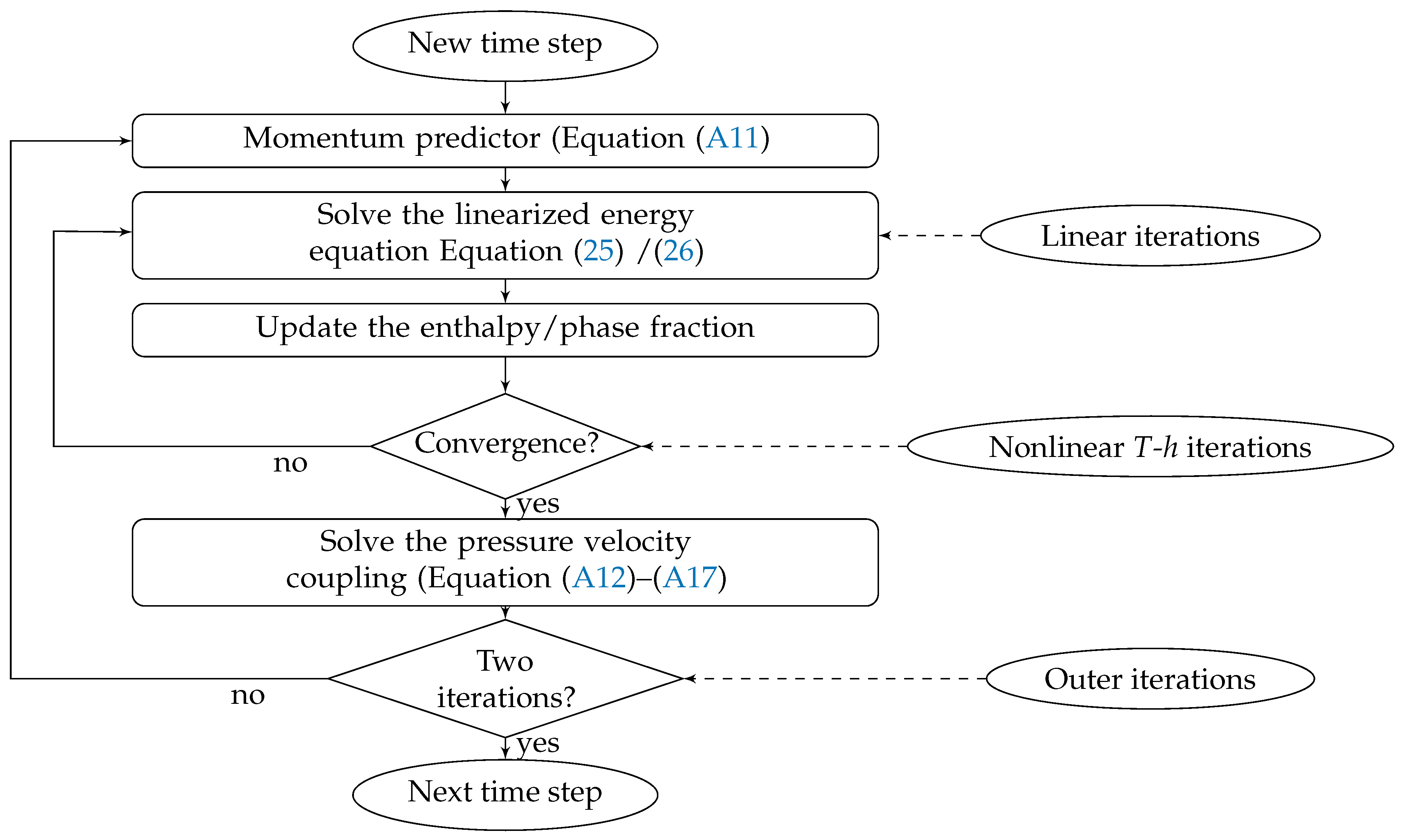
3. Numerical Solution
3.1. Optimum Approach
3.2. Optimum Density Approach
3.3. Source Based Method
3.4. Test Cases
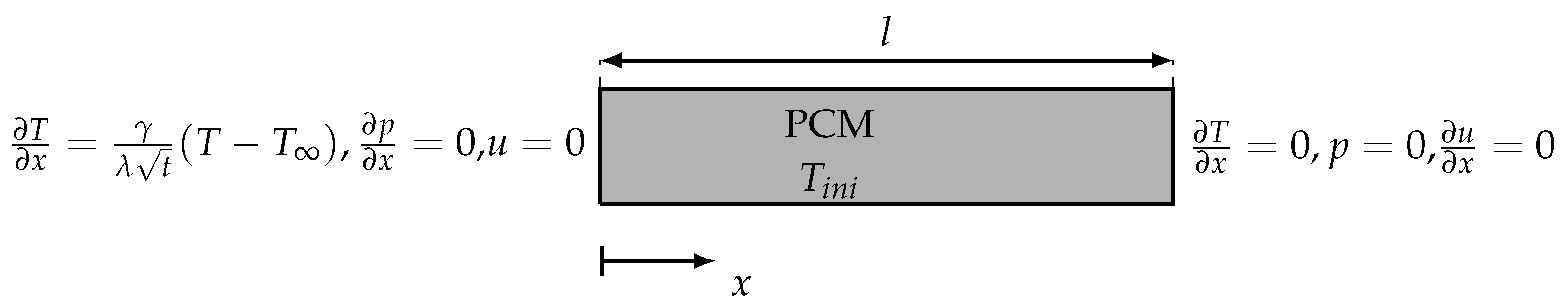
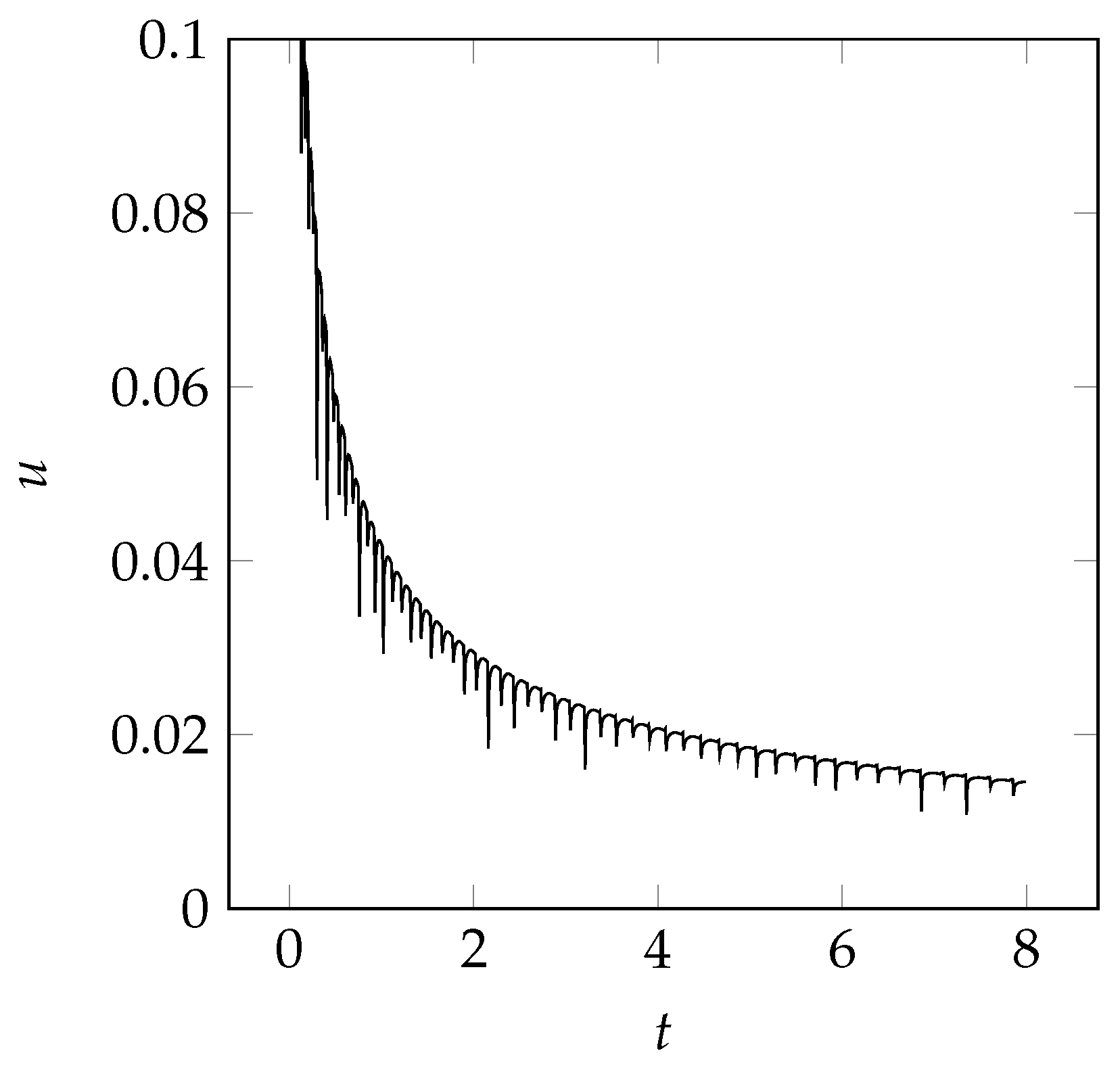
3.4.1. One-Dimensional Solidification
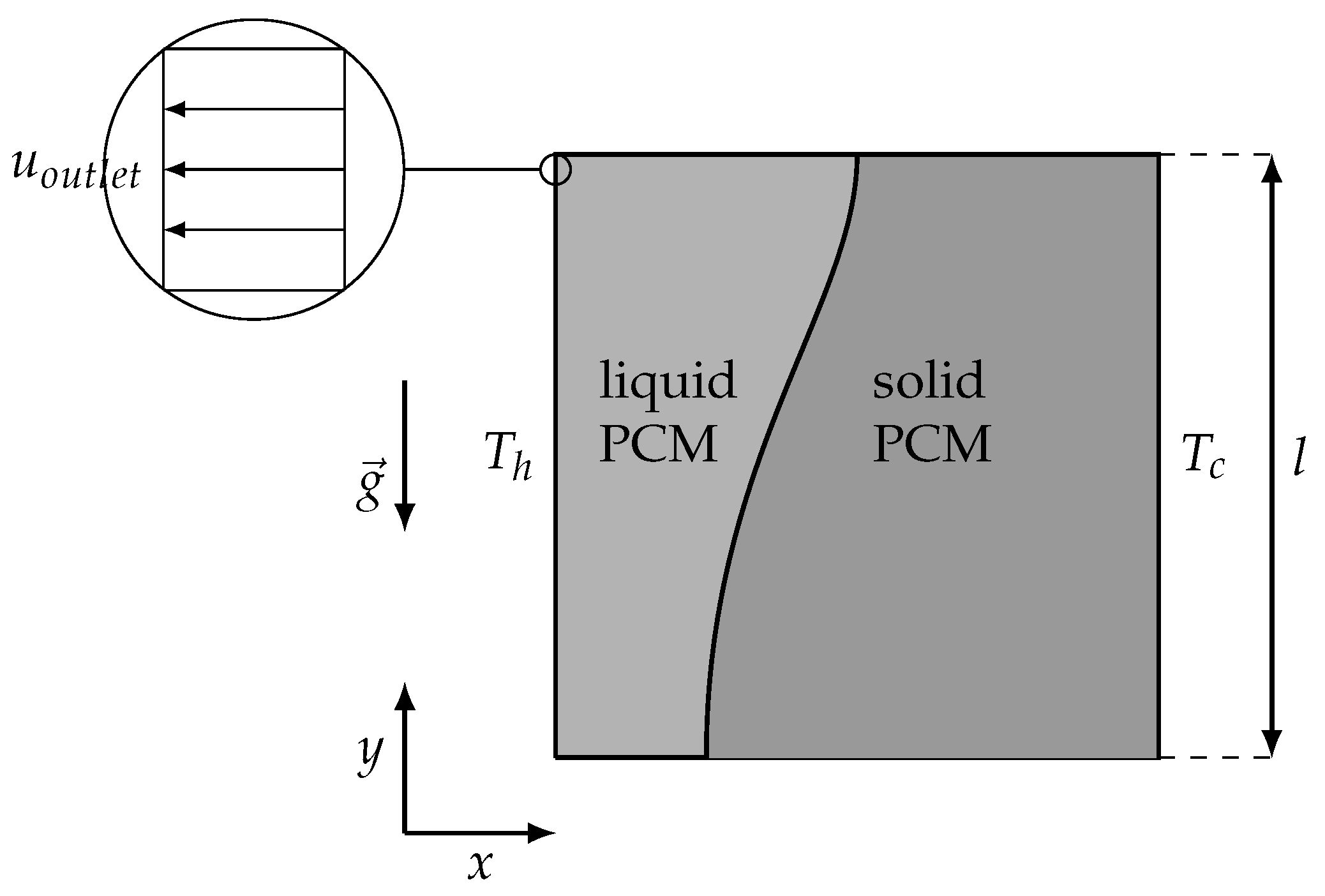
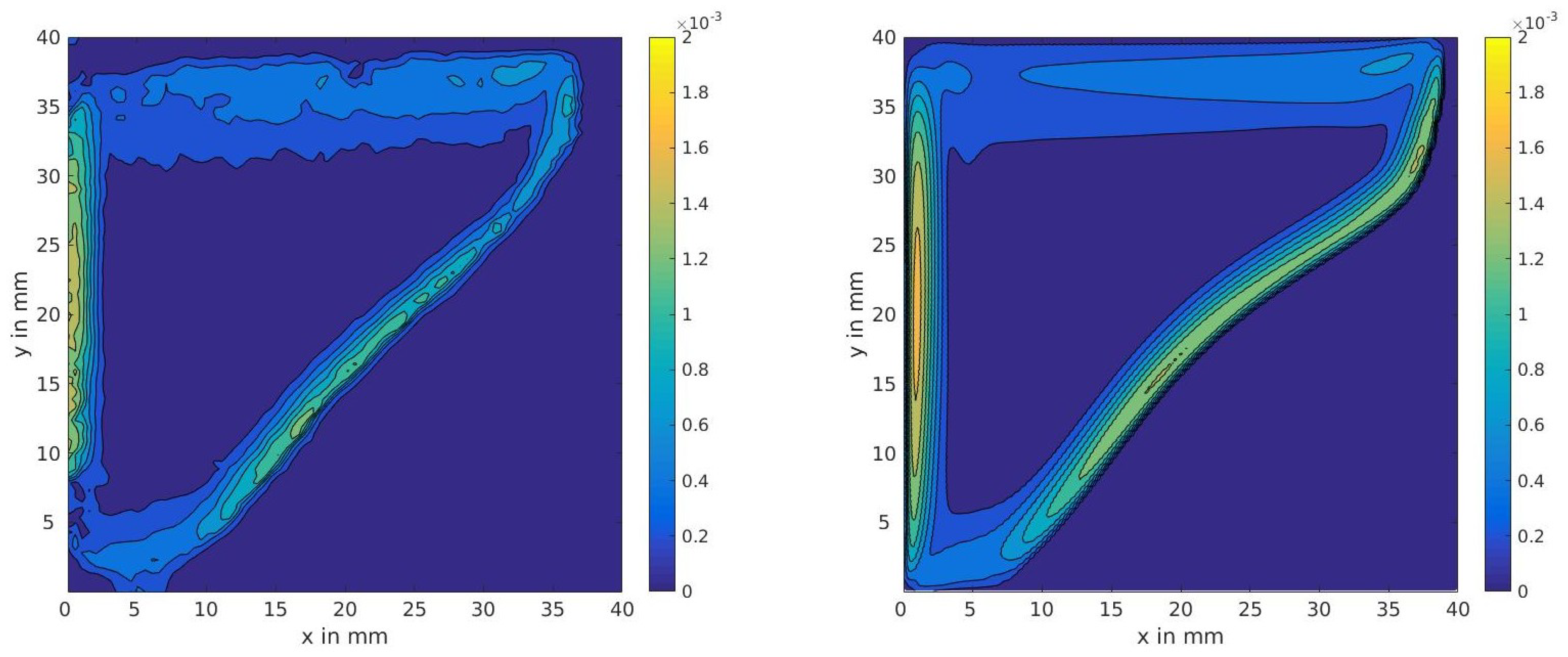
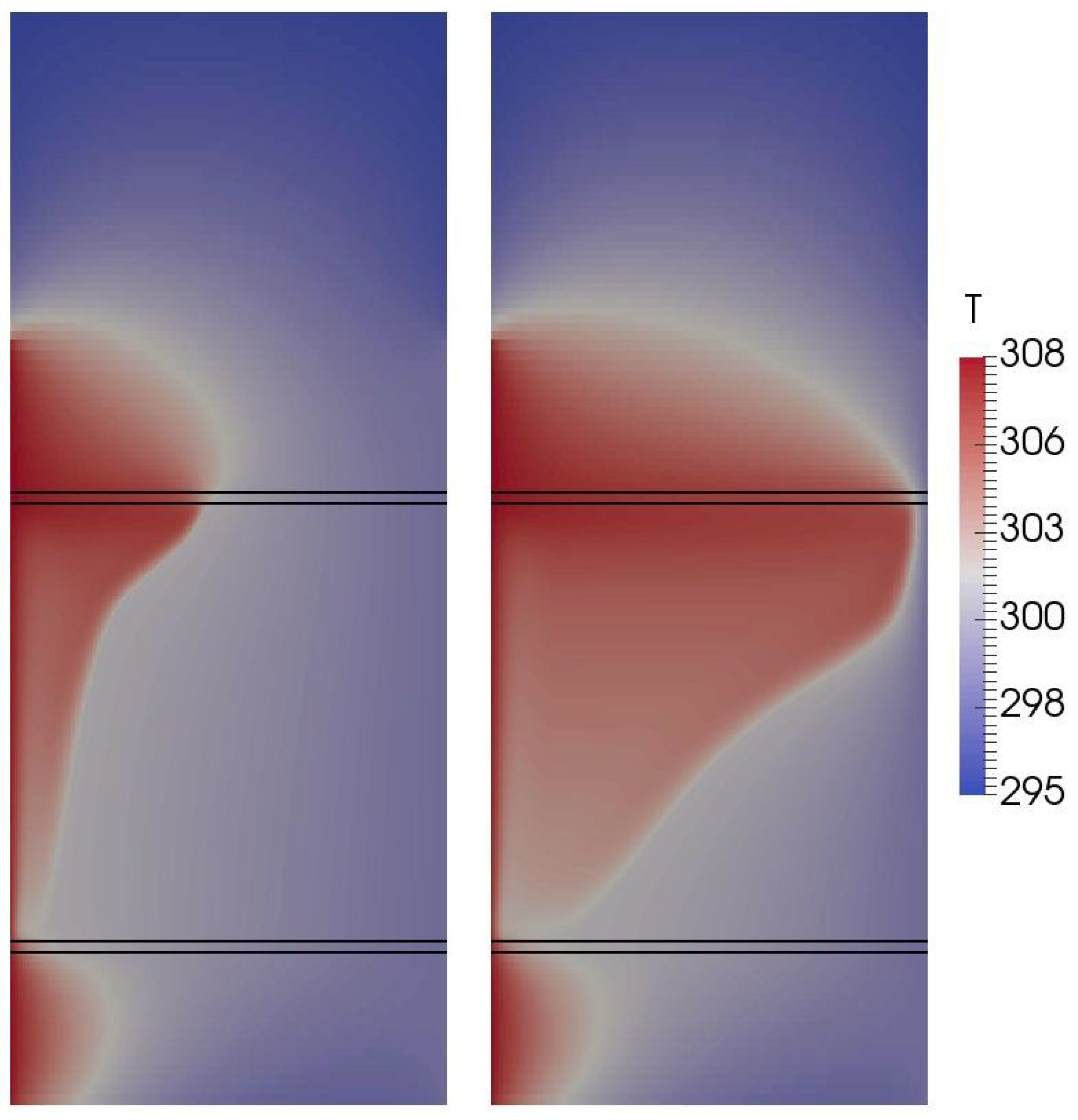
3.4.2. Two-Dimensional Melting with Convection
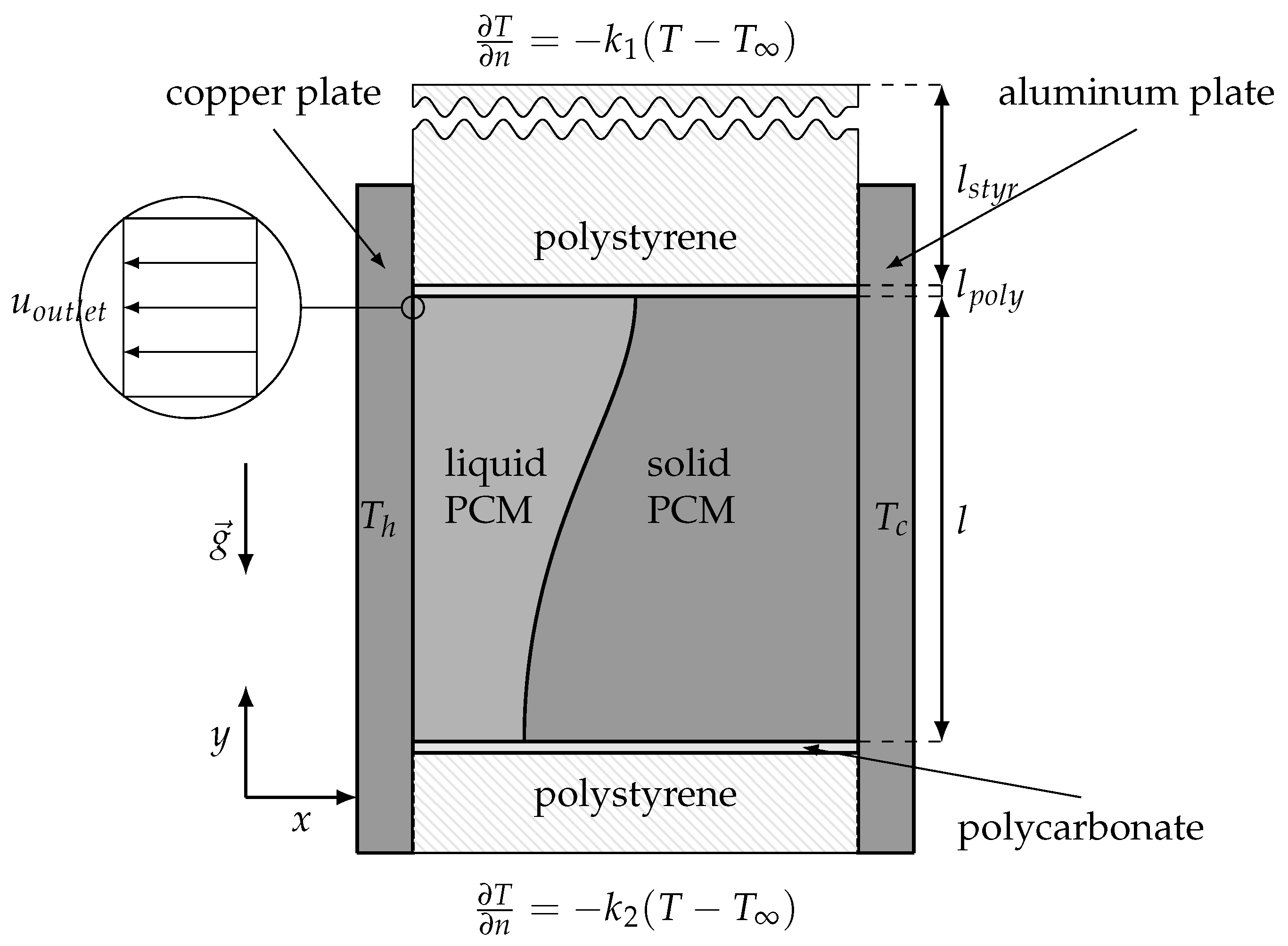
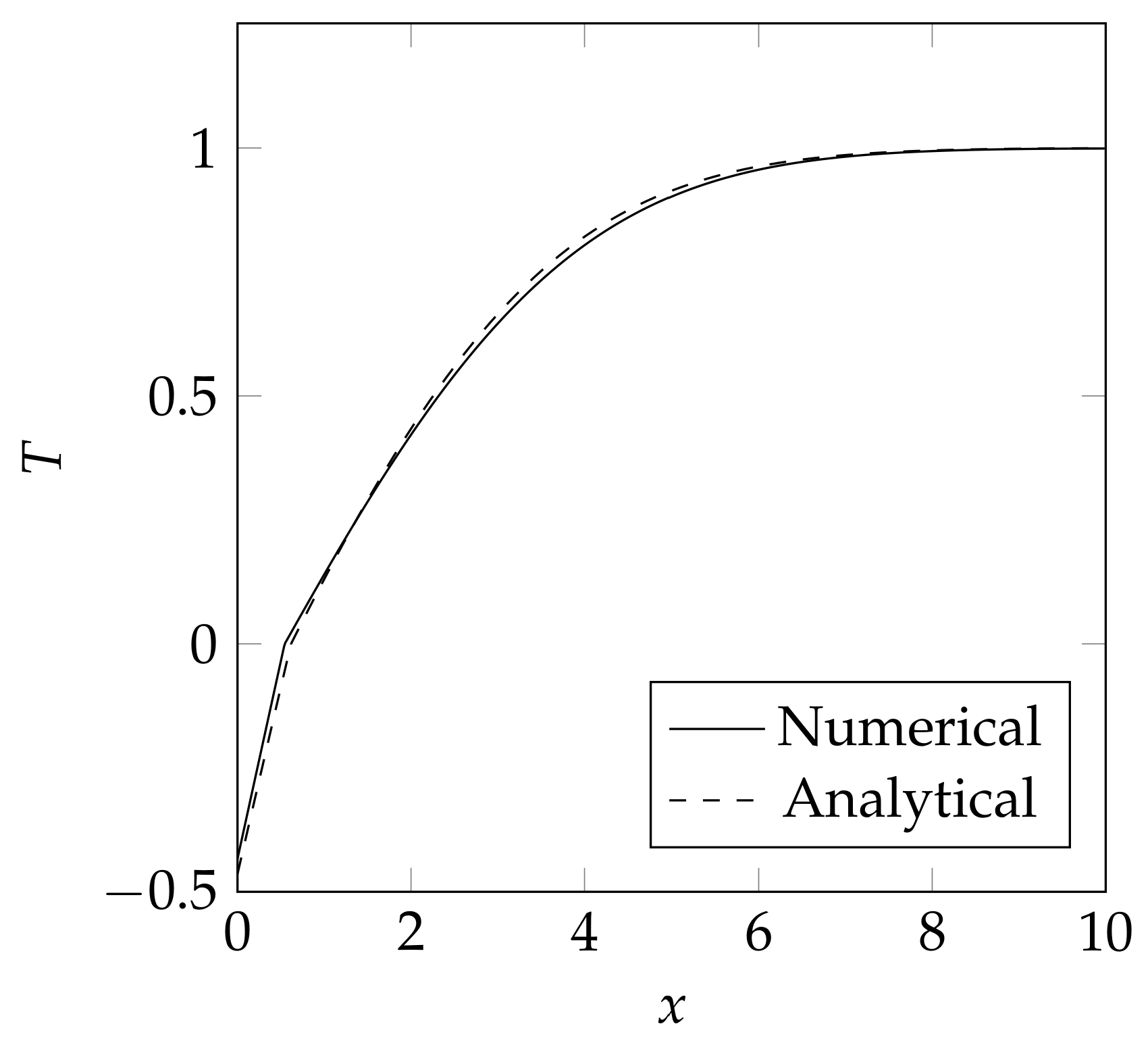
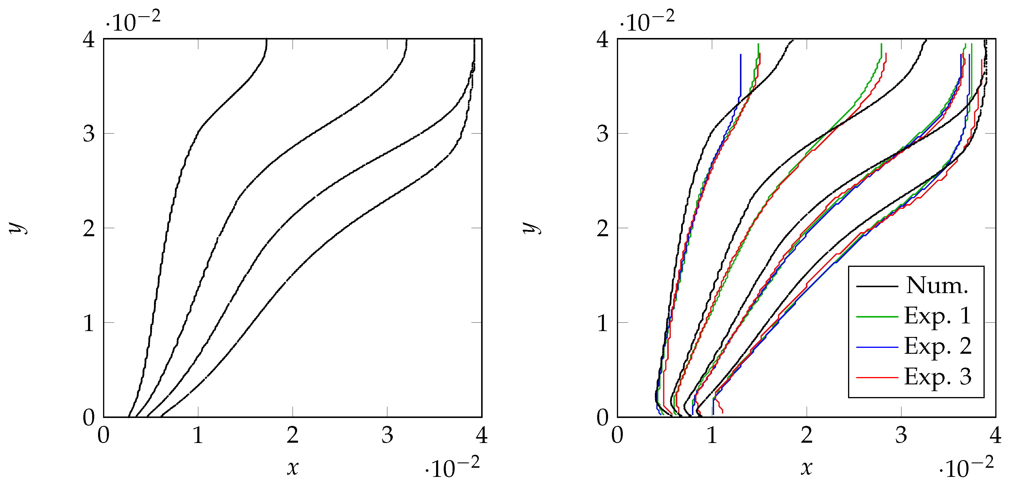
3.5. Validation Case
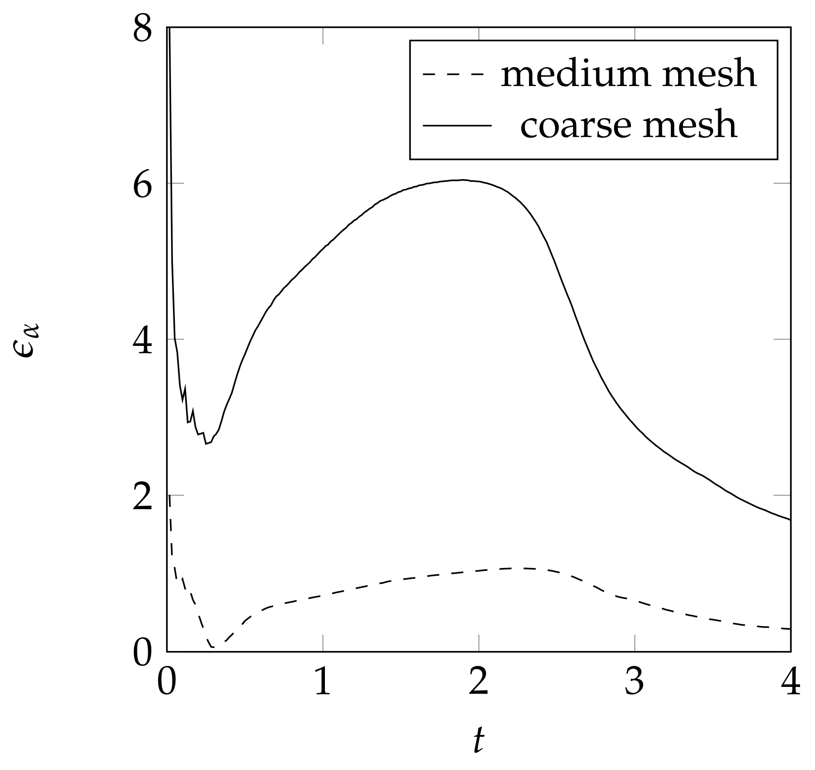
3.6. Mesh Influence for the Convection Test Case
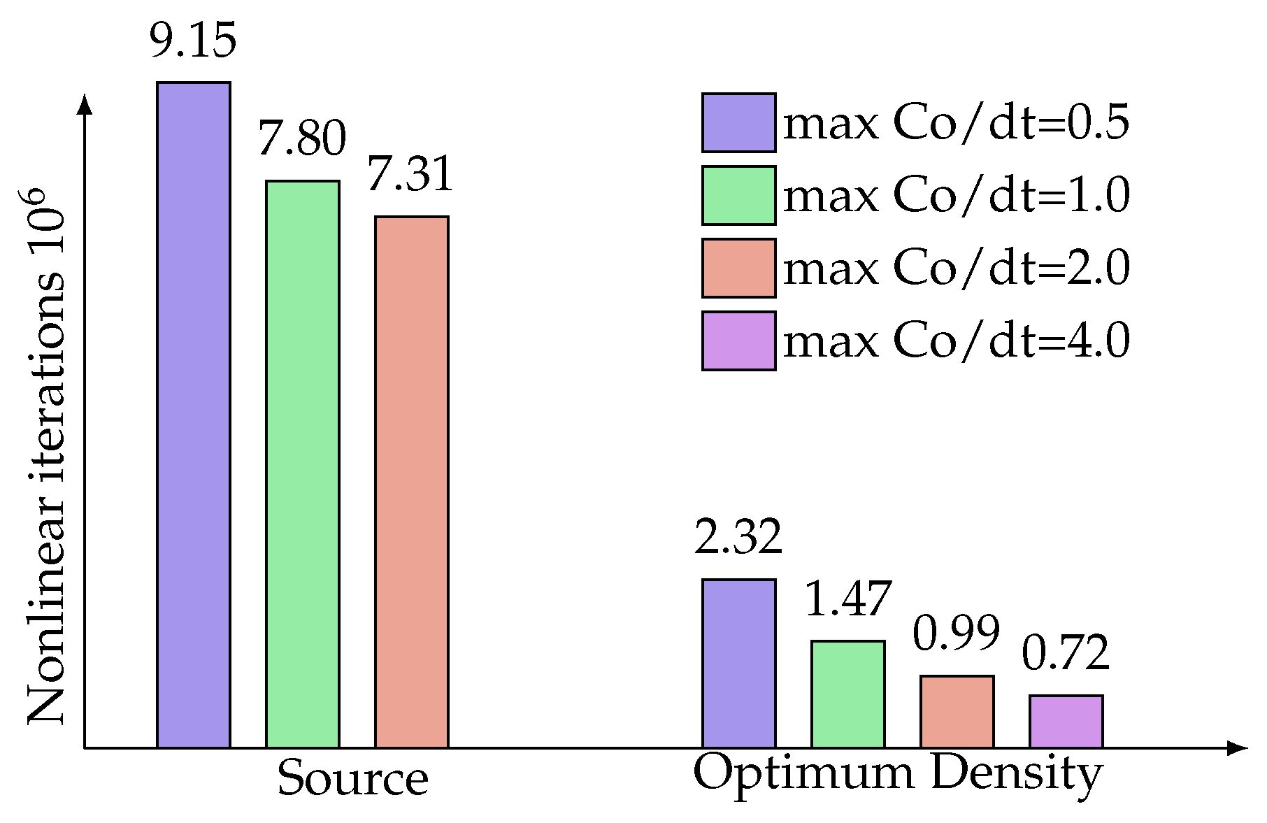
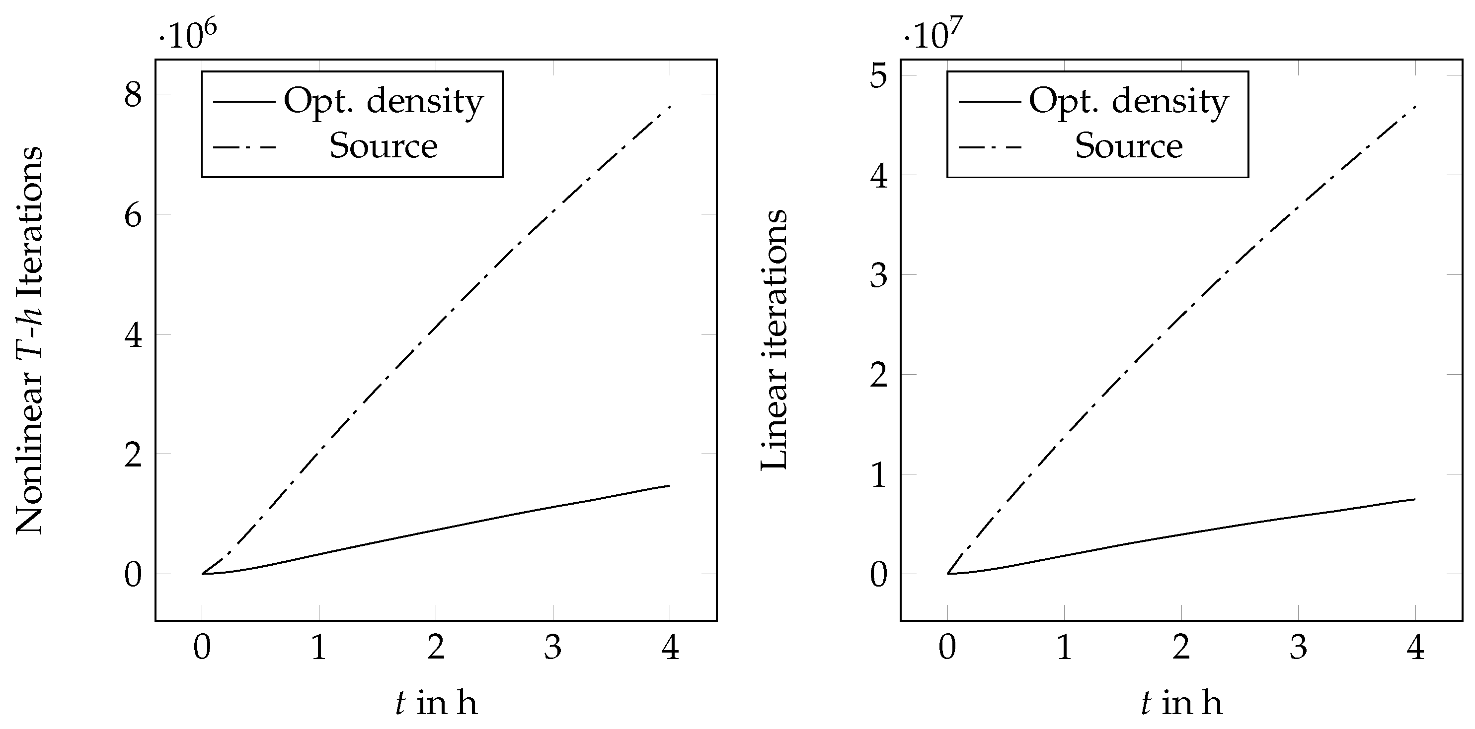
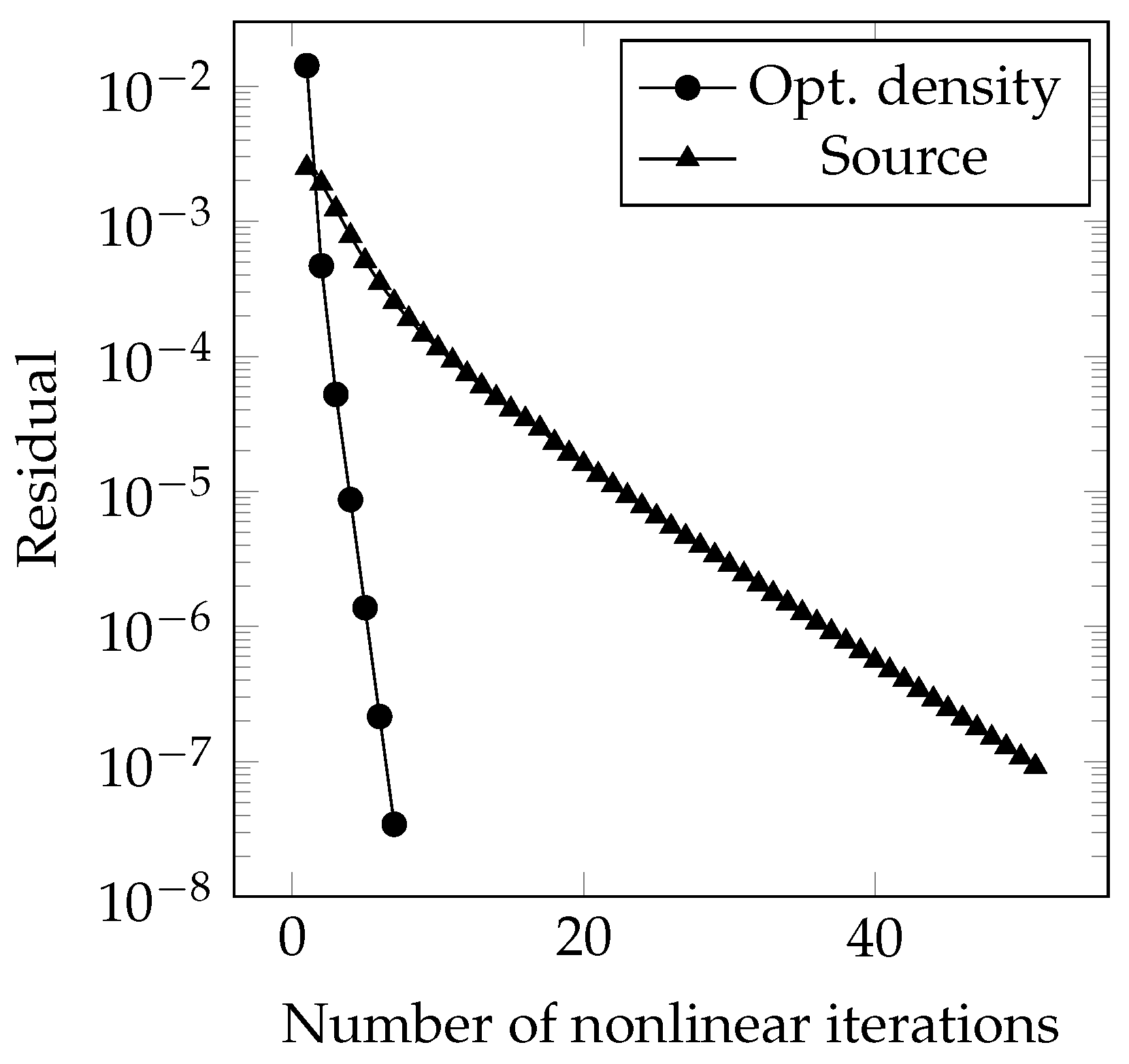
4. Results and Discussion
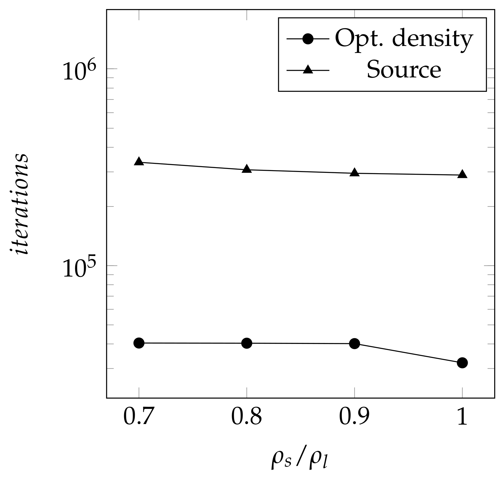
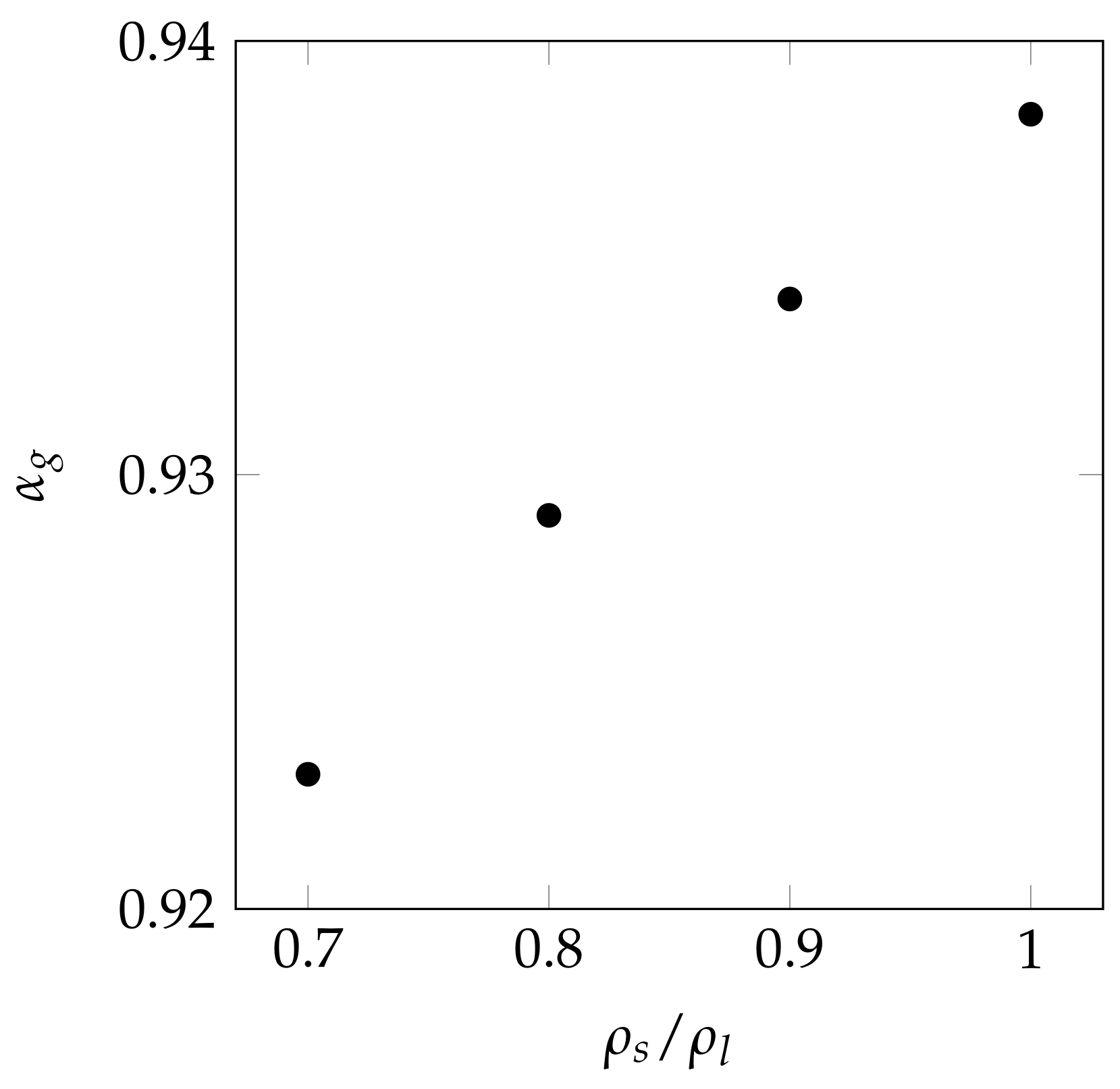
4.1. One-Dimensional Solidification
4.2. Two-Dimensional Melting of Octadecane with Natural Convection
4.3. Validation
5. Conclusions
Author Contributions
Funding
Conflicts of Interest
Nomenclature
| heat capacity | |
| f | function |
| h | enthalpy |
| gravitational acceleration | |
| k | heat transfer coefficient |
| l | length |
| m | mass |
| normalized gradient | |
| p | pressure |
| t | time |
| velocity vector | |
| x | coordinate |
| y | coordinate |
| Darcy term | |
| A | area |
| D | Darcy constant |
| E | identity matrix |
| L | latent heat of fusion |
| T | temperature |
| V | volume |
| phase fraction | |
| volumetric coefficient of thermal expansion | |
| abbreviation | |
| small numerical constant | |
| thermal conductivity | |
| viscosity | |
| density | |
| stress tensor | |
| underrelaxation factor | |
| c | cold |
| g | global |
| h | hot |
| i | index |
| initial | |
| k | index |
| l | liquid |
| m | index |
| o | old |
| reference | |
| residuum | |
| s | solid |
| y | y component |
| L | liquidus |
| S | solidus |
| T | transpose |
Appendix A
Appendix A.1. Derivation of the Pressure Equation
Appendix A.2. PISO-Algorithm
References
- Kuboth, S.; König-Haagen, A.; Brüggemann, D. Numerical analysis of shell-and-tube type latent thermal energy storage performance with different arrangements of circular fins. Energies 2017, 10, 274. [Google Scholar] [CrossRef]
- Kozak, Y.; Rozenfeld, T.; Ziskind, G. Close-contact melting in vertical annular enclosures with a non-isothermal base: Theoretical modeling and application to thermal storage. Int. J. Heat Mass Transf. 2014, 72, 114–127. [Google Scholar] [CrossRef]
- Brent, A.D.; Voller, V.R.; Reid, K.J. Enthalpy-Porosity Technique for Modeling Convection-Diffusion Phase Change: Application To the Melting of a Pure Metal. Numer. Heat Transf. 1988, 13, 297–318. [Google Scholar] [CrossRef]
- Voller, V.R. An overview of numerical methods for solving phase change problems. Adv. Numer. Heat Transf. 1996, 1, 341–380. [Google Scholar]
- Crank, J. Free and Moving Boundary Problems; Oxford Science Publications: New York, NY, USA, 1984. [Google Scholar]
- König-Haagen, A.; Franquet, E.; Pernot, E.; Brüggemann, D. A comprehensive benchmark of fixed-grid methods for the modeling of melting. Int. J. Therm. Sci. 2017, 118, 69–103. [Google Scholar] [CrossRef]
- Faden, M.; König-Haagen, A.; Höhlein, S.; Brüggemann, D. An implicit algorithm for melting and settling of phase change material inside macrocapsules. Int. J. Heat Mass Transf. 2018, 117, 757–767. [Google Scholar] [CrossRef]
- Rose, M.E. A Method for Calculating Solutions of Parabolic Equations with a Free Boundary. Math. Comput. 1960, 14, 249–256. [Google Scholar] [CrossRef]
- Solomon, A.D. Some Remarks on the Stefan Problem. Math. Comput. 1966, 20, 347–360. [Google Scholar] [CrossRef]
- Morgan, K. A numerical analysis of freezing and melting with convection. Comput. Methods Appl. Mech. Eng. 1981, 28, 275–284. [Google Scholar] [CrossRef]
- Gartling, D.K. Finite element analysis of convective heat transfer problems with change of phase. Comput. Methods Fluids 1980, 257–284. [Google Scholar]
- Voller, V.R.; Prakash, C. A fixed grid numerical modelling methodology for convection-diffusion mushy region phase-change problems. Int. J. Heat Mass Transf. 1987, 30, 1709–1719. [Google Scholar] [CrossRef]
- Swaminathan, C.R.; Voller, V.R. A general enthalpy method for modeling solidification processes. Metall. Trans. B 1992, 23, 651–664. [Google Scholar] [CrossRef]
- Swaminathan, C.R.; Voller, V.R. On the enthalpy method. Int. J. Numer. Methods Heat Fluid Flow 1993, 3, 233–244. [Google Scholar] [CrossRef]
- Danaila, I.; Moglan, R.; Hecht, F.; Le Masson, S. A Newton method with adaptive finite elements for solving phase-change problems with natural convection. J. Comput. Phys. 2014, 274, 826–840. [Google Scholar] [CrossRef]
- Assis, E.; Katsman, L.; Ziskind, G.; Letan, R. Numerical and experimental study of melting in a spherical shell. Int. J. Heat Mass Transf. 2007, 50, 1790–1804. [Google Scholar] [CrossRef]
- Assis, E.; Ziskind, G.; Letan, R. Numerical and Experimental Study of Solidification in a Spherical Shell. J. Heat Transf. 2009, 131, 24502–24506. [Google Scholar] [CrossRef]
- Galione, P.A.; Lehmkuhl, O.; Rigola, J.; Oliva, A. Fixed-grid numerical modeling of melting and solidification using variable thermo-physical properties - Application to the melting of n-Octadecane inside a spherical capsule. Int. J. Heat Mass Transf. 2015, 86, 721–743. [Google Scholar] [CrossRef]
- Hassab, M.A.; Sorour, M.M.; Khamis Mansour, M.; Zaytoun, M.M. Effect of volume expansion on the melting process’s thermal behavior. Appl. Therm. Eng. 2017, 115, 350–362. [Google Scholar] [CrossRef]
- Dallaire, J.; Gosselin, L. Numerical modeling of solid-liquid phase change in a closed 2D cavity with density change, elastic wall and natural convection. Int. J. Heat Mass Transf. 2017, 114, 903–914. [Google Scholar] [CrossRef]
- Faden, M.; Linhardt, C.; Höhlein, S.; König-Haagen, A.; Brüggemann, D. Velocity field and phase boundary measurements during melting of n-octadecane in a cubical test cell. Int. J. Heat Mass Transf. 2019, 135, 104–114. [Google Scholar] [CrossRef]
- Alexiades, V.; Drake, J.B. A weak formulation for phase-change problems with bulk movement due to unequal densities. In Free Boundary Problems Involving Solids; Longman: Harlow, UK, 1993; pp. 82–87. [Google Scholar]
- OpenFOAM Ltd. OpenFOAM 2.2.2, The OpenFOAM Foundation Ltd.: London, UK, 2013.
- Tarzia, D.A. Exact Solution for a Stefan Problem with Convective Boundary Condition and Density Jump; PAMM Wiley: Hoboken, NJ, USA, 2007; Volume 7, pp. 1040307–1040308. [Google Scholar]
- Zhang, P.; Ma, Z.W.; Wang, R.Z. An overview of phase change material slurries: MPCS and CHS. Renew. Sustain. Energy Rev. 2010, 14, 598–614. [Google Scholar] [CrossRef]
- Vélez, C.; Khayet, M.; Ortiz De Zárate, J.M. Temperature-dependent thermal properties of solid/liquid phase change even-numbered n-alkanes: N-Hexadecane, n-octadecane and n-eicosane. Appl. Energy 2015, 143, 383–394. [Google Scholar] [CrossRef]
- Klan, H.; Thess, A. F2 Wärmeübertragung durch freie Konvektion: Außenströmung. In VDI-Wärmeatlas; Springer Vieweg: Berlin/Heidelberg, Germany, 2013. [Google Scholar] [CrossRef]
- Rhie, C.M.; Chow, W.L. Numerical study of the turbulent flow past an airfoil with trailing edge separation. AIAA J. 1983, 21, 1525–1532. [Google Scholar] [CrossRef]
- Issa, R.I. Solution of the implicitly discretised fluid flow equations by operator-splitting. J. Comput. Phys. 1986, 62, 40–65. [Google Scholar] [CrossRef]
- Jasak, H. Error Analysis and Estimation for the Finite Volume Method with Applications to Fluid Flows. Ph.D. Thesis, Imperial College of Science, Technology and Medicine, London, UK, 1996. [Google Scholar]
- Damián, S.M. An Extended Mixture Model for the Simultaneous Treatment of Short and Long Scale Interfaces. Ph.D. Thesis, Universidad Nacional Del Litoral, Santa Fe, Argentina, 2013. [Google Scholar]


| Property | Unit | Value |
|---|---|---|
| Melting temperature | K | 301.15 [25] |
| Melting Range (-) | K | 0.05 |
| Latent heat of fusion | kJ/kg | 243.68 [26] |
| Density (solid) | kg/m3 | 867.00 |
| Density (liquid) | kg/m3 | 775.60 [26] |
| Volumetric thermal expansion coefficient | 1/K | 8.36 × [26] |
| Specific heat capacity (solid) | kJ/(kg K) | 1.90 [26] |
| Specific heat capacity (liquid) | kJ/(kg K) | 2.24 [26] |
| Thermal conductivity (solid) | W/(m K) | 0.32 [26] |
| Thermal conductivity (liquid) | W/(m K) | 0.15 [26] |
| Dynamic viscosity () | mPas | 3.75 |
| Darcy constant | kg/(m3s) |
| Property | Unit | Value |
|---|---|---|
| Density PC | kg/m3 | 1200.0 |
| Density PS | kg/m3 | 40.0 |
| Specific heat capacity PC | kJ/(kg K) | 1170.0 |
| Specific heat capacity PS | kJ/(kg K) | 1500.0 |
| Thermal conductivity PC | W/(m K) | 0.21 |
| Thermal conductivity PS | W/(m K) | 0.04 |
© 2019 by the authors. Licensee MDPI, Basel, Switzerland. This article is an open access article distributed under the terms and conditions of the Creative Commons Attribution (CC BY) license (http://creativecommons.org/licenses/by/4.0/).
Share and Cite
Faden, M.; König-Haagen, A.; Brüggemann, D. An Optimum Enthalpy Approach for Melting and Solidification with Volume Change. Energies 2019, 12, 868. https://doi.org/10.3390/en12050868
Faden M, König-Haagen A, Brüggemann D. An Optimum Enthalpy Approach for Melting and Solidification with Volume Change. Energies. 2019; 12(5):868. https://doi.org/10.3390/en12050868
Chicago/Turabian StyleFaden, Moritz, Andreas König-Haagen, and Dieter Brüggemann. 2019. "An Optimum Enthalpy Approach for Melting and Solidification with Volume Change" Energies 12, no. 5: 868. https://doi.org/10.3390/en12050868