Numerical Analysis of Aerodynamic Characteristics of Hyperloop System

Abstract

The Hyperloop system is a new concept that allows a train to travel through a near-vacuum tunnel at transonic speeds. Aerodynamic drag is one of the most important factors in analyzing such systems. The blockage ratio (BR), pod speed/length, tube pressure, and temperature affect the aerodynamic drag, but the specific relationships between the drag and these parameters have not yet been comprehensively examined. In this study, we investigated the flow phenomena of a Hyperloop system, focusing on the effects of changes in the above parameters. Two-dimensional axisymmetric simulations were performed in a large parameter space covering various BR values (0.25, 0.36), pod lengths (10.75–86 m), pod speeds (50–350 m/s), tube pressures (~100–1000 Pa), and tube temperatures (275–325 K). As BR increased, the pressure drag was significantly affected. This is because of the smaller critical Mach number for a larger BR. As the pod length increased, the total drag and pressure drag did not change significantly, but there was a considerable influence on the friction drag. As the pod speed increased, strong shock waves occurred near the end of the pod. At this point, the flows around the pod were severely choked at both BR values, and the ratio of the pressure drag to the total drag converged to its saturation level. At tube pressures above 500 Pa, the friction drag increased significantly under the rapidly increased turbulence intensity near the pod surface. High tube temperatures increase the speed of sound, and this reduces the Mach number for the same pod speed, consequently delaying the onset of choking and reducing the aerodynamic drag. The results presented in this study are applicable to the fundamental design of the proposed Hyperloop system.

1. Introduction

Technological innovations consistently lead to new and more efficient means of transportation. As a result, the time and costs of travel has been decreasing significantly. Recently, this trend has led to a new concept of rapid transportation: a high-speed tube-train. The high-speed tube-train has many advantages over conventional railways and aviation in terms of speed, energy efficiency, and stability, reducing both environmental and operating costs. Construction costs remain significant, but can be further reduced by using the optimal cross-sectional design [1].

High-speed train technology has been widely researched. In Japan, the research and development of high-speed magnetic levitation railways enabling travel speeds of up to 500 km/h occurred in the 1970s, and in 2007, JR-Central announced the establishment of a practical high-speed magnetic levitation railway line. At present, the maximum speed recorded along the Yamanashi High Speed Maglev train test line is 581 km/h. Germany was the first country to register a patent for a magnetic levitation railway (DRP 643316 in 1932), completing widespread research on a number of prototypes that enabled, with the support of a large-scale high-speed test facility (TVE), the system to be implemented in principle. In the Republic of Korea, a high-speed electric multiple-unit 430 km/h experiment (HEMU-430X) has been developed to operate at a maximum speed of 430 km/h. In addition, the Great Train eXpress (GTX), a new high-speed transportation system, has been established with the aim of constructing a 300 km/h train network in all regions by 2025 [2]. Elon Musk presented a new high-speed tube-train concept called the “Hyperloop” in 2013 [3]. In the Hyperloop system, a pod travels in a confined tube at transonic speeds. A near-vacuum state (~100 Pa) is created in the confined tube, thus drastically reducing the air resistance on the travelling pod. The target speed of the Hyperloop is 1250 km/h, which is ~1.5 times that of commercial airplanes. If this target is achieved, the 615 km from San Francisco to Los Angeles could be covered in approximately 30 minutes.

In designing of a Hyperloop system, aerodynamic limitations such as drag become critical issues. Drag is one of the most important parameters in the analysis of objects moving at very high speed, especially within confined tubes [4,5]. Lower drag in a Hyperloop system not only drastically reduces construction and operation cost, but also minimizes the energy load of propulsion system. In other words, drag reduces the overall performance of the system further complicating aerodynamic physics of Hyperloop system. There are two main conditions that cause drag. The first is the occurrence of choked flow, in which the Mach number reaches its critical level, and the second is the presence of shock waves, which are observed at supersonic speeds [6]. Hyperloop Alpha proposed two methods to delay the significant increases in drag caused by choked flow and shock waves [3]. First, they increased the blockage ratio (BR), which is the ratio between the cross-sectional area of the tube and the cross-sectional area of the pod. This method introduces a relatively large amount of air between the tube and the pod, decreasing the flow velocity around the train so that flow phenomena such as choked flow and shock waves do not occur frequently. Second, a similar effect was achieved by installing a compressor in the front of the pod.

There have been a number of studies on the aerodynamic characteristics of high-speed trains within tunnels. The Hyperloop system has a much longer tube and far lower pressures; however, there are some similarities with respect to the motion of a blunt body moving fast in a confined space. Kwon [7] optimized the nose shape of a train using the response surface methodology, and employed axisymmetric compressible Euler equations to minimize the tunnel compression wave. His results were better than those of Matsumara et al. [8], mainly because of the effective nose-shape design based on Hicks–Henne shape functions [9]. Novak [10] examined the limitations in train-tunnel studies in terms of the tunnel length and maximum train speed, concluding that insufficient magnitudes of these parameters would produce poor results. Kim et al. [11] and Choi & Kim [12] studied the train-tunnel aerodynamic phenomena of symmetric and elongated vehicles under various BR values and internal tube pressures using computational analysis. A compression wave generated by the entrance of a train into a tunnel propagates along the tunnel to the opposite portal. This phenomenon is unique to railway systems in which the pod speeds are sufficiently high to create a significant compression wave, and in which the tunnel is sufficiently long for this compression wave to develop into a pressure discontinuity [13,14,15]. Research related to compression waves was carried out by Ehrendorfer et al. [16], who compared the numerical results of a two-dimensional axisymmetric model with those from a reduced scale model and full-scale experiments. Their results indicate that the two-dimensional axisymmetric model is adequate for investigating the compression wave problem. However, revious train-tunnel studies are only partially related to the present study, as they focused on the aerodynamic entering and exiting phenomena at 1 atm (101.325 Pa).

Opgenoord & Caplan [6] recently attempted to optimize the Hyperloop pod design of the MIT Hyperloop team in consideration of the point of the shock wave using experimental and computational techniques. Braun et al. [17] conducted three-dimensional computational simulations of the Hyperloop system with varying pod shapes, and found that drag could be reduced by a maximum of 69% compared with the optimized maximum-lift design. The effects of different factors on the drag of a high-speed capsule were studied by Wang et al. [18], who reported that different operating speeds and working vacuum pressures significantly affected the drag of the capsule. The investigation of the head and end shape of the train with respect to drag also found that lower drag occurred when particular shapes were used [18].

Previous studies have not fully investigated the influence of the primary design or operating conditions (BR, pod length/speed, tube pressure/temperature) on drag. Hence, this study focused on the influence of the above factors over a large parameter space. We have conducted a large number of simulations under steady two-dimensional axisymmetric assumptions. A simulation database has been analyzed to investigate the aerodynamic characteristics of the Hyperloop system, such as choked flow and shock waves around the pod, as well the potential for reducing the energy cost of the system.

2. Numerical Method

2.1. Basic Assumptions

In this study, a viscous and compressible steady-state flow model was employed and smooth tube and pod surfaces were assumed. After validating a two-dimensional sphere model problem against the three-dimensional case, we used a two-dimensional axisymmetric model for all cases. The reason for choosing the two-dimensional axisymmetric model was to enable a large parameter space and global trends to be investigated. Previous studies analyzed the flow characteristics of the entrance of a transonic-speed train into a tunnel [19,20], and compared the results of a three-dimensional model with the same-scale axially symmetric model. The drag on the pod and other variables show that the axially symmetric model can accurately reproduce aerodynamic phenomena in the tunnel.

We assumed that the viscosity was a function of temperature only, and was independent of pressure [21]. Thus, the Sutherland viscosity, which is a temperature-dependent function model, was used. Additionally, the isentropic definition of the speed of sound $c=\sqrt{\gamma RT}$ was used to enable a thorough consideration of the Mach number. In this expression, γ is the ratio of specific heats, R is the individual gas constant, and T is the absolute temperature. We assumed that γ and R were independent of the pressure [22], and assigned these parameters values of 1.4 and 287.058 J/kg∙K, respectively.

2.2. Computational Fluid Dynamics Simulation

ANSYS Fluent 18.1 (Ansys Inc., Canonsburg, PA, USA) was used for all numerical simulations. For compressible flow, a density-based solver was applied under two-dimensional, axisymmetric, and steady-state conditions. The ideal-gas law and Sutherland’s law were imposed, and the transition shear-stress transport (SST) viscous model was applied because the flow regime included both laminar flow and turbulence. The transition SST viscous model is more accurate than the fully turbulent SST $k-\omega$ model [23]. Under inlet-type boundary conditions, the far-field pressure is non-reflecting for a one-dimensional flow. The pod speed at the inlet was set to 25, 50, 75, 100, 125, 150, 175, 200, 225, 250, 275, 300, 325, or 350 m/s (Ma = 0.07203, 0.1441, 0.2161, 0.2881, 0.3601, 0.4322, 0.5042, 0.5762, 0.6483, 0.7203, 0.7923, 0.8643, 0.9364, or 1.0084, respectively). The pressure at the inlet was 101.325, 250, 500, 750, or 1013.25 Pa, and the temperature was 275, 300, or 325 K. The outlet was a pressure-type outlet. In addition, the control case simulated atmospheric conditions without the tube. The reference frame moved with the pod, thus, the no-slip tube wall moved with the same velocity as the inlet flow.

In this study, Reynolds number (Re) was calculated for blockage ratio, tube pressure, and pod speed. Re, by definition, is calculated using parameters $\rho$, $\mu$, $U$, and $D_h$, which are the tube background density, viscosity, specified pod speed, and hydraulic diameter, respectively ($\mathrm{Re}=\rho UD/\mu )$. Hydraulic diameter $D_h$ has relation $\left(D_h=2\left(r_o-r_i\right)\right)$, and was determined to be 2 m and 3 m for BR 0.35 and 0.25, respectively. As flow velocity and tube pressure increase, the Re increases. In case of high Re, transition and separation phenomena occur, and such phenomena also occur in case of low Re at the downstream of the pod. Figure 1 shows the trend of Re along with the pressure changes at two different blockage ratios. Re, here, ranges from 6300 to 930,000.

2.3. Computational Model

Figure 2 illustrates the boundary conditions and computational geometry. In previous studies, an optimized pod shape was proposed; however, in this study, to investigate the overall aerodynamic characteristics through the basic model, the nose and end of the pod were given an idealized semicircular shape. The pod had a diameter of 3 m and a length of 40 m. The diameter of the tube was set to 5 m or 6 m, giving BR values of 0.36 or 0.25, respectively. The length of the tube was set to 360 m. A long inflow domain is required, as the upstream region is affected by the pod when the speed reaches the critical Mach number.

2.4. Computational Grid

ANSYS ICEM was used for grid generation. The numerical domain was two-dimensional and axisymmetric because of the symmetric nature of the configuration. The Hyperloop system was described using a hexahedral unstructured mesh. Large velocity gradients and shear stress fields were expected near the pod, hence, Y + factor was carefully revised and selected at a value below 0.5 near the wall. For a grid-independent test, the highest velocity case (350 m/s or 1250 km/h) with BR = 0.36 and an internal pressure of 101.325 Pa was selected. The results are listed in

Table 1. Grid convergence test. Drag of the pod for applying the appropriate domain mesh (Mesh-2 is applied).

Case	Number of Grid Cells	Drag (N) (Relative Error)	Mass Flow Rate (kg/s)	Pressure (Pa)	Density (kg/m3)
Mesh-1	1,425,886	1107.32	6.24	214.35	0.002
		(0.79%)	(1%)	(0.92%)	(0.5%)
Mesh-2	1,737,639	1098.60	6.18	215.80	0.00201
		(0.32%)	(0.32%)	(0.46%)	(0%)
Mesh-3	2,168,336	1095.12	6.20	215.46	0.00201

. The mesh used in this study comprised 1,737,639 cells.

2.5. Mathematical Model

In compressible flow problems, the governing equations consist of the conservation of mass, Navier–Stokes, and energy equations. The conservation of mass (or continuity) equation can be written as:

$$\frac{\partial \rho }{\partial t}+\frac{\partial }{\partial x_i}\left(\rho u_i\right)=0.$$

(1)

These equations are the general form of the conservation of mass equation and are reasonable for both incompressible and compressible flows. The equations for momentum and energy, respectively, can be written as:

$$\frac{\partial }{\partial t}\left(\rho u_i\right)+\frac{\partial }{\partial x_i}\left(\rho u_i{u}_j\right)=-\frac{\partial P}{\partial x_i}+\frac{\partial }{\partial x_j}\left[\mu \left(\frac{\partial u_i}{\partial x_j}+\frac{\partial u_j}{\partial x_i}-\frac{2}{3}{\delta }_{ij}\frac{\partial u_k}{\partial x_k}\right)\right]+\frac{\partial }{\partial x_j}\left(-\rho \left\{u_i^{\prime }{u}_j^{\prime }\right\}\right),$$

(2)

$$\frac{\partial }{\partial t}\left(\rho E\right)+\frac{\partial }{\partial x_j}\left(u_j\left(\rho E+P\right)\right)=\frac{\partial }{\partial x_j}\left[\left(k_{eff}\right)\frac{\partial T}{\partial x_j}\right]+\frac{\partial }{\partial x_j}\left[u_i{\mu }_{eff}\left(\frac{\partial u_i}{\partial x_j}+\frac{\partial u_j}{\partial x_i}-\frac{2}{3}{\delta }_{ij}\frac{\partial u_k}{\partial x_k}\right)\right].$$

(3)

Here, $\rho$ is the fluid density, $u$ is the fluid velocity, $p$ is the fluid pressure, and $\mu$ is the fluid viscosity. In the energy equation, $E$ is the specific internal energy. $k_{eff}$ is the effective thermal conductivity, and ${\mu }_{eff}$ is the effective dynamic viscosity. To accurately predict the flow separation phenomena, a transition SST turbulence model was used. Transition SST turbulence models are based on the coupling of the SST $k-\omega$ transport equations with other transport equations, including one for the intermittency $\gamma$. The equations can be written as follows:

$$\frac{\partial (\rho k)}{\partial t}+\frac{\partial (\rho U_{j}k)}{\partial x_j}=\frac{\partial }{\partial x_j}\left[\left(\mu +\frac{{\mu }_t}{{\sigma }_k}\right)\frac{\partial k}{\partial x_j}\right]+{\gamma }_{eff}{\tilde{G}}_k-\min (\max \left({\gamma }_{eff},0.1\right),0.1)Y_k+S_k,$$

(4)

where:

$${\gamma }_{eff}=\max \left(\gamma ,{\gamma }_{sep}\right),$$

(5)

$${\gamma }_{sep}=min\left(C_{s1}max\left[\left(\frac{R{e}_v}{3.235R{e}_{\theta c}}\right)-1,0\right]F_{reattch},2\right)F_{\theta t},$$

(6)

$$\frac{\partial \left(\rho \gamma \right)}{\partial t}+\frac{\partial \left(\rho U_j\gamma \right)}{\partial x_j}=P_{\gamma 1}-E_{\gamma 1}+P_{\gamma 2}-E_{\gamma 2}+\frac{\partial }{\partial x_j}\left[\left(\mu +\frac{{\mu }_t}{{\sigma }_{\gamma }}\right)\frac{\partial \gamma }{\partial x_j}\right].$$

(7)

Here, ${\tilde{G}}_k$ is the original production and $Y_k$ is the destruction term for the SST model. It is clear from the literature that these equations produce more realistic predictions of boundary layer behavior, particularly the transition from laminar to turbulent flow. As separated flow and stalling phenomena are strictly related to boundary layer behavior, the transition SST model should be able to simulate these phenomena, which are critical in transonic-speed Hyperloop applications [23]. According to previous studies, the transition SST model adequately predicts flow transition and flow separation for a wide range of angles of attack [24,25].

3. Results and Discussion

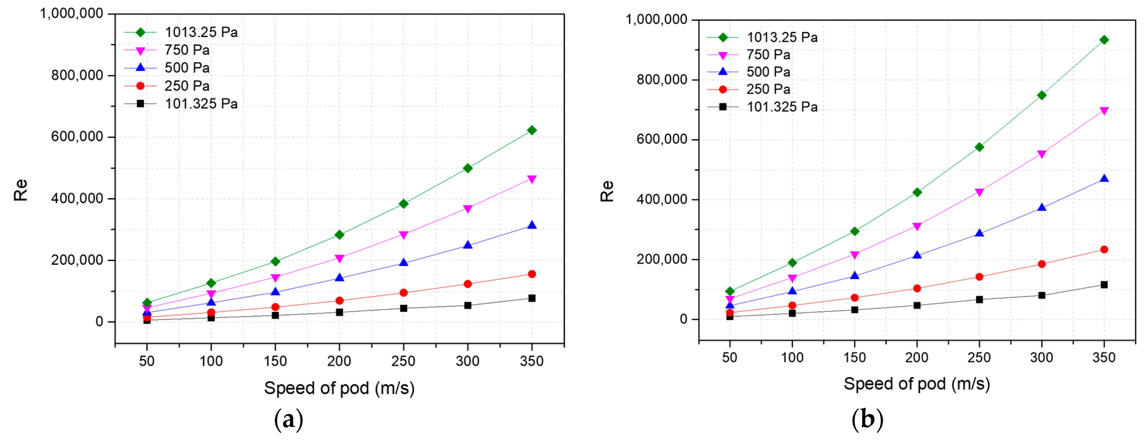
The five main design parameters of the Hyperloop system are the blockage ratio BR, the pod speed and length, and the tube pressure and temperature. To enable a comprehensive analysis of the drag on the pod, simulations were conducted over a large parameter space covering various BR (0.25, 0.36), pod speeds (50–350 m/s), pod lengths (10.75–86 m), tube pressures (101.325–1013.25 Pa, equivalent to 0.001–0.01 atm), and tube temperatures (275–325 K). The study objectives with regard to these parameters are presented below.

(1)

Comparison and validation of drag between two-dimensional axisymmetric and three-dimensional models.

(2)

Pod: the influence of BR, pod speed, and pod length.

(3)

Tube: the effects of the tube pressure and temperature.

In addition, the change in drag because of parametric differences was normalized with respect to the total drag, pressure drag, and friction drag. This relationship can be written as:

$$\mathrm{Drag}=D_T=D_p+D_f,$$

(8)

where $D_T$ is the total drag, $D_p$ is the pressure drag, and $D_f$ is the friction drag; pressure drag is mainly affected by the body shape and flow separation, and friction drag is affected by boundary layer properties such as surface roughness, viscosity, and Re.

3.1. Validation

The reliability and accuracy of numerical CFD (Computational Fluid Dynamics) results can be enhanced by using more suitable turbulence models for certain types of simulations. High-fidelity turbulence simulations, such as direct numerical simulation (DNS) and large eddy simulation (LES), effectively depict detailed dynamics of complex fluid motion, but at the cost of high computational loads [26,27,28,29,30]. To balance the cost and performance of the calculations, the Reynolds-averaged Navier–Stokes (RANS) model (𝑘 − ε, 𝑘 − 𝜔, SST ω, etc.) is widely adopted in compressible flow simulations. In particular, transition SST viscous model is capable of predicting complex transitional flows in fluid motion [31].

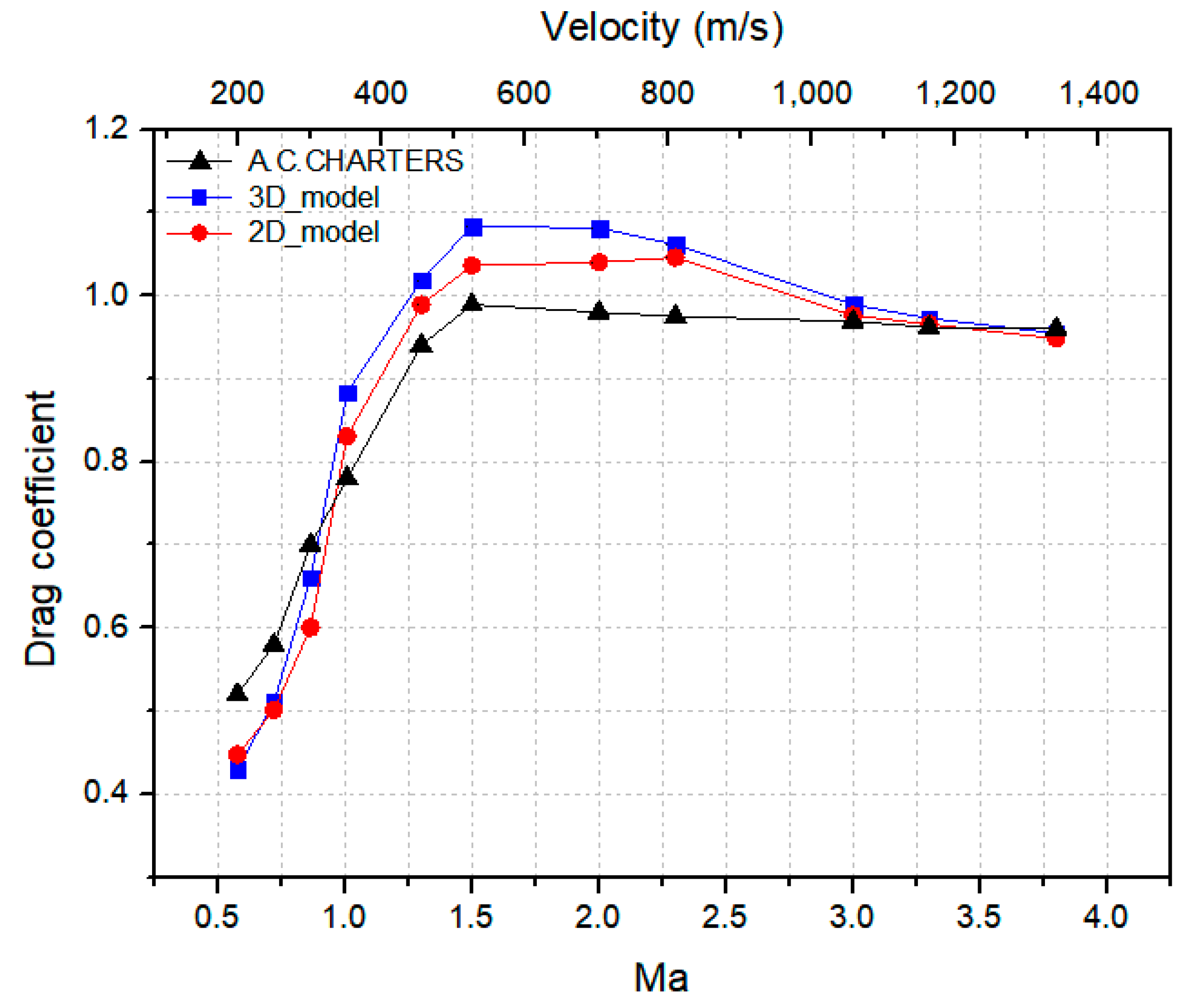
For validation, a steady-state, two-dimensional axisymmetric model was used to determine more suitable turbulence and numerical models. This choice of model was based on previous studies showing that the results obtained in both two-dimensional axisymmetric and three-dimensional simulations do not differ significantly. Such models were created as computationally reconstructed versions of the experimental equipment used by Charters [32], who tested the drag coefficient of a fixed-diameter sphere with respect to variations in speed. The drag coefficient is formulated as:

$$C_D=\frac{D_T}{\frac{1}{2}\rho U^2\frac{\pi }{4}{D}^2},$$

(9)

where $D_T$ is the total drag, D is the diameter of the sphere, and $C_D$ is the drag coefficient. The drag coefficient is a dimensionless number used to quantify the resistance of an object in a fluid environment. Figure 3 shows the comparison between Charters’ experimental data and the drag coefficients obtained in this study from two-dimensional axisymmetric and three-dimensional models. The difference between the two-dimensional axisymmetric and the three-dimensional models is approximately 4%. Similar trends can be observed in the overall results, with the maximum drag occurring at a Mach number of ~1.4 before decreasing to a saturated drag of ~0.9. Thus, we confirmed that the two-dimensional axisymmetric model is appropriate for simulating the Hyperloop system.

3.2. Effects of BR and Pod Speed

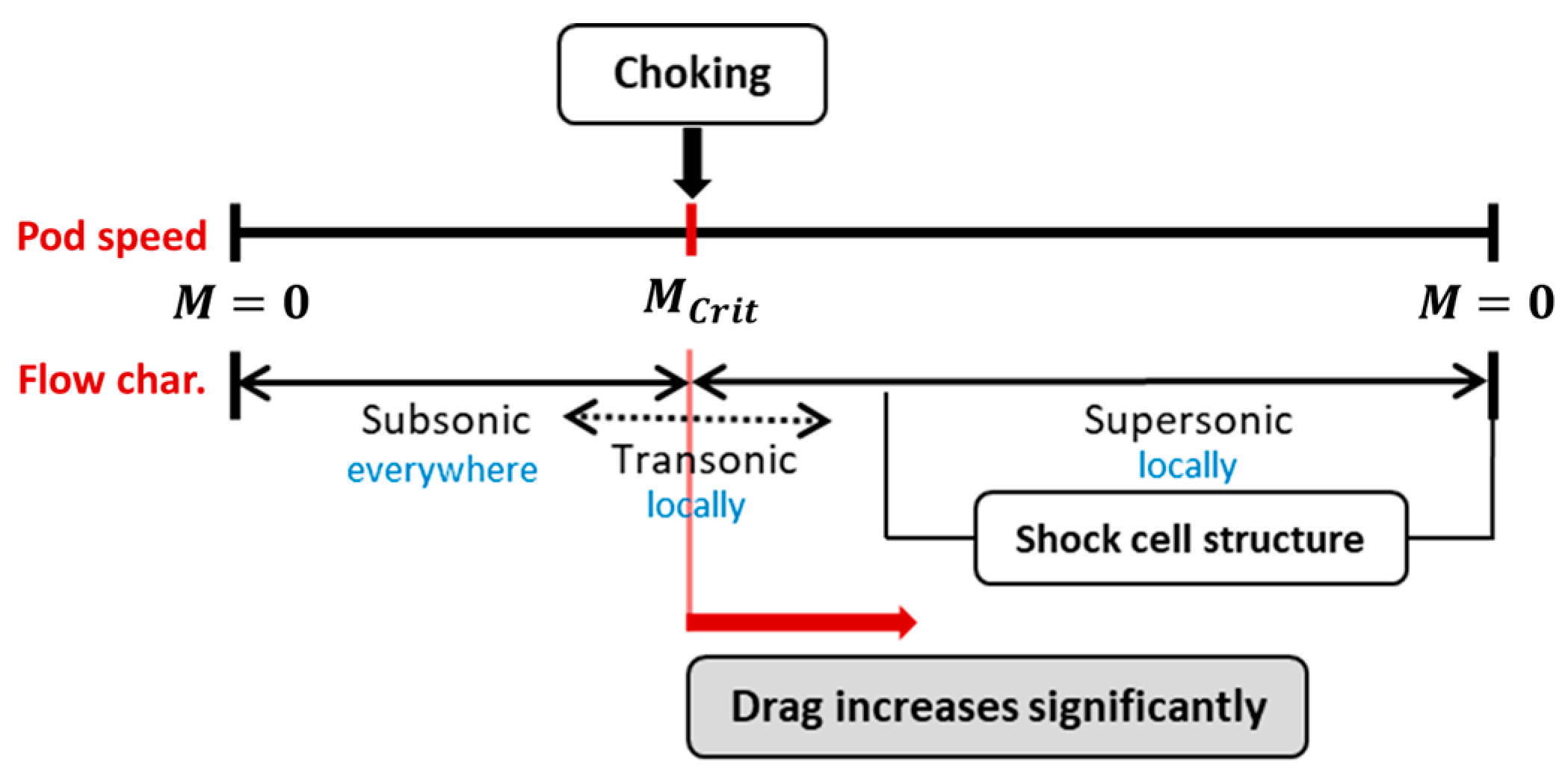
The critical Mach number is the speed at which the choked flow occurs. Beyond this speed, the flow domain can include a supersonic region. When the Mach number is locally greater than 1, a shock wave can appear, leading to a rapid increase in drag, as seen in Figure 4. This phenomenon of the Hyperloop system is similar to converging-diverging nozzles. This allows conventional isentropic gas relations to be applied in calculating the critical Mach number of the Hyperloop system. The critical Mach number of the nozzle can be calculated assuming isentropic flow. Although isentropic flow conditions cannot be applied under real air/friction conditions [33,34], such simplified assumptions deepen our understanding of the actual compressible flow phenomena of shock waves and subsonic-to-supersonic transitions [35,36,37].

In this study, the critical Mach number is calculated using the assumptions stated above. In the Hyperloop system, the critical Mach number varies with BR according to:

$$\frac{A_{tube}}{A_{bypass}}=\frac{1}{Ma}{\left\{\frac{1+\left[\left(\gamma -1\right)/2\right]M{a}^2}{1+\left[\left(\gamma -1\right)/2\right]}\right\}}^{\frac{\gamma +1}{\left[2\left(\gamma -1\right)\right]}},$$

(10)

where $A_{bypass}$ is the cross-sectional area of the bypass region between the tube and the pod, $A_{tube}$ is the cross-sectional area of the tube, Ma is the Mach number of the flow, and γ ($=c_p/c_v$) is the isentropic expansion factor ($c_p$ and $c_v$ are the specific heats of the gas at constant pressure and volume, respectively).

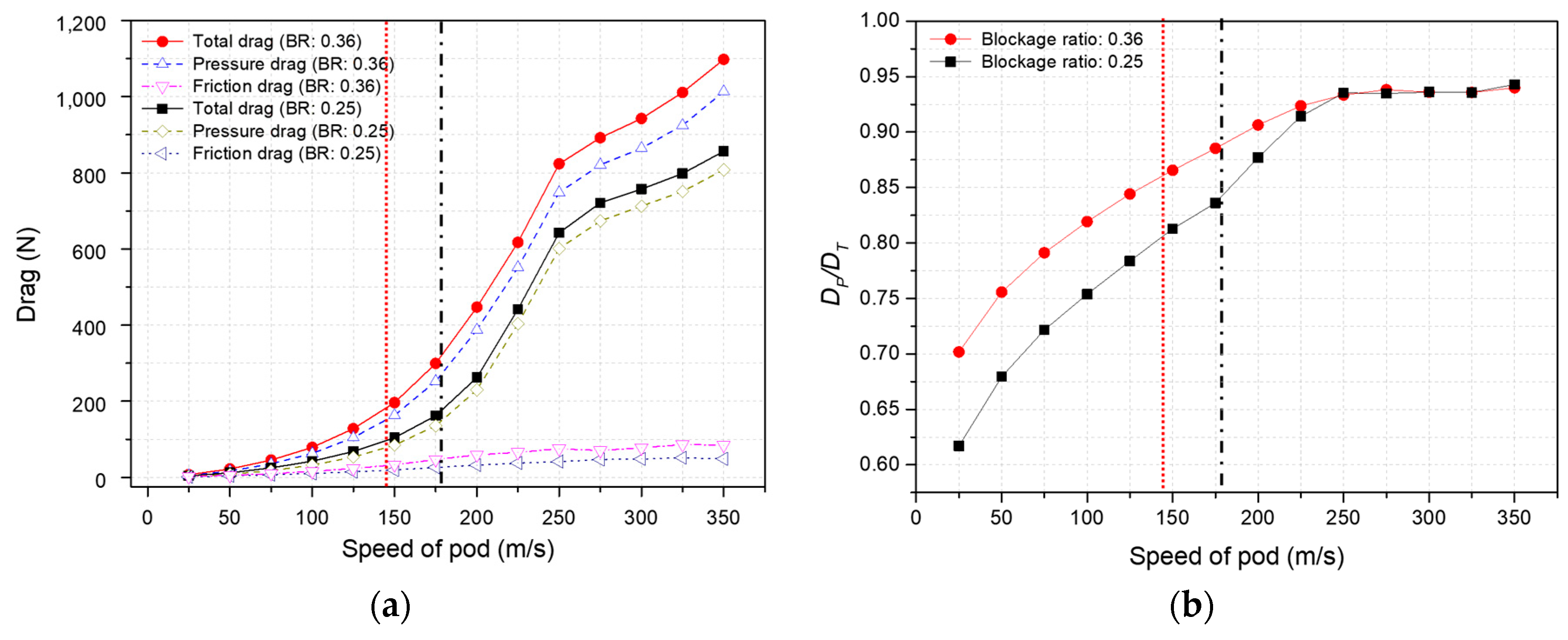
The BR values $\left(A_{pod}/A_{tube}\right)$ used in the case studies were 0.25 and 0.36 (area ratio), corresponding to critical Mach numbers of 0.50 (black dash-dot line) and 0.41 (red dash line), respectively. Hence, BR is inversely proportional to the critical Mach number. Equation (10), however, was based on one-dimensional isentropic assumption. The present CFD had two-dimensional effects which made the critical Mach number of the present study higher than that of a one-dimensional study. Figure 5 shows the effects of BR on the drag. Figure 5a shows the change in total drag, pressure drag, and friction drag with respect to BR. The changes in drag exhibited a similar tendency. First, as BR increased, the influence of the drag on the pod increased. As the speed increased, the drag increased. Second, when BR = 0.36, there was a significant increase at 200 m/s (225 m/s for BR = 0.25) near the end of the pod. Third, we can confirm that the slope of the drag decreased above 250 m/s. This phenomenon was related to the result in Figure 5b, which showed the ratio of total drag to pressure drag. As the pod speed increased, the pressure drag increased proportionally, with the larger blockage ratio enhancing the influence of the pressure drag. This is because of the increase in pressure difference between the nose and end of the pod, followed by the increase in pod speed. However, at speeds above 250 m/s, the pressure drag converged to a certain value, irrespective of BR. Beyond the critical Mach number, the choking phenomenon was very severe, meaning that differences in BR did not have a significant effect on the ratio of the pressure drag to the total drag.

3.3. Effects of Pod Length

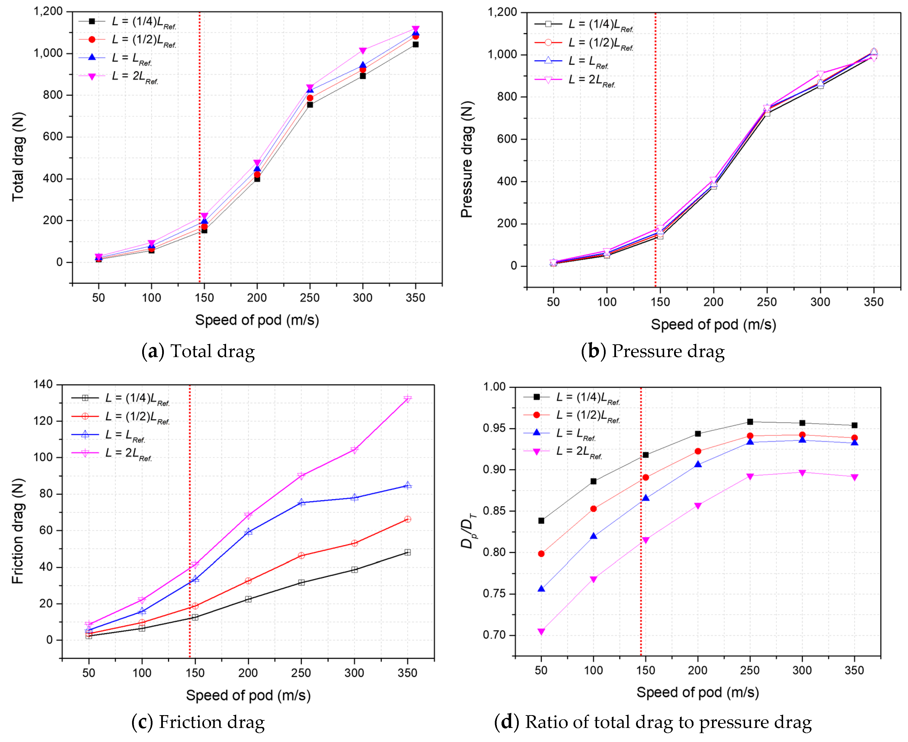
Previous studies only investigated pod lengths of less than 43 m. However, this would restrict the pods to transporting a maximum of 28 passengers. The Hyperloop Alpha document suggests that with 28 passengers at approximately 2-min intervals, Hyperloop could transport 840 passengers per hour to their destination. However, this condition is very energy inefficient and presents a high risk of accidents. Therefore, it is necessary to increase the pod length and investigate the effect of the length on the drag. In this study, the pod length was set to 10.75 m, 21.5 m, 43 m, or 86 m, and the change in drag was analyzed. Figure 6 shows the change in drag with respect to pod length. Figure 5b and Figure 6a confirm that the total drag and pressure drag are almost insensitive to pod length. However, the friction drag is proportional to pod length (Figure 6c). As the influence of the pressure drag does not change, the ratio of total drag to pressure drag decreases (Figure 6d). This is because the friction drag is mainly influenced by the surface area. As a result, changes in the pod length do not significantly affect the drag, as most of the drag is caused by the pressure.

3.4. Shock-Cell Structure

As mentioned above, the geometrical features of the Hyperloop system are similar to those of conventional converging-diverging nozzles, which exhibit well-known complex flow phenomena such as choking and shock waves. One of the most important supersonic flow phenomena, shock waves, occurs when the fluid moves faster than the speed of sound. They are discontinuous and difficult to control, rapidly changing the flow fields of pressure, temperature, and density. 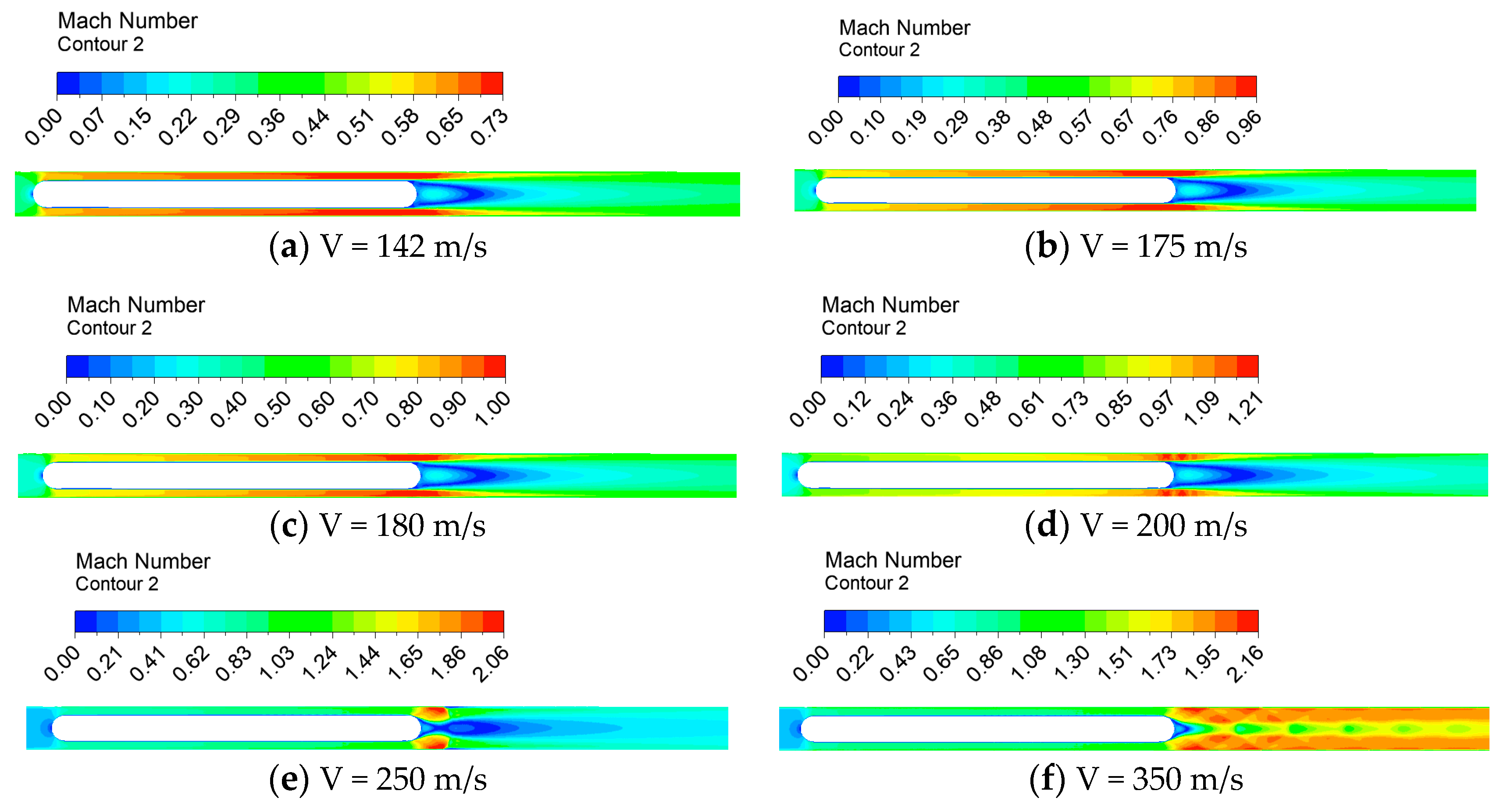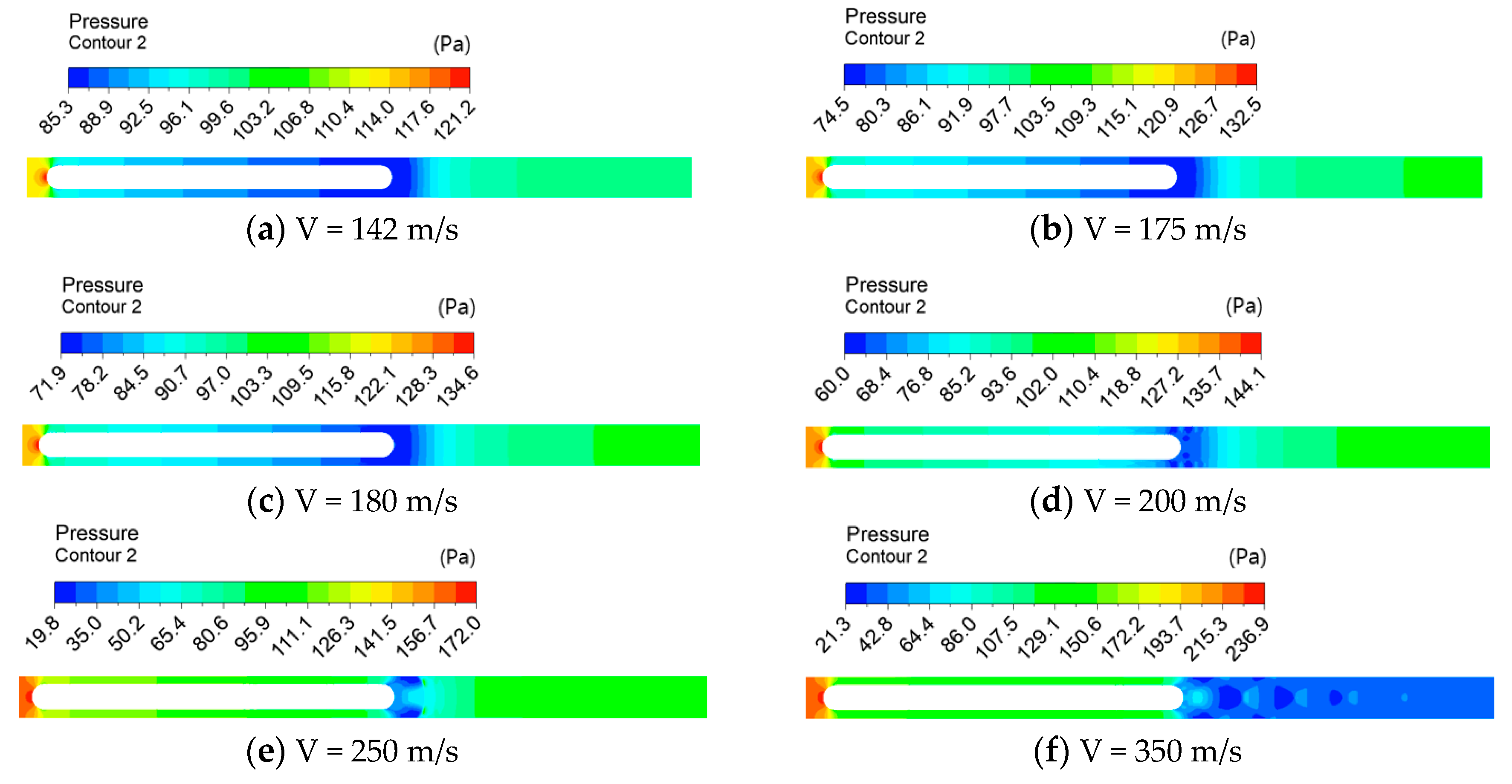Figure 7 and Figure 8 show the variations in Mach number and pressure with respect to pod speed. Flow velocity reached a Mach number of 1 at the pod speed of V = 180 m/s (Ma = 0.52). The critical Mach number calculated from Equation (10) was 0.41 (V = 142 m/s), which is lower than the one obtained from present two-dimensional simulation. This difference in value is because of the two-dimensional nature of the present Hyperloop study. Shock waves were observed at a pod speed of V = 200 m/s at the end of the pod, and became more distinguishable when V = 250 m/s. The strong shock-cell structure at the end of the pod was caused by severe choking of the flow around the pod. This explains the convergence of the ratio of pressure drag to total drag described in Section 3.2. In conclusion, as the pod speed increases, the pressure difference between the nose and the end of the pod increases; however, once the choking phenomenon occurs, the ratio of pressure drag to total drag gradually converges to ~0.93.

3.5. Effects of Tube Pressure

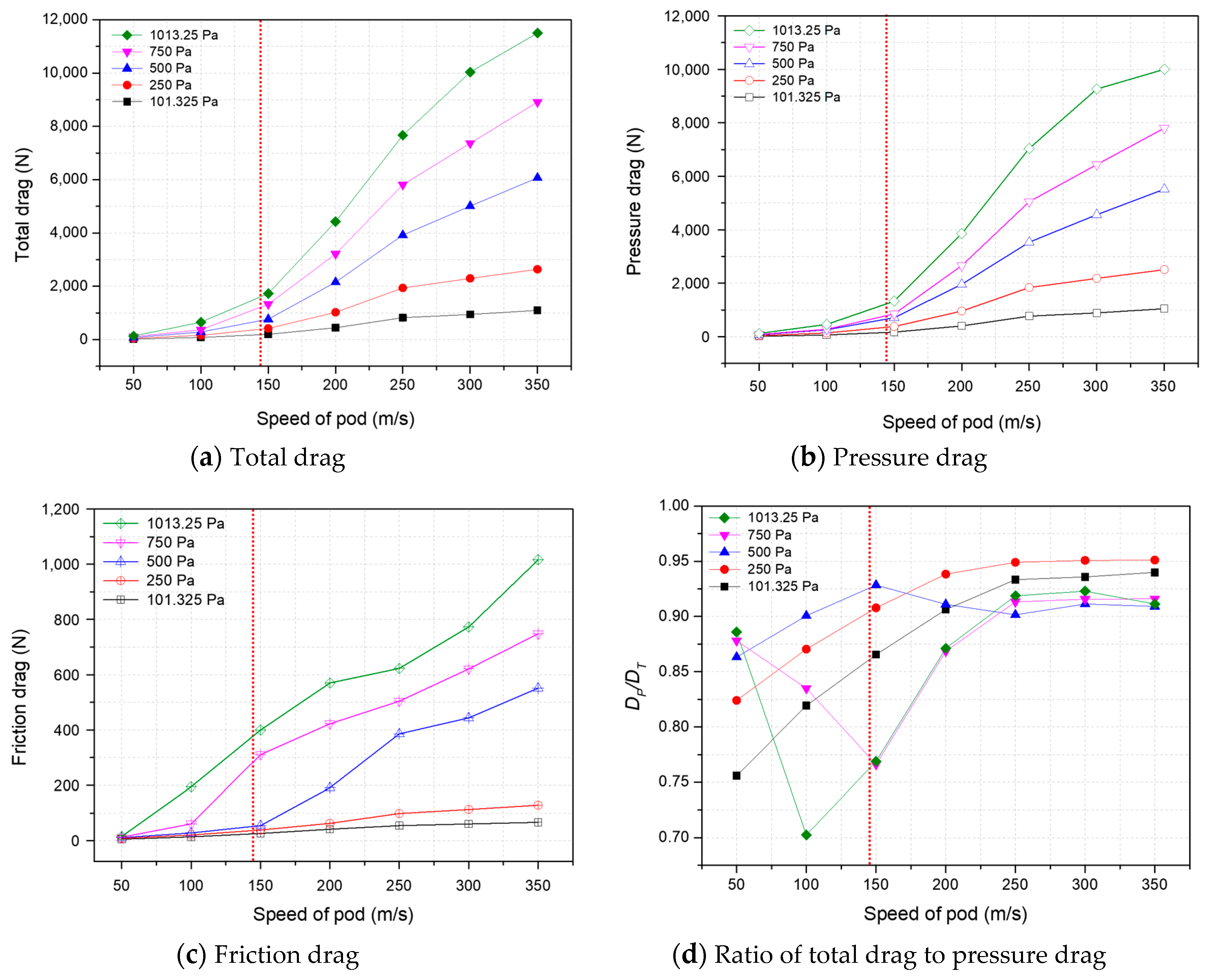
The target tube pressure of the Hyperloop system is 101.325 Pa (0.001 atm). This is because a lower tube pressure corresponds to lower drag on the pod. In this study, we analyzed how the change in pressure affects the drag on the pod. Figure 9 shows the variation in drag with pressure changes at BR = 0.36. The total drag, pressure drag, and friction drag all increased with increasing pressure, as shown in Figure 9a–c. Interestingly, the friction drag exhibited a slightly different tendency. Generally, the friction drag increases slightly with increasing pod speed at 101.325 Pa and 250 Pa. However, at pressures above 500 Pa, the friction drag increased significantly at low speeds. At 500 Pa, the friction drag increased rapidly above 200 m/s, while 750 Pa and 1013.25 Pa produced rapid increases above 100 m/s. Figure 9d shows the ratio of total drag to pressure drag at various pressures. The effect of the pressure drag caused this ratio to increase with a similar trend at 101.325 Pa and 250 Pa. However, the effect of friction drag increased at around 200 m/s when the pressure was at 500 Pa. At higher pressures, the influence of the friction drag increased significantly above 100 m/s, and the effect of pressure drag gradually increased as the speed increased.

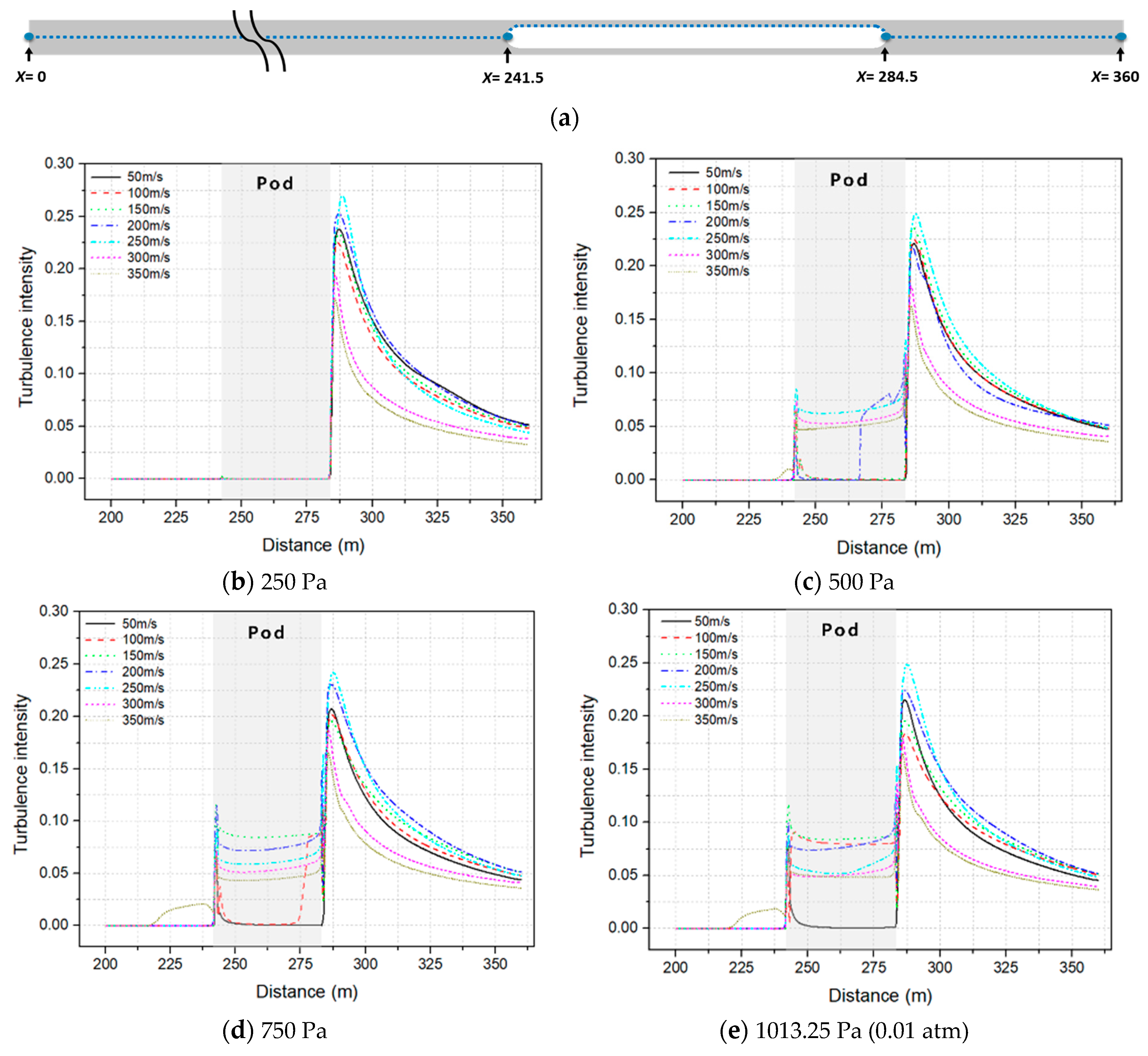
To confirm the above phenomenon, we examined the turbulence intensity. Figure 10 shows the turbulence intensity for each pressure along the line in Figure 10a. For 101.325 Pa and 250 Pa, the results exhibited a similar trend. The turbulence intensity increased significantly at the end of the pod, but did not directly affect the pod. The reason is that the drag measured here was the mean value of the drag applied to the surface of the pod, and the turbulence intensity increased at the end of the pod. However, the turbulence intensity increased at the pod surface at pressures greater than 500 Pa. At 500 Pa, the turbulence intensity on the surface increased significantly at the center of the pod at speeds of 200 m/s. In addition, the turbulence intensity increased at the back of the pod at speeds of 100 m/s with a pressure of 750 Pa, and significantly increased at all pod speeds, except for a speed of 50 m/s, when the pressure was 1013.25 Pa. This increase in turbulence intensity and friction drag on the surface of the pod were caused by increases in the tube pressure, density, and Re.

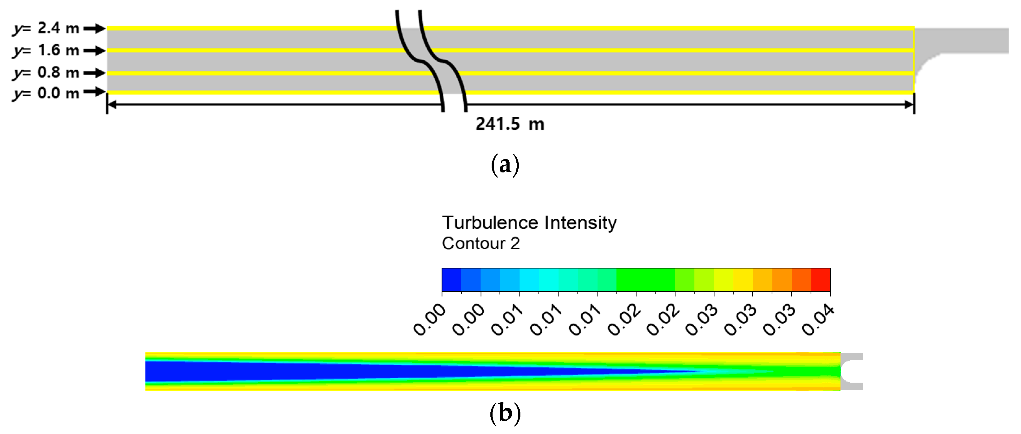
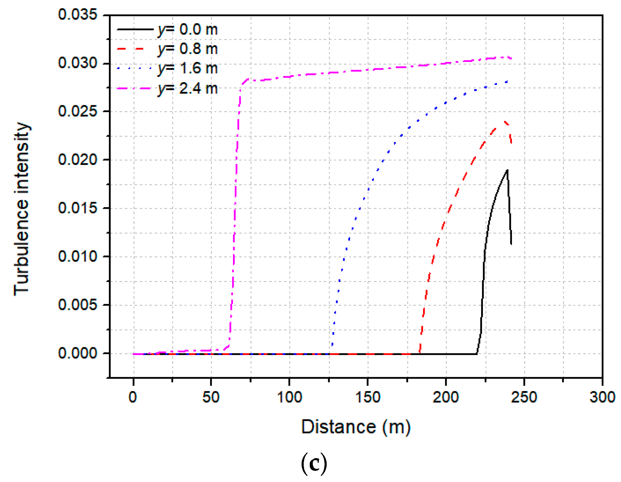
In Figure 10, turbulence intensity at the frontal region of the pod started to increase at a pod speed of 350 m/s and tube pressure of 500 Pa. This is because of a strong turbulence occurring near the tube wall at the front of the pod. Such turbulence was generated due to the relative difference in flow velocity at and near the wall. At relatively low pod speed range, flow velocity at and near the wall were the same. However, at relatively high pod speed range this difference becomes greater, causing stronger turbulence (Figure 11). The frontal region of the pod is affected by compression waves and choking. These phenomena have a significant impact at high-pressure and high-speed (above critical Mach number) conditions, resulting in an increase in pressure at the front of the pod. This accelerates the relative velocity difference between the tube wall and near-wall flows at the frontal area of the pod. The starting point of this turbulence propagates in upstream direction as y-value moves towards the wall. Information shown in Figure 11 is depicted based on conditions of tube pressure 1013.25 Pa (0.01 atm) and pod speed of 350 m/s.

3.6. Energy Cost to Overcome Drag

An additional simulation was conducted as a control case, whereby the pod travelled in atmospheric conditions without the tube. The aim of this simulation was to determine the economic efficiency of the near-vacuum tube installation. The results were compared with a Hyperloop system under a tube pressure of 101.325 Pa and identical pod speeds of 350 m/s, with an assumed travel time of 15 min (traveling approximately 315 km). The results in

Table 2. Energy cost comparison between the control case (101.325 Pa with open space) and 101.325 Pa Hyperloop case at a pod speed of 350 m/s for 15-min operation (315 km movement). The cost is calculated assuming that the electricity is ideally converted to thrust to overcome the drag with perfect efficiency.

Pressure	Drag (N)	kWh	Cost ($)
101.325 Pa (1 atm, open space)	407,553	35,661	7011
101.325 (1/1000 atm, tube)	1098	96	20

indicate that the control case generated a drag of 407,553 N and required 35,661 kW, whereas the Hyperloop system had a drag of 1098 N and required only 96 kWh. The electricity cost was $7011 for the control group and $20 for the Hyperloop system, based on the KEPCO (Korea Electric Power Corporation) energy charges and assuming fully efficient usage of the energy to overcome the drag [38]. Other external factors such as maintaining the pressure in the tube were not considered in the calculation. Experiments and tests conducted at the Korea Railroad Research Institute concluded the initial cost of vacuum creation and maintaining a specific vacuum pressure when installing a steel to be inexpensive (pump equipment, electricity costs, etc). These results show that the energy cost required to overcome the drag is approximately 350 times greater in the control case than in the Hyperloop system under a tube pressure of 101.325 Pa. Hence, the near-vacuum tube greatly reduces the energy cost for high-speed transportation.

3.7. Effect of Temperature

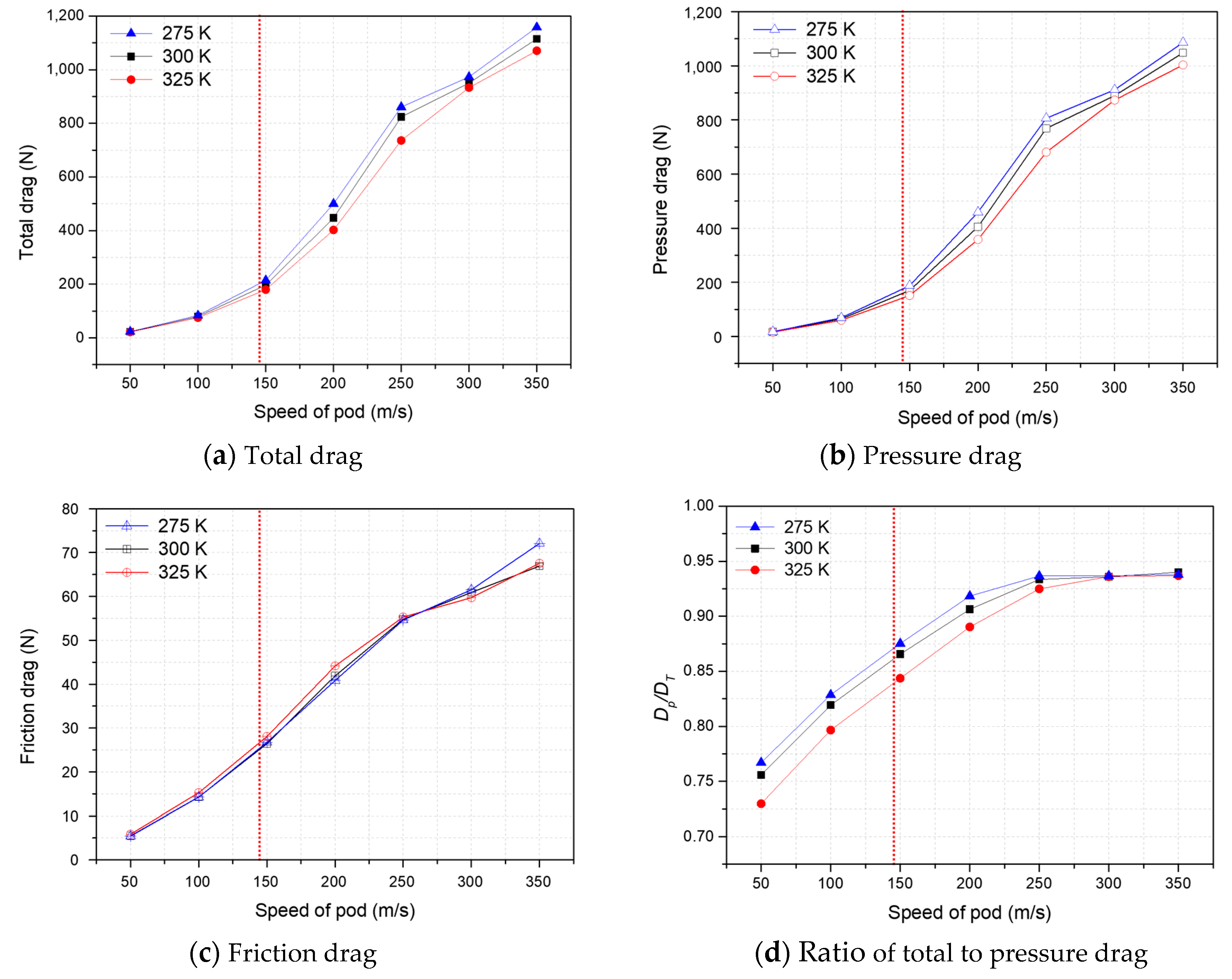
The change in drag resulting from changes in temperature has not been considered in previous studies. In fact, changes in temperature are an important factor in the transonic-speed operation of the Hyperloop system. The tube temperature affects parameters, such as the speed of sound, density, and viscosity, that have a significant impact on drag. Figure 12 shows the variation in drag with respect to temperature. In Figure 12a, the total drag applied to the pod decreases as the temperature increases. The reason for this decrease is that the pressure drag decreases with increasing temperature (Figure 12b). As the tube temperature increases, the speed of sound increases. Hence, the Mach number decreases for the same pod speed, and therefore, the pressure drag decreases. The change in drag according to this temperature change is only significant for the pressure drag, with the friction drag relatively unaffected. It can be seen that the ratio of total drag to pressure drag tends to converge above 300 m/s for higher temperatures. In Figure 4, convergence occurred at 250 m/s. This is because the severe choking was delayed by the increase in tube temperature. As a result, the drag decreased as the temperature increases. However, the increase in temperature outside the pod may lead to increased energy consumption to maintain the pod’s internal temperature. Considering the small differences in drag caused by temperature changes, it is relatively inefficient to increase the tube temperature as a means of reducing the drag.

4. Conclusions

In this study, numerical simulations have been performed to analyze the flow characteristics present in the Hyperloop system using a two-dimensional axisymmetric model. We focused on the aerodynamic drag, which is one of the most important parameters in the Hyperloop system. The effects of the changes in the blockage ratio, pod speed, pod length, tube pressure, and tube temperature have been investigated, and flow phenomena such as choking and shock waves near the pod were considered.

The primary findings are as follows. First, as the blockage ratio increases, the drag on the pod becomes greater because of the smaller critical Mach number. Second, as the pod speed increases, the overall drag increases. For a tube pressure of 101.325 Pa, the drag increases from 7.42 N at a pod speed of 25 m/s to 1098.60 N at a pod speed of 350 m/s. In particular, the drag significantly increases when the pod reaches the critical Mach number. Strong shock waves begin to occur at 200 m/s for BR = 0.36 and at 225 m/s for BR = 0.25 near the end of the pod. Above this speed, the flow around the pod becomes severely choked at both BR values, and the ratio of the pressure drag to the total drag converges to its saturation level. Third, changes in the length of the pod do not significantly affect the total and pressure drag, but strongly affect the friction drag. Fourth, the tube pressure and drag show a proportional relationship. Specifically, the friction drag increases rapidly as the tube pressure increases. This is due to more energetic turbulence at higher-pressure (and higher-density) flow, which is confirmed by the enhanced turbulence intensity along the pod surface. Finally, high tube temperatures increase the speed of sound, thus reducing the Mach number for the same pod speed and delaying the onset of choking. This reduces the aerodynamic drag. These results are applicable for the fundamental design of the proposed Hyperloop system.

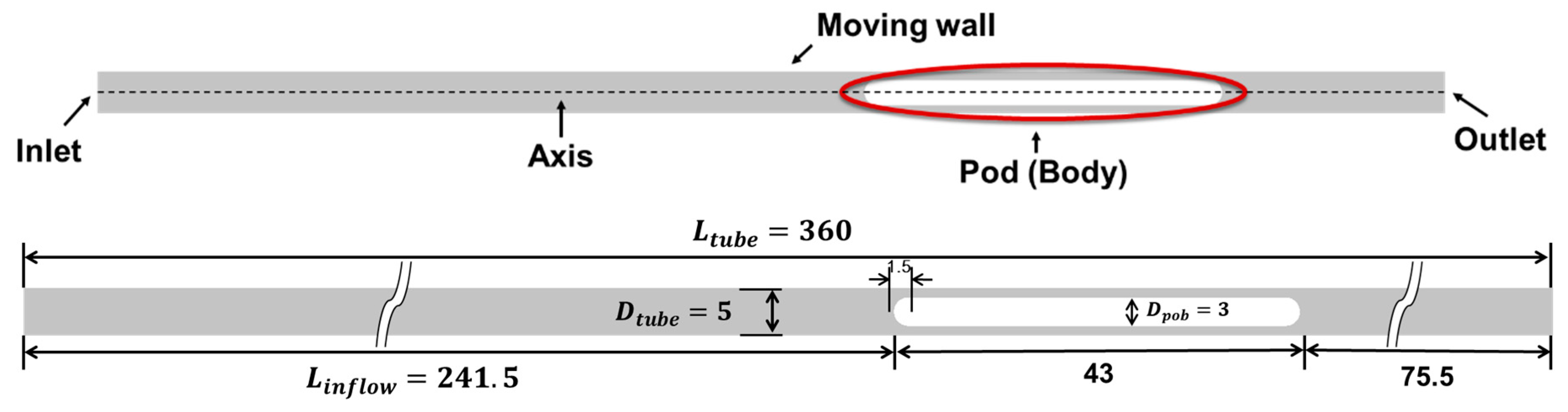
This study performed CFD simulations of a Hyperloop system over a large parameter space with an idealized axisymmetric computational domain created based on actual measurements of pod length, diameter, and tube diameter. However, our steady-state two-dimensional simulation only presents converged results of transitional changes. For this reason, we have focused on the effects that are not significantly affected by transient and three-dimensional characteristics of the system. In future studies, unsteady and three-dimensional simulation would be more suitable for clear representation of the propagation of compression wave and complex pod shape potentially based on the present results.