Towards the EU Emission Targets of 2050: Cost-Effective Emission Reduction in Finnish Detached Houses

Abstract

To mitigate the effects of climate change, the European Union calls for major carbon emission reductions in the building sector through a deep renovation of the existing building stock. This study examines the cost-effective energy retrofit measures in Finnish detached houses. The Finnish detached house building stock was divided into four age classes according to the building code in effect at the time of their construction. Multi-objective optimization with a genetic algorithm was used to minimize the life cycle cost and CO₂ emissions in each building type for five different main heating systems (district heating, wood/oil boiler, direct electric heating, and ground-source heat pump) by improving the building envelope and systems. Cost-effective emission reductions were possible with all heating systems, but especially with ground-source heat pumps. Replacing oil boilers with ground-source heat pumps (GSHPs), emissions could be reduced by 79% to 92% across all the studied detached houses and investment levels. With all the other heating systems, emission reductions of 20% to 75% were possible. The most cost-effective individual renovation measures were the installation of air-to-air heat pumps for auxiliary heating and improving the thermal insulation of external walls.

1. Introduction

European Union (EU) climate goals aim to reduce greenhouse gas emissions by 80% by 2050, compared to the level of 1990 [1]. Energy use in buildings accounts for 40% of energy consumption and a similar fraction of greenhouse gas emissions in the European Union (EU). This is why the Energy Performance of Buildings Directive (EPBD) requires all new houses to be nearly zero-energy buildings by the end of the year 2020. In addition, the latest update to the EPBD calls for all EU member states to create a roadmap for the energy renovation of existing buildings as well. [2]. The requirement to improve building energy efficiency alongside other renovations has also been outlined in Finnish environmental regulation [3].

In Finland, 79% of buildings (according to the heated net area) were constructed before the year 2000, which highlights the need to focus on the existing building stock [4]. Detached houses make up 34% of all Finnish built floor area, with row houses accounting for another 7%. Together they make up 190 million square meters of heated floor area. Energy retrofit of these buildings can have a great effect on Finnish carbon emissions. In this vein, [5] showed that final energy use in Swedish detached houses could be reduced by 65%–75%. The aim of this article is to examine the retrofit potential in a Finnish context.

To drive the renovation of old residential buildings, a tool for retrofitting design was presented in [6]. The tool utilized preferences given by the user and then ranked different solution packages according to the importance given for different categories (environmental, economic, social). Another such tool was the monthly-based energy auditing tool presented by [7]. While not requiring much expert knowledge, it was able to estimate heating and cooling demands in several climates within 8% to 15% of a more detailed dynamic simulation tool, TRNSYS [8]. However, another study compared the energy efficiency improvements of a simple single zone model to those realized in an actual building and found out the real heating demand was up to 50% higher than the simulated demand [9]. The use of a more detailed multi-zone modeling was suggested. Simplified building modeling was also used in [10], where the whole German energy system was simulated in detail, but the retrofit of buildings was estimated by simple interpolation on a line with an assumed cost to energy savings ratio. To achieve the decarbonization of the whole energy sector in Germany required a 60% reduction in building energy use [11]. This highlights the importance of more detailed calculations in the building sector to find the best ways to reach the targets.

While estimating current energy use and testing pre-selected renovation packages can be beneficial, perhaps the most effective tool for designing building retrofits is to use multi-objective optimization, where many design variables can be freely changed to iteratively achieve an optimal retrofit solution. This has been utilized for old Finnish apartment buildings to minimize life cycle costs and primary energy use [12] or carbon emissions [13]. In a Korean study, a genetic algorithm (GA) was used for the optimization of the energy system of an elementary school [14]. Only heating and cooling systems were retrofitted, without any changes to the building envelope. Three objectives, life cycle cost, renewable energy penetration, and greenhouse gas emissions, were used in the optimization. A pairwise comparison between two objectives was used to help with the challenge of having three objectives. A genetic algorithm was also used in a Canadian case, where further efficiency improvements were planned to improve an old house that had already been improved before [15]. Three objectives were split into two separate optimizations, life cycle cost vs. peak load and life cycle cost vs. energy savings with the aim of improving building energy performance above minimum requirements of the national code. The two different objectives resulted in different focus points for the retrofit, even though their principal goal of environmental benefits was the same. It is also possible to combine multiple objectives into one by calculating the weighted sum of all the objectives. This was used in [16] to optimize the retrofit of building envelope and solar panels.

A Portuguese study examined the optimal retrofit of houses set in four different regions in Portugal [17]. Using a GA, the envelope and mechanical systems were optimized to maximize energy savings and minimize initial investment cost. The rebound effect was considered by reducing the realized savings from upgrades. The importance of simulation zones and energy use profiles was studied in [18]. Optimal retrofit configurations remained the same regardless of user profiles, but the achieved energy savings obtained by each configuration did change.

When deep renovation of old detached houses was studied in Estonia, the installation of mechanical ventilation with heat recovery was found to be the most effective energy retrofit option [19]. Adding thermal insulation to external walls proved to be too costly. A study made on many types of detached houses in Chicago revealed that most homes could have their energy consumption reduced by 50% over a 25-year payback period [20]. Optimization was made by targeting the most cost-effective configurations, i.e., by finding the highest savings per cost ratio. The optimization was made in two steps, first to optimize the envelope, then to optimize the energy system. In this case, wall insulation was deemed economical. Ekström et al. [21] reported that the cost-effectiveness of detached house energy retrofitting in Sweden was dependent on the heating system of the house. Generally, installing exhaust air heat pumps was cost-effective, while window retrofitting was not. Renovation up to passive house standards was cost-effective in houses with direct electric heating. Heat pumps have generally been found to reduce energy consumption and emissions. In Canadian studies, air-to-water heat pumps reduced the greenhouse gas emissions of the housing stock by 23% [22], while solar-assisted heat pumps reduced emissions by 19% [23]. Here, the key question is how the electricity to run the heat pumps is produced, as larger reductions are achievable with low emission electricity.

Bjørneboe et al. [24] confirmed through a year-long monitoring campaign that simulated energy savings of a renovated single-family house matched those of a real building. Heating energy consumption was reduced by over 50% while improving thermal comfort. In addition, 77% of the renovation expense was covered by an increase in house value. This means that the real cost of energy retrofitting can be lower than typically estimated.

Deep renovation that reduces heating demand can cause a risk of overheating. However, overheating may be reduced by solar shading systems and increased ventilation rates [25]. Another issue with deep renovation is whether it can be practically done. Significant emission reductions in Sweden could be achieved by deep renovation in principle, but reaching passive house levels may not be possible in most cases, due to the design of the building envelope or foundation [5]. Another issue with achieving emission reductions is the embodied energy of building materials. Low operational energy use requires more materials with their own emission footprint. The inclusion of all phases of the building life cycle in the emission assessment is thus suggested [26].

The perceptions of the benefits of energy renovations in Swedish single-family houses were found to vary according to motivation to perform the renovations [27]. The indoor environment was often found to be a more important reason for house renovations than reducing energy consumption. Lack of information and access to low-interest loans were found to impede energy renovation projects. Similar observations were made in a Danish study, which suggested that to increase the prevalence of energy renovation, the focus should be shifted from investment to non-energy benefits [28]. In addition, subsidies should be enhanced, renovation plans should be included in the energy performance certificates, and maximum allowed energy consumption in houses should be regulated. These findings were repeated in another study, which tried to offer energy efficiency packages to building owners [29]. Despite the rational basis of the packages, building owners were better motivated by indoor comfort and easy solutions that might improve the aesthetics or property value. Thus, more acceptable renovation packages were formulated, with less emphasis on energy savings. Similar results were found in a survey of 883 Danish single-family house owners, which emphasized that owners need more information on non-economical and non-energy related renovation possibilities [30]. House owners often lack knowledge of their own energy consumption, which further reduces interest in doing energy retrofits.

Typically, studies on building energy renovation are focused on energy or cost. Often, energy savings are reported without taking into account the energy source. However, there is a strong national aspect to the solutions, as the climate and energy generation infrastructure varies between countries. The novelty in this study is that we minimize greenhouse gas emissions in detached houses by taking into account the emissions of different heating systems and the seasonally variable emissions of electricity in Finland. The building envelopes and technical systems also vary by age and region; thus, there is no single universal solution to be used for every country. In this study, multi-objective optimization is utilized to find a balance between emissions and life cycle cost for deep renovation solutions in Finnish buildings built in different decades. An earlier study used similar methodology to search for cost-optimal solutions to minimize emissions in Finnish apartment buildings [13]. This study will cover the rest of the Finnish residential building stock by finding the emission reduction potential in single-family homes of four different age categories, which has not been done before in Finland. The novelty is in the optimization of a large combination of buildings and heating systems, covering existing buildings of various ages. All the retrofit parameters are adjusted freely without pre-selected packages. The study is part of a larger plan to optimize the deep renovation of all major building types in Finland and estimate the effect on the national energy system.

2. Materials and Methods

2.1. Simulation Setup

The Finnish detached houses were modeled on an hourly timescale using the dynamic simulation tool IDA-ICE [31], which has been validated, for example, in [32,33]. The weather file used in the simulations was the Test Reference Year for Southern Finland (TRY2012-Vantaa). The annual average outdoor air temperature is 5.6 °C, and the annual solar insolation on a horizontal surface is 970 kWh/m² [34]. The heating degree day value for the studied climate zone (at indoor temperature of 17 °C) is 3952 Kd [35].

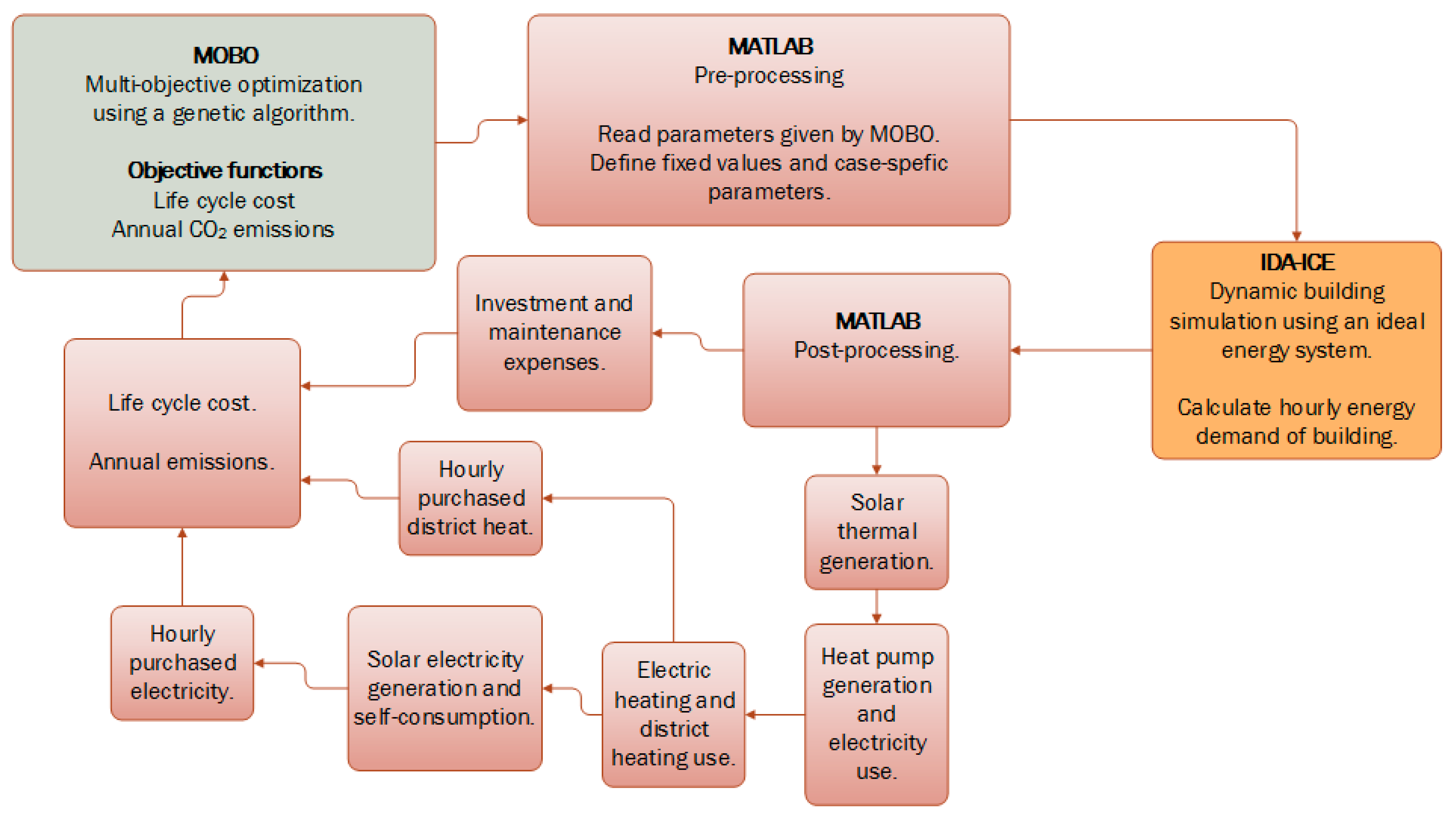
The dynamic building simulation by IDA-ICE was combined with MATLAB for additional pre- and post-processing, and the MOBO tool [36] for multi-objective optimization. The optimization process is shown in Figure 1. The MOBO software runs the optimization loop, which provides trial configurations for building retrofit and feeds them to MATLAB. MATLAB then generates a simulation input file compatible with the building simulation tool IDA-ICE. After IDA-ICE has simulated the building performance, MATLAB calculates the cost and emissions of running the system and returns the answers to MOBO to prepare the next iteration of the optimization.

2.2. Building Descriptions

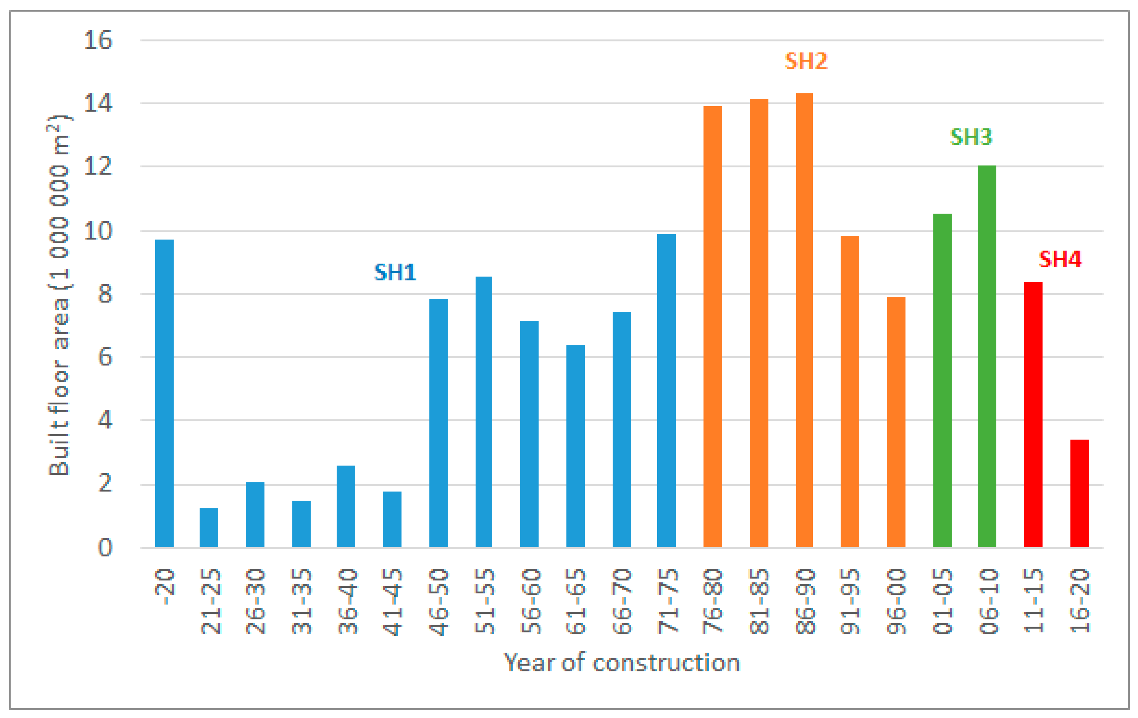
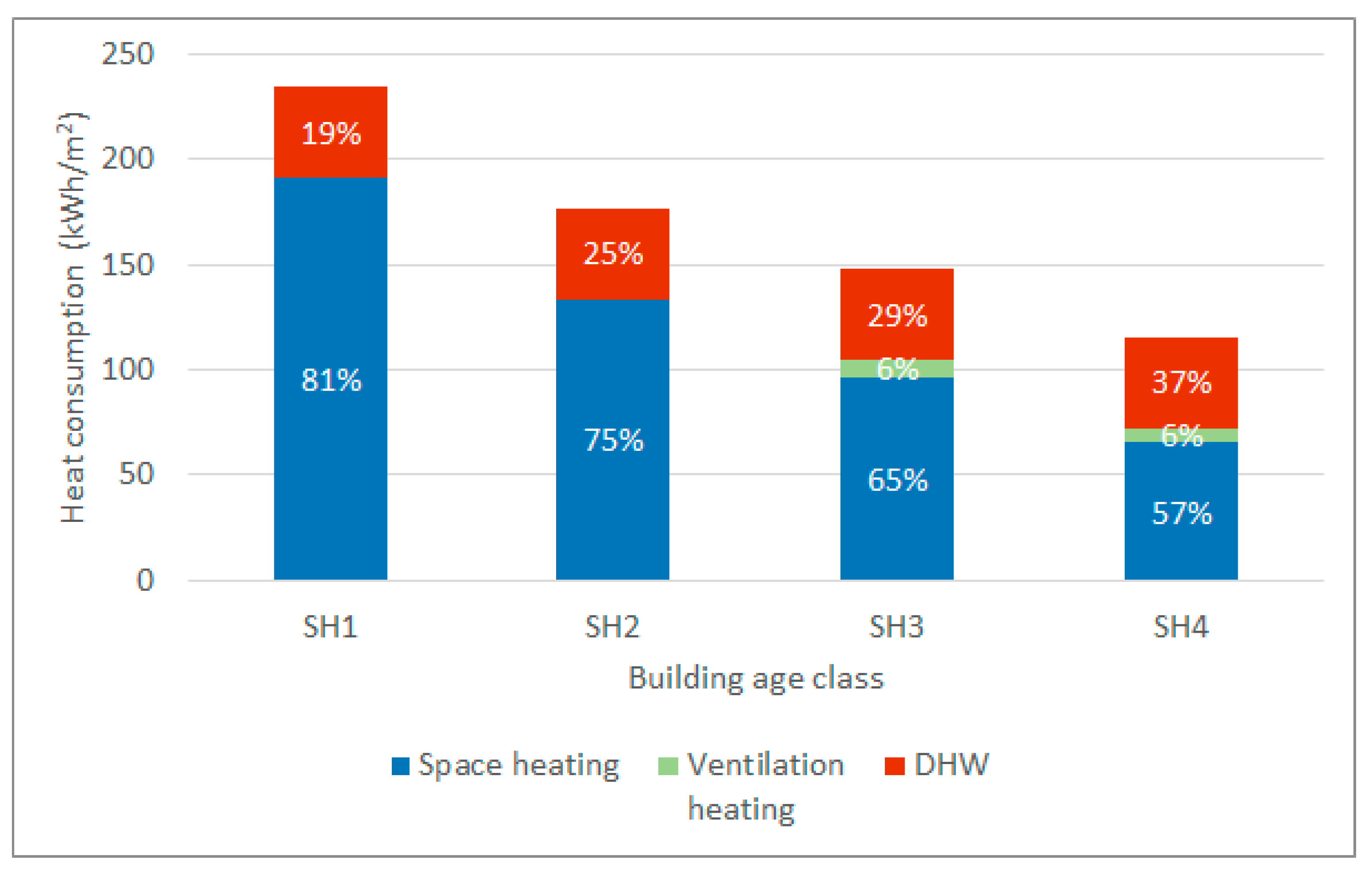
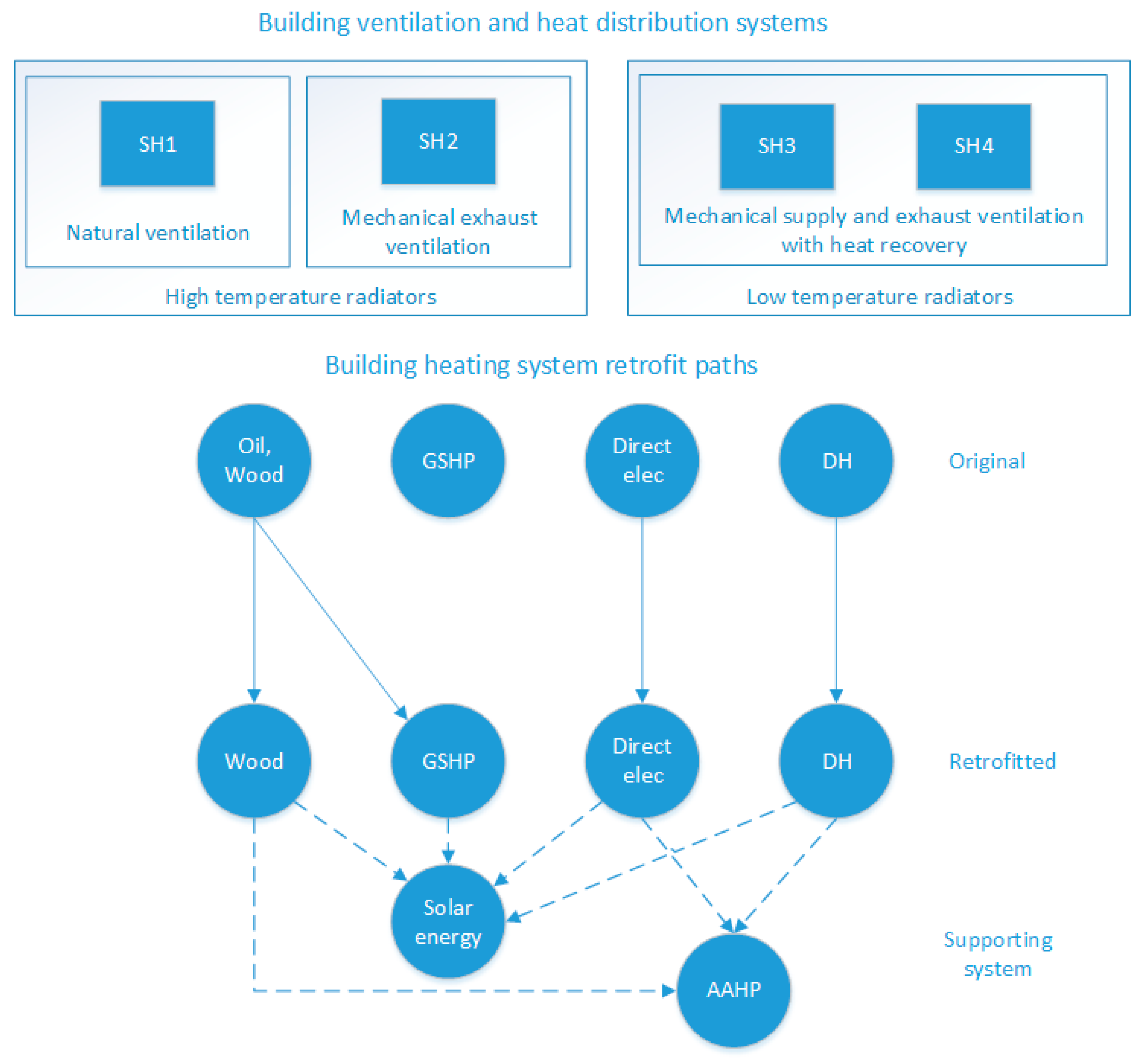
Because residential detached houses account for such a large fraction of Finnish building stock, their effect on national emissions is also great. Figure 2 shows the building stock age distribution for single-family houses (SH) [4]. The buildings were divided into four age categories, according to the Finnish building code of the time. The oldest group SH1 was built before any energy efficiency requirements were issued and is thus poorly insulated and uses natural ventilation. SH2 is a large group of old buildings with slightly improved insulation and mechanical exhaust ventilation (E. vent.) without heat recovery. SH3 is a group of well-insulated buildings equipped with mechanical supply and exhaust ventilation and heat recovery (S. & E. vent.). SH4 is very well insulated and has improved ventilation heat recovery efficiency. The details of the buildings are shown in

Table 1. Properties of the reference single-family houses. [37].

Building Age Class	SH1	SH2	SH3	SH4
Construction years	–1975	1976–2002	2003–2009	2010–
U-values of envelope (W/(m2K))
External wall	0.584	0.28	0.25	0.17
Floor	0.48	0.36	0.25	0.16
Ceiling	0.343	0.22	0.16	0.09
Doors	1.4	1.4	1.4	1.0
Windows	1.8	1.6	1.4	1.0
Total solar heat transmittance (g)	0.71	0.59	0.46	0.46
Direct solar transmittance (ST)	0.64	0.52	0.39	0.39
Air tightness
n50, (1/h)	6	4	3.5	2
q50 m3/(h m2)	15.6	10.4	9.1	5.2
Ventilation
Type	Natural ventilation	Mech. E. vent.	Mech. S.&E. vent.	Mech. S.&E vent.
Heat recovery temp eff	0	0	0.55	0.65
Ventilation rate (L/s/m2)	0.30	0.33	0.36	0.36
Total air exchange rate (1/h)	0.41	0.46	0.5	0.5
SFP (kW/m3/s)	0	1.5	2.5	2
Heating setpoint (ºC)	22	22	21.5	21

.

2.3. Building Service Systems

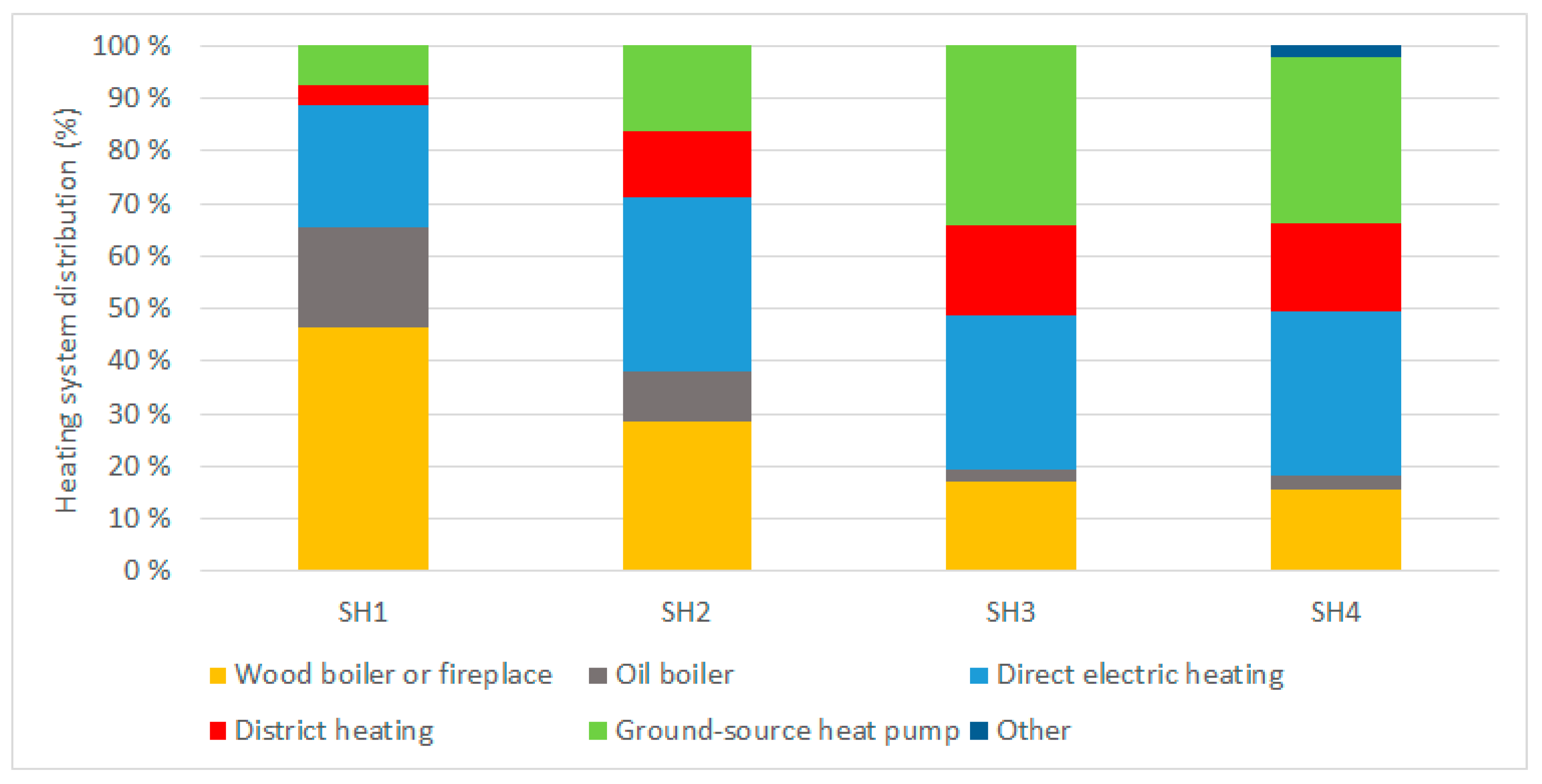
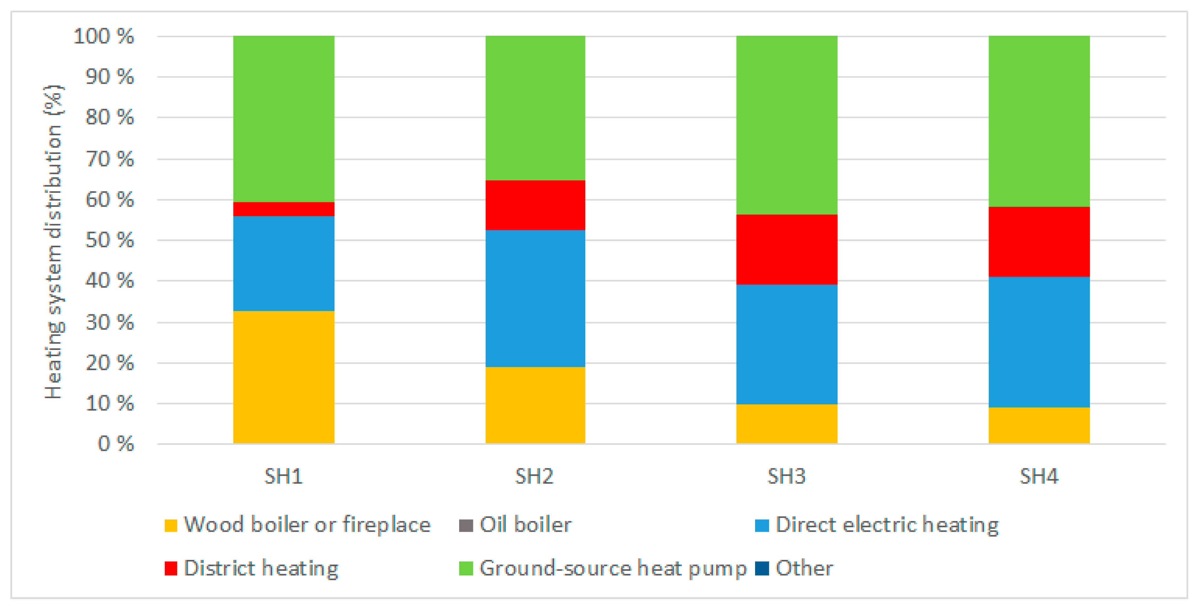
The main heating systems used in single-family houses in Finland are shown in Figure 3. The information is based on the registry information from Statistics Finland but does not contain possible changes that have been made after the construction of the building [38]. In old buildings, wood and oil-based heating are the most common, but oil boilers are mostly phased out in new buildings. The fraction of wood-based heating also goes down for newer buildings. Direct electric heating is a common system in all age categories. District heating (DH) in Finnish detached houses is much less common than in apartment buildings, but it still covers 10%–15% of heating and has grown more common in new buildings. Ground-source heat pumps (GSHP) are especially common in new buildings. To follow this distribution, five main heating system types were modeled:

• Wood boiler
• Oil boiler
• Direct electric heating
• District heating
• Ground-source heat pump

In addition, all systems (except the GSHP system) can be supplemented by an air-to-air heat pump (AAHP) as part of the building retrofit.

There is some uncertainty in the heating systems of detached houses, and, especially, the amount of wood fuel consumption is not accurately known, as some people use fireplaces as luxury items or support systems, while others use them as the main heating system. There are also different views concerning the emissions of wood-based energy production. EU policy dictates that biomass has no emissions, under the assumption that all emitted carbon is absorbed into new biomass growth. However, in practice, the immediate emissions are on the level of coal, and the assumed reabsorption time has an effect on the global warming potential. If biomass heating was assumed to have no emissions, then no emission benefits could be gained from energy efficiency retrofit. In this paper, wood-combustion is assumed to have non-zero emissions. Wood-based heating systems also include traditional fireplaces. For simplicity, they are modeled as wood pellet boilers with water-based heat distribution systems. Electric heating can be used with electric radiators or through water-based heat distribution systems and hot water storage tanks. However, the water-based or accumulating electric heating systems are so rare that only direct electric heating systems were modeled in this study. For the retrofitted buildings, solar thermal (flat-plate) and solar electric (PV) systems were also optionally included. The solar systems were always installed at a 40° angle, which provides the maximum annual generation in most of Finland. The roof area available for solar systems was 70 m², with each kW of PV panels taking up 6.5 m² of space. The roof was south-facing. In reality, some houses have roof designs where the available space is lower, or the direction is suboptimal for solar energy. However, detached houses typically have garages and storage sheds or even extra yard space, which could be used to install solar energy systems.

Heat distribution efficiency of water-based radiators was 80% for 70/40 temperatures, 85% for 40/30 temperatures, and 95% for direct electric heaters [39]. The coefficient of performance (COP) of the heat pumps was calculated as a function of heat source and heat distribution temperatures (

Table 2. COP of the ground-source heat pump [41] at the standardized test conditions [42].

Temperature (°C/°C) (Source/Output)	COP
0/35	4.3
0/45	3.5
10/35	5.2
10/45	4.2

). The performance of the AAHP was limited by air-distribution in the house, such that it could only cover a maximum of 40% of space heating demand [40].

2.4. User Profiles and Internal Loads

The domestic hot water (DHW) use profile was based on measured data from Finnish buildings [43] and was normalized to 35 kWh/m² per year [44]. While the buildings of different ages had different space heating demands, the DHW demand was the same for all buildings. Lighting and electric appliance profiles were based on measured profiles from 1630 Finnish households [45], and the consumption was normalized to 5.3 kWh/m² and 15.9 kWh/m² per year, respectively [46].

2.5. Emissions of Different Energy Sources

Emissions of electricity generation in Finland vary seasonally, according to the balance between electricity demand and the availability of low emission energy sources. Electricity consumption is higher in winter, reducing the fraction of electricity generated with nuclear, hydro, and wind energy and thus increasing emissions. Historical emissions data from Finland between 2011 and 2015 was used to generate a monthly emission profile, where the emissions are higher in winter (173 g-CO₂/kWh) and lower in summer (81 g-CO₂/kWh) [47]. District heating was assumed to have constant emissions all year long, 164 g-CO₂/kWh [48]. This value includes the benefit distribution between heat and electricity generation when using combined heat and power (CHP). Practically all district heating in Finland is produced using combustion technologies, which is why there is little variation in emissions compared to electricity generation, where the production mix changes according to weather conditions and available power plants. District heating fuels do vary between regions, but here, a national average has been used.

Detached houses may also use on-site boilers for heat generation. In this case, the emissions for oil boilers were 263 g-CO2/kWh [49]. With wood fuels, the specific emissions during combustion were 403 g-CO2/kWh. These on-site systems are not part of the EU Emission Trading System (ETS), unlike district heating and electrical heating systems. In principle, this makes emission reductions of these systems more effective, because they do not release emission allowances for others to use. The emission factors for all heating systems are shown in

Table 3. The emissions [49,50] and costs of different energy sources [51,52,53,54,55]. For electricity, the average cost is reported.

Energy Source	Specific Emissions (kg-CO2/MWh)	Cost (€/MWh)
District heat	164	62.9
Wood fuel	403	56.1
Heating oil	263	104.4
Electricity import	81–173	120.2
Electricity export	0	48.8

.

2.6. Economic Assumptions and Cost of Retrofitting

The costs of all renovation measures were presented as life cycle cost (LCC) per heated floor area, calculated over 25 years. The LCC consisted of the initial investment and the lifetime energy, maintenance, and renewal costs, subtracted by the residual value of the upgraded components according to Equation (1):

$$\mathrm{LCC}={ \mathrm{C}}_{\mathrm{investment}}+{\displaystyle \sum }_{\mathrm{t}=1}^{25}\frac{{\mathrm{C}}_{\mathrm{energy},\mathrm{t}}}{{\left(1+{\mathrm{r}}_{\mathrm{e}}\right)}^{\mathrm{t}}}+{\displaystyle \sum }_{\mathrm{t}=1}^{25}\frac{{\mathrm{C}}_{\mathrm{maintenance},\mathrm{t}}}{{\left(1+\mathrm{r}\right)}^{\mathrm{t}}}+{\displaystyle \sum }_{\mathrm{t}=1}^{25}\frac{{\mathrm{C}}_{\mathrm{renewal},\mathrm{t}}}{{\left(1+\mathrm{r}\right)}^{\mathrm{t}}}-\frac{\mathrm{R}}{{\left(1+\mathrm{r}\right)}^{25}}$$

(1)

where C_investment is the initial investment cost of the building and system retrofits, C_energy,t is annual electricity and heat cost, C_{maintenance,t} is the annual maintenance cost, C_renewal,t is the cost of system renewals, and R is the residual value of the retrofitted systems at the end of the 25 year period. The real interest rate (r) was 3%, and the annual rise in electricity and district heating cost was 2%. The escalated real interest rate (r_e) is used to take into account the rising energy cost alongside the real interest rate. The cost of energy generation with different fuels and devices is presented in Table 3, which shows the emission factors and the after-tax cost of heat and electricity. District heat and wood fuels are significantly cheaper than oil or imported electricity but have higher emissions. The cost of electricity varies hourly, but only the annual average cost is listed. The electricity price includes the Nord Pool spot price, distribution price, and the Finnish electricity tax.

The costs of the various retrofit options are shown in the following tables. All costs are total costs with equipment and installation and also include the 24% value added tax (VAT).

Table 4. Cost of improving the thermal insulation level of the building envelope. [56].

Insulation (mm)	Wall Cost (€/wall-m2)		Insulation (mm)	Roof Cost (€/roof-m2)
	SH1	SH2, SH3, SH4		SH1	SH2, SH3, SH4
0	83.1	83.1	0	0.0	0.0
25	108.5	96.2	25	19.0	7.5
50	115.1	102.8	50	20.2	8.7
100	128.5	116.2	100	22.5	11.1
150	141.8	129.5	150	24.9	13.4
200	155.2	142.9	200	27.2	15.8
250	168.5	156.3	250	29.6	18.2
300	181.9	169.6	300	32.0	20.5

shows the cost of additional thermal insulation for external walls and roofs, while

Table 5. Cost of a basic refurbishment of current windows or replacing them with new ones. [56].

Windows	Cost (€/window-m2)
U-value (W/(m2K))	SH1	SH2	SH3	SH4
1.8	14.2	-	-	-
1.6	-	14.2	-	-
1.4	-	-	14.2	-
1	342.8	342.8	342.8	14.2
0.8	393.4	393.4	393.4	393.4
0.6	453.9	453.9	453.9	453.9

shows the cost of window upgrades. The cost of installing new heat pumps and boilers are shown in

Table 6. Cost of heating devices (with installation). [57].

Boilers (20 kWth)		GSHP		AAHP
Fuel	Price (€)	Capacity (kWth)	Price (€/kWth)	Capacity (kWth)	Price (€/kWth)
Wood	5100	6	1925	1	1240
Oil	4300	14	1114	2	750
-	-	20	1000	3	570
-	-	GSHP renewal	231	4	468
-	-	-	-	5	406
-	-	-	-	6	367

. The GSHP needs to be partly renewed after 15 years, with the renewal cost shown in Table 6. The costs of solar energy systems are presented in

Table 7. Solar energy system costs. The flat-plate solar thermal cost also includes the required thermal storage tank. [12,58].

Solar Electricity
PV Capacity (kW)	Price (€/kW)
1	2400
3.25	1750
5.5	1400
10	1200
-	Price (€/m2)
Solar thermal	675

. The solar thermal system was completely renewed after 20 years.

The ventilation refurbishment costs are shown in

Table 8. Cost of ventilation retrofit. [56] Variable air volume (VAV) can only be used with mechanical supply and exhaust ventilation.

	Cost (€/floor-m2)
Ventilation Measure	SH1	SH2	SH3	SH4
Installation of a new mechanical supply and exhaust ventilation system	60.7	60.7	-	-
Improving the HR efficiency of existing ventilation system	-	-	16.9	16.9
VAV for mechanical supply and exhaust ventilation	10	10	10	10

. Buildings SH3 and SH4 have mechanical supply and exhaust ventilation with heat recovery (HR) by default. Demand-based ventilation using variable air volume (VAV) is only possible if a mechanical supply and exhaust ventilation system is installed. VAV reduces ventilation airflow according to occupation to a minimum of 40% airflow when the apartment is empty, reducing energy consumption.

The residual values of retrofitted components at the end of the 25-year calculation period were a fraction of their investment cost, discounted by 25 years. The fractional residual values are shown in

Table 9. Residual values of components at the end of the 25-year period as percentage of investment cost [12].

Component	Residual Fraction (%)
Solar thermal	75
GSHP	50
Wall	37.5
Roof	37.5
Windows	37.5
Ventilation	32.5

.

2.7. Optimization

Multi-objective optimization with the genetic algorithm NSGA-II [59] was used to find the most cost-effective retrofit solutions for each building type and heating system. The objective was to minimize both the life cycle cost and carbon dioxide emissions by retrofitting existing buildings with better-insulated envelopes and improved energy systems. The objective values were reported relative to the heated floor area of the buildings. The optimization algorithm runs in the MOBO optimization software, which calls MATLAB and IDA-ICE to perform the actual building and energy simulation.

The genetic algorithm is a heuristic method that iteratively progresses toward better solutions by combining the features of previous solutions over many generations. First, it generates a random initial set of solution candidates, performs the building and energy simulation, and calculates their objective values (LCC and emissions). Second, the variable values of the best solutions of each generation are mixed to make new solution candidates (crossover). There is also a chance of randomly changing some variables (mutation). Because the two objectives are conflicting (lower emissions typically result in higher LCC), instead of a single optimal solution, a set of many Pareto optimal solutions (the Pareto front) is formed over many iterations. As a heuristic algorithm, NSGA-II is not guaranteed to find the true global optimum, and there are always some random elements in the results. Individual variables in otherwise very good solutions may be less than optimal because there is no mechanism to target specific variables for separate optimization. However, with enough iterations, NSGA-II does provide near optimal results, which are good enough for practical purposes.

The system retrofit paths are shown in Figure 4. Buildings with district heating or direct electric heating were assumed to keep their current heating system due to big investments already made to obtain the system or difficulty in switching to a different kind of heat distribution system. Oil heating systems were abandoned during renovation, to be replaced by wood-based heating or ground-source heat pumps. A reference GSHP case was calculated using a pre-installed heat pump sized to 70% of the peak heating demand, but buildings with an existing heat pump were not retrofitted further. The GSHP optimization cases assumed the installation of a new GSHP system to replace oil or wood boilers.

A list of all optimization parameters is shown in

Table 10. Optimization parameters for all building age classes.

Variable	Unit	Min	Max	Description
SH1
Wall U-value	W/m2K	0.1	0.58	Only basic refurbishment or basic refurbishment with added thermal insulation.
Window U-value	W/m2K	0.6	1.8	Only basic refurbishment or installation of new windows.
Roof U-value	W/m2K	0.09	0.34	Only basic refurbishment or basic refurbishment with added thermal insulation.
Door U-value	W/m2K	0.8	1.4	No change or installation of new doors.
ST area	m2	0	20	Solar thermal collectors with daily storage.
PV capacity	kWe	0	10	Solar electric panels.
AAHP capacity	kWth	0	6	Air-to-air heat pump not used with ground-source heat pump.
GSHP capacity	kWth	0	20	Ground-source heat pump only used for the specific optimization case.
Radiator temperature	°C	40	70	Retrofitting the heat distribution to allow lower radiator inlet water temperature. Not used with electric heating.
Ventilation	-	0	2	0: Natural ventilation, 1: Mech. S. and E. vent. with 75% HR, 2: Mech. S. and E. vent. with 75% HR and VAV
SH2
Wall U-value	W/m2K	0.08	0.28	Only basic refurbishment or basic refurbishment with added thermal insulation.
Window U-value	W/m2K	0.6	1.6	Only basic refurbishment or installation of new windows.
Roof U-value	W/m2K	0.08	0.22	Only basic refurbishment or basic refurbishment with added thermal insulation.
Door U-value	W/m2K	0.8	1.4	No change or installation of new doors.
ST area	m2	0	20	Solar thermal collectors with daily storage.
PV capacity	kWe	0	10	Solar electric panels.
AAHP capacity	kWth	0	6	Air-to-air heat pump not used with ground-source heat pump.
GSHP capacity	kWth	0	20	Ground-source heat pump only used for the specific optimization case.
Radiator temperature	°C	40	70	Retrofitting the heat distribution to allow lower radiator inlet water temperature. Not used with electric heating.
Ventilation	-	0	2	0: Mechanical exhaust ventilation, 1: Mech. S. and E. vent. with 75% HR, 2: Mech. S. and E. vent. with 75% HR and VAV
SH3
Wall U-value	W/m2K	0.08	0.25	Only basic refurbishment or basic refurbishment with added thermal insulation.
Window U-value	W/m2K	0.6	1.4	Only basic refurbishment or installation of new windows.
Roof U-value	W/m2K	0.07	0.16	Only basic refurbishment or basic refurbishment with added thermal insulation.
Door U-value	W/m2K	0.8	1.4	No change or installation of new doors.
ST area	m2	0	20	Solar thermal collectors with daily storage.
PV capacity	kWe	0	10	Solar electric panels.
AAHP capacity	kWth	0	6	Air-to-air heat pump not used with ground-source heat pump.
GSHP capacity	kWth	0	20	Ground-source heat pump only used for the specific optimization case.
Radiator temperature	°C	40	40	Low temperature radiators used by default.
Ventilation	-	1	4	1: Mech. S. and E. vent with 60% HR, 2: Mech. S. and E. vent. with 60% HR and VAV, 3: Mech. S. and E. vent. with 75% HR, 4: Mech. S. and E. vent. with 75% HR and VAV
SH4
Wall U-value	W/m2K	0.07	0.17	Only basic refurbishment or basic refurbishment with added thermal insulation.
Window U-value	W/m2K	0.6	1	Only basic refurbishment or installation of new windows.
Roof U-value	W/m2K	0.06	0.09	Only basic refurbishment or basic refurbishment with added thermal insulation.
Door U-value	W/m2K	0.8	1	No change or installation of new doors.
ST area	m2	0	20	Solar thermal collectors with daily storage.
PV capacity	kWe	0	10	Solar electric panels.
AAHP capacity	kWth	0	6	Air-to-air heat pump not used with ground-source heat pump.
GSHP capacity	kWth	0	20	Ground-source heat pump only used for the specific optimization case.
Radiator temperature	°C	40	40	Low temperature radiators used by default.
Ventilation	-	1	4	1: Mech. S. and E. vent. with 65% HR, 2: Mech. S. and E. vent. with 65% HR and VAV, 3: Mech. S. and E. vent. with 75% HR, 4: Mech. S. and E. vent. with 75% HR and VAV

. The value ranges depend on the building age class, as the starting levels are different. The air-source heat pump is not used with the ground-source heat pump. In old buildings, the ventilation system has to be retrofitted as the mechanical supply and exhaust system before demand-based variable air volume ventilation can be used. The retrofit will always include a high-efficiency heat recovery system. For new buildings with pre-existing supply and exhaust ventilation systems, the improved HR efficiency and VAV ventilation can be implemented separately.

3. Results

Figure 5 shows the specific heating demand of the reference buildings of the four age classes. It shows the reduction of space heating demand between the age classes and how domestic hot water becomes a larger part of the total demand for newer buildings. The heat demand for ventilation is missing from SH1 and SH2 because there is no mechanical balanced ventilation in either building type. Therefore, any make-up air is heated through the space heating system in those buildings. The share of ventilation heating is small in SH3 and SH4 due to heat recovery systems. The following subsections will show the results of the optimization of deep renovation in all the building age classes, focusing on the life cycle cost and the achieved emissions. The energy consumption of the buildings is presented in Appendix A.

3.1. SH1–Buildings Built before 1976

The emissions and life cycle costs were calculated for the reference cases with all different heating systems of the oldest single-family house SH1. Optimization was then performed for all except oil heated systems. Figure 6 shows all the results from the optimization of SH1 with a district heating system. All solutions reduce emissions, but many of them also increase costs significantly. Two separate clusters of solutions can be identified. The cluster with higher LCC is formed of solutions where the natural ventilation system was replaced by mechanical supply and exhaust ventilation with heat recovery. In the scope of this optimization study, the upgrade is not economical because the monetary value of the better indoor climate achieved with a mechanical ventilation system was not taken into account in the optimization. However, the literature shows that people often give more value to indoor comfort than energy savings, so these solutions should be applied to enhance the indoor climate.

The total air exchange rate in the building increased after the installation of the new ventilation system. The air exchange rate was 0.14 1/h with natural ventilation and 0.5 1/h with mechanical ventilation. While the heat recovery system reduced the ventilation heating demand, the high investment cost, higher total airflow, and increased electricity expenses made the refurbishment a non-economical choice. However, this refurbishment improves the indoor air conditions. With natural ventilation, there is no guarantee that enough fresh air is available in all seasons, unlike with mechanical ventilation. In addition, there is no filtering to protect the residents from outdoor pollutants such as particulate matter or pollen. Mechanical supply and exhaust ventilation also allow the heating and cooling of the supply air, which can improve thermal comfort. However, these issues were not considered in this study.

Figure 7 shows the breakdown of the life cycle costs for all the Pareto optimal renovation configurations of SH1 with the district heating system. Each bar represents one optimal solution from Figure 6. Marked on the chart is the first time each measure is used (read from right to left). Cost of energy dominates the life cycle cost in the low impact solutions (on the right), while investments take an even share in the high impact solutions (on the left).

Electricity demand went down when PV panels were installed, and the district heating demand was affected by all the other system refurbishments. Thermal insulation was added to the roof and external walls in all cases. New windows were installed for 2/3 of the solutions, and door insulation was improved in 1/3 of the cases. Solar thermal investments increased from minimum to maximum levels as emissions lowered. An air-to-air heat pump was always utilized.

Figure 8 shows the emissions and LCC for the reference cases alongside the Pareto optimal retrofit solutions of the optimization. Comparing oil and wood boiler systems, the reference case for oil had lower emissions and higher LCC than the wood boiler. In both cases, optimal energy renovation could reduce both emissions and costs. The same was true for district heating and the electric heating system. With oil and electricity, all optimal configurations were both more economical and less emission-intensive compared to the reference case. The ground-source heat pump was a very effective solution even without any other improvements, as shown by the case with a pre-installed GSHP. This case had reduced investment costs compared to the optimized cases, which had a new heat pump installed as they converted away from oil or wood boilers. Also highlighted in the figure are specific optimal cases A to D, which are shown in more detail in

Table 11. Selected optimal cases for SH1 with all heating systems. Cost-effective solutions are marked in green. Cases D to A are optimized solutions from the lowest to the highest life cycle cost (LCC). For the ventilation system: 0 is natural ventilation, 1 is mechanical supply and exhaust ventilation with 75% heat recovery (HR) efficiency, and 2 is mechanical supply and exhaust ventilation with 75% HR and VAV.

Solution	Emissions	Emission Reduction	Relative Reduction	Reduction Cost	LCC	Investment	U-values (W/m2K)				ST	PV	Ventilation System	Dist. Temp.	GSHP	AAHP
	kg-CO2/m2/a	kg-CO2/m2/a	%	€-LCC/kg-CO2/m2	€/m2/25a	€/m2	Walls	Roof	Doors	Windows	m2	kWp	-	°C	kWth	kWth
DH Ref	41.3	-	-		497.7	110.5	0.58	0.34	1.4	1.8	0	0	0	70	0	0
DH D	24.2	17.1	41.4	–2.8	449.6	166.0	0.2	0.1	1.4	1.8	2	0	0	70	0	2
DH C	16.4	24.9	60.3	0.0	498.1	335.9	0.12	0.1	1.4	1	8	9	0	70	0	6
DH B	13.8	27.5	66.7	1.7	544.9	391.8	0.1	0.1	1.4	0.6	18	7	0	70	0	3
DH A	12.6	28.7	69.5	3.3	593.5	449.6	0.1	0.09	0.8	0.6	20	7	0	40	0	6
Wood Ref	94.4	-	-	-	491.9	106.7	0.58	0.34	1.4	1.8	0	0	0	70	0	0
Wood D	52.3	42.1	44.6	−0.9	452.6	179.3	0.2	0.1	1.4	1.8	2	0	0	70	0	2
Wood C	35.0	59.4	62.9	0.2	503.6	331.0	0.15	0.09	1.4	0.6	6	6	0	70	0	5
Wood B	28.7	65.7	69.6	0.9	552.4	389.5	0.1	0.09	1.4	0.6	16	5	0	70	0	5
Wood A	25.9	68.5	72.6	1.7	608.7	462.9	0.1	0.09	0.8	0.6	20	7	0	40	0	6
Elec Ref	32.6	-	-		768.5	78.4	0.58	0.34	1.4	1.8	0	0	0	-	0	0
Elec D	12.1	20.5	62.9	−10.2	559.5	312.9	0.15	0.09	1.4	1.8	6	9	2	-	0	2
Elec C	9.4	23.1	71.1	−7.8	587.5	396.8	0.12	0.09	1.4	0.6	8	7	2	-	0	2
Elec B	8.4	24.2	74.3	−6.2	617.7	447.4	0.1	0.09	1	0.6	14	8	2	-	0	3
Elec A	8.0	24.6	75.4	−5.1	643.7	468.3	0.1	0.09	0.8	0.6	20	7	2	-	0	6
Oil Ref	61.6	-	-	-	729.8	102.3	0.58	0.34	1.4	1.8	0	0	0	70	0	0
GSHP D	8.1	53.5	86.8	−5.5	437.3	271.5	0.2	0.12	1.4	1.8	0	10	0	70	7	0
GSHP C	5.7	55.9	90.7	−4.2	496.5	391.8	0.12	0.09	1.4	1	0	10	0	40	7	0
GSHP B	5.1	56.5	91.7	−3.2	550.2	453.7	0.1	0.1	1.4	0.6	8	9	0	40	8	0
GSHP A	4.8	56.8	92.1	−2.1	611.5	491.9	0.1	0.09	1	0.6	20	6	0	40	8	0

.

Table 11 shows the properties of four cases (A–D) from each Pareto front, selected according to the achieved emission and cost levels. This way, the specific means to obtain different emission reductions can be seen. The cases were chosen based on the LCC: Case A is the highest cost-optimal solution, Case D is the lowest cost-optimal solution, and Cases B and C are evenly distributed between these points, cost-wise.

Observations from Figure 7 can be confirmed in Table 11, which shows the measures used to reach different emission levels. In all renovated cases, regardless of the heating system, the building envelope was improved by adding more thermal insulation to the roof and external walls. Improvement of thermal insulation level of windows and doors was mainly made on B and A levels. The natural ventilation system was not replaced and, thus, variable flow ventilation was never used either. Solar electricity was not used in the cheapest DH and boiler cases but was used in all electrically heated cases. In the GSHP cases, as more efficiency measures were implemented, the amount of PV panels went down. The installation of the mechanical supply and exhaust ventilation system was only used in the electrically heated case, due to its high energy cost. In all other cases, the investment cost of the measure was too high to be beneficial.

3.2. SH2–Buildings Built between 1976 and 2002

Figure 9 shows the optimization results of SH2 as Pareto fronts alongside the reference cases. While each case has a range of values, the solution sets can be ranked according to their emissions levels. Lowest emissions come from the ground-source heat pump systems, followed by direct electric heating, then district heating, and, finally, the wood boiler. Absolute reduction potential was greatest in the wood boiler case. Similar to SH1, the reference case for GSHP included a pre-installed heat pump, but the optimal solutions added a new heat pump to convert from oil and wood boilers.

Table 12. Selected optimal cases for SH2 with all heating systems. Cost-effective solutions are marked in green. Cases D to A are optimized solutions from the lowest to the highest LCC. For the ventilation system: 0 is mechanical exhaust ventilation, 1 is mechanical supply and exhaust ventilation with 75% HR efficiency, and 2 is mechanical supply and exhaust ventilation with 75% HR and VAV.

Solution	Emissions	Emission Reduction	Relative Reduction	Reduction Cost	LCC	Investment	U-values (W/m2K)				ST	PV	Ventilation System	Dist. Temp.	GSHP	AAHP
	kg-CO2/m2/a	kg-CO2/m2/a	%	€-LCC/kg-CO2/m2	€/m2/25a	€/m2	Walls	Roof	Doors	Windows	m2	kWp	-	°C	kWth	kWth
DH Ref	32.2	-	-	-	435.0	93.4	0.28	0.22	1.4	1.6	0	0	0	70	0	0
DH D	24.0	8.3	25.7	−1.7	421.4	131.0	0.19	0.08	1.4	1.6	0	0	0	70	0	3
DH C	15.9	16.3	50.6	2.4	475.0	305.7	0.12	0.08	1.4	0.6	6	7	0	70	0	6
DH B	13.3	19.0	58.9	4.9	528.4	371.3	0.1	0.08	1	0.6	18	7	0	70	0	5
DH A	12.3	19.9	61.8	7.4	581.4	424.8	0.08	0.08	1	0.6	20	5	0	40	0	5
Wood Ref	71.3	-	-	-	428.4	106.7	0.28	0.22	1.4	1.6	0	0	0	70	0	0
Wood D	57.4	13.9	19.5	−0.3	424.8	125.3	0.28	0.08	1.4	1.6	0	0	0	70	0	3
Wood C	36.4	34.9	48.9	1.6	482.8	304.2	0.12	0.09	1.4	1	8	7	0	70	0	3
Wood B	29.1	42.2	59.2	2.6	536.8	359.8	0.12	0.08	1.4	0.6	20	5	0	70	0	5
Wood A	26.2	45.2	63.3	3.7	597.3	438.2	0.08	0.08	1	0.6	20	5	0	40	0	5
Elec Ref	25.8	-	-	-	639.9	78.4	0.28	0.22	1.4	1.6	0	0	0	-	0	0
Elec D	15.5	10.3	39.9	−10.7	530.2	192.1	0.19	0.08	1.4	1.6	6	7	0	-	0	5
Elec C	11.5	14.2	55.2	−4.3	578.5	347.0	0.08	0.08	1.4	0.6	10	9	0	-	0	4
Elec B	10.5	15.2	59.1	−1.5	616.6	383.9	0.08	0.08	0.8	0.6	20	7	0	-	0	4
Elec A	10.3	15.5	60.1	2.3	675.1	454.6	0.08	0.08	0.8	0.6	20	7	2	-	0	4
Oil Ref	46.6	-	-	-	605.1	102.3	0.28	0.22	1.4	1.6	0	0	0	70	0	0
GSHP D	8.3	38.2	82.1	−5.3	404.3	225.0	0.28	0.08	1.4	1.6	0	10	0	70	7	0
GSHP C	5.9	40.7	87.3	−3.2	473.3	339.6	0.12	0.09	1.4	1.6	8	9	0	40	9	0
GSHP B	5.3	41.3	88.7	−1.3	551.7	433.5	0.08	0.08	1	0.8	12	7	0	40	6	0
GSHP A	4.9	41.7	89.5	0.4	620.0	503.9	0.08	0.08	0.8	0.6	18	8	0	40	17	0

shows the details of the selected solutions of SH2. The selection was made based on the life cycle cost, with four evenly distributed solutions chosen from all the optimal solutions of each heating system. The air-to-air heat pump was included in all optimal solutions (except the GSHP), which increased electricity consumption. However, both emissions and primary energy demand were reduced in each case. Emissions went down 20% to 63% between cases D and A without a GSHP and 82% to 90% with a GSHP. In most cases, thermal insulation was added to the roof and external walls. New windows and doors were not installed in the low-cost D cases. When new windows were installed, they were often better than the minimum requirements, i.e., below the U-value of 1 W/m²K [3]. Solar electricity had a larger role in the electric heating and heat pump cases, while it was not included in the D cases with boiler or DH. Low-temperature radiators were installed in the A cases of all water-based heating systems and in B and C cases as well when GSHP was utilized. In only one case, Elec A, the mechanical exhaust ventilation system was replaced by mechanical supply and exhaust ventilation with heat recovery. The A cases represent the highest possible emission reductions, which includes the use of very costly measures. This is also seen in the high heat pump capacity of the GSHP A case, where the high thermal power is only utilized briefly in peak demand situations. The high capacity value can also be an artifact of the genetic algorithm since it is much higher than the capacity in the nearest other solution, and there is always some randomness in optimization with a genetic algorithm.

3.3. SH3–Buildings Built between 2003 and 2009

The optimal results for SH3 are shown in Figure 10. This building included a mechanical supply and exhaust ventilation by default. The Pareto fronts are similar to the older buildings, with GSHP having the lowest emissions and very steeply rising costs for minimal additional gains. The direct electric cases are somewhat similar to the DH case in emissions but have higher costs.

Additional details on four specific optimal solutions of each heating system are shown in

Table 13. Selected optimal cases for SH3 with all heating systems. Cost-effective solutions are marked in green. Cases D to A are optimized solutions from the lowest to the highest LCC. For the ventilation system: 1 is mechanical supply and exhaust ventilation with 60% HR efficiency, 2 is mech. S & E ventilation with 60% HR and VAV, 3 is mech. S & E ventilation with 75% HR, and 4 is mech. S & E ventilation with 75% HR and VAV.

Solution	Emissions	Emission Reduction	Relative Reduction	Reduction Cost	LCC	Investment	U-values (W/m2K)				ST	PV	Ventilation System	Dist. Temp.	GSHP	AAHP
	kg-CO2/m2/a	kg-CO2/m2/a	%	€-LCC/kg-CO2/m2	€/m2/25a	€/m2	Walls	Roof	Doors	Windows	m2	kWp	-	°C	kWth	kWth
DH Ref	28.2	-	-	-	401.8	78.4	0.25	0.16	1.4	1.4	0	0	1	40	0	0
DH D	22.2	6.0	21.2	−1.8	391.1	110.6	0.25	0.08	1.4	1.4	2	0	2	40	0	1
DH C	13.9	14.3	51.7	3.1	446.3	263.5	0.14	0.08	1.4	1.4	16	7	4	40	0	2
DH B	12.2	16.0	56.8	5.7	492.4	344.2	0.1	0.09	1.4	0.8	14	7	4	40	0	5
DH A	10.8	17.4	61.7	8.0	541.4	399.9	0.08	0.08	1	0.6	20	6	4	40	0	5
Wood Ref	59.7	-	-	-	409.1	106.7	0.25	0.16	1.4	1.4	0	0	1	40	0	0
Wood D	47.7	12.0	20.1	−0.1	407.4	138.9	0.25	0.08	1.4	1.4	2	0	2	40	0	1
Wood C	28.8	30.9	51.8	1.7	460.5	303.4	0.1	0.08	1.4	1.4	10	9	4	40	0	3
Wood B	24.8	34.9	58.4	3.1	516.6	350.1	0.1	0.07	1	0.6	10	2	4	40	0	5
Wood A	21.5	38.3	64.0	4.2	569.1	428.3	0.08	0.08	1	0.6	20	6	4	40	0	5
Elec Ref	23.8	-	-	-	605.9	78.4	0.25	0.16	1.4	1.4	0	0	1	-	0	0
Elec D	14.0	9.9	41.5	−9.5	512.4	212.2	0.17	0.07	1.4	1.4	6	9	2	-	0	3
Elec C	11.6	12.2	51.3	−4.9	545.5	282.3	0.12	0.08	1.4	1.4	16	8	4	-	0	6
Elec B	10.2	13.7	57.4	−2.0	578.5	361.1	0.1	0.07	1.4	0.6	14	8	4	-	0	4
Elec A	9.5	14.4	60.3	0.3	610.8	405.4	0.08	0.07	0.8	0.6	18	8	4	-	0	4
Oil Ref	39.0	-	-	-	555.1	102.3	0.25	0.16	1.4	1.4	0	0	1	40	0	0
GSHP D	6.9	32.1	82.4	−5.5	378.3	225.1	0.25	0.1	1.4	1.4	0	10	2	40	6	0
GSHP C	5.5	33.5	85.8	−3.1	451.0	339.3	0.08	0.07	1.4	1.4	4	10	4	40	7	0
GSHP B	4.9	34.1	87.6	−0.8	527.3	431.1	0.08	0.07	1.4	0.6	10	9	4	40	7	0
GSHP A	4.6	34.4	88.1	1.5	608.3	490.0	0.08	0.07	0.8	0.6	20	7	4	40	16	0

. Additional thermal insulation was added to the roof in all cases. For external walls, additional thermal insulation was not added in the D cases, except in the electric heating case, which had the highest unit cost of heating energy. Thanks to the existing supply and exhaust ventilation system, adding demand-based VAV ventilation control was not expensive, and the upgrade was made in all cases. Cases C to A also included the installation of a new air-handling unit (AHU) with higher heat recovery efficiency. Solar thermal capacity was maximized in the A cases, being much lower in the other situations.

3.4. SH4–Buildings Built from 2010 onwards

The reference emission levels in SH4 were lower than in the other building age classes, but the shapes of the Pareto fronts (Figure 11) did not differ from the other buildings. The steepest slope and lowest emissions were found for the GSHP case, such that the installation of the heat pump has the greatest effect, and other means mainly add to the cost with minimal emission benefit. With district heating and boiler systems, the improvements to the envelope and the installation of solar energy systems are very beneficial. Replacing an oil boiler by a wood boiler will usually reduce costs, but if other changes are not made, it can increase emissions.

The detailed results for chosen optimal cases of SH4 are shown in

Table 14. Selected optimal cases for SH4 with all heating systems. Cost-effective solutions are marked in green. Cases D to A are optimized solutions from the lowest to the highest LCC. For the ventilation system: 1 is mechanical supply and exhaust ventilation with 65% HR efficiency, 2 is mech. S & E ventilation with 65% HR and VAV, 3 is mech. S & E ventilation with 75% HR, and 4 is mech. S & E ventilation with 75% HR and VAV.

Solution	Emissions	Emission Reduction	Relative Reduction	Reduction Cost	LCC	Investment	U-values (W/m2K)				ST	PV	Ventilation System	Dist. Temp.	GSHP	AAHP
	kg-CO2/m2/a	kg-CO2/m2/a	%	€-LCC/kg-CO2/m2	€/m2/25a	€/m2	Walls	Roof	Doors	Windows	m2	kWp	-	°C	kWth	kWth
DH Ref	22.7	-	-	-	348.0	78.4	0.17	0.09	1	1	0	0	1	40	0	0
DH D	17.1	5.5	24.4	−0.2	347.1	110.3	0.17	0.09	1	1	4	0	2	40	0	1
DH C	12.1	10.6	46.6	5.7	407.8	248.6	0.09	0.07	1	1	12	7	2	40	0	5
DH B	10.8	11.8	52.2	10.3	469.4	321.6	0.07	0.07	0.8	1	18	7	4	40	0	4
DH A	9.9	12.8	56.5	14.3	531.3	404.6	0.07	0.06	0.8	0.6	20	7	4	40	0	4
Wood Ref	46.7	-	-	-	364.5	106.7	0.17	0.09	1	1	0	0	1	40	0	0
Wood D	35.7	11.0	23.5	0.4	368.5	138.6	0.17	0.09	1	1	4	0	2	40	0	1
Wood C	25.1	21.6	46.2	3.1	431.1	248.8	0.13	0.09	1	1	16	5	2	40	0	5
Wood B	21.8	24.8	53.2	5.3	495.5	343.2	0.07	0.06	0.8	1	20	7	2	40	0	5
Wood A	19.5	27.2	58.3	7.2	559.9	433.0	0.07	0.06	0.8	0.6	20	7	4	40	0	4
Elec Ref	20.4	-	-	-	538.8	78.4	0.17	0.09	1	1	0	0	1	-	0	0
Elec D	12.2	8.2	40.3	−10.0	457.1	187.9	0.17	0.07	1	1	6	9	2	-	0	3
Elec C	10.2	10.2	50.1	−3.2	505.9	268.3	0.11	0.08	1	1	16	8	4	-	0	5
Elec B	9.4	11.0	54.0	2.0	561.3	354.1	0.08	0.06	1	0.6	14	7	4	-	0	5
Elec A	8.7	11.6	57.0	5.6	604.1	405.0	0.07	0.06	0.8	0.6	20	7	4	-	0	4
Oil Ref	30.4	-	-	-	475.8	102.3	0.17	0.09	1	1	0	0	1	40	0	0
GSHP D	6.3	24.1	79.3	−5.5	344.0	198.5	0.17	0.09	1	1	0	10	1	40	5	0
GSHP C	5.0	25.4	83.5	−2.1	423.6	300.2	0.11	0.07	1	1	10	9	2	40	8	0
GSHP B	4.7	25.7	84.6	1.5	513.6	377.4	0.08	0.07	1	1	20	7	4	40	14	0
GSHP A	4.4	26.0	85.4	4.6	595.0	482.4	0.07	0.06	0.8	0.6	20	7	4	40	12	0

. Switching from oil boiler to wood needs level C measures to reduce both cost and emissions. Despite the initially good U-values for the building envelope, solutions of level C and above still contained improvements to the thermal insulation level of external walls.

3.5. Emission Reduction Potential in the Detached House Building Stock

The previous sections outlined the possible emission levels obtainable in buildings of different ages with various heating systems. This section shows a rough estimate of how much the emissions could be reduced on the national level if all detached houses were renovated in Finland. Assuming the building stock size per age group to be equal to Figure 2, the scenarios were separated according to the renovation levels A to D. All buildings in all groups will be renovated to the same level. The renovation paths are chosen according to Figure 4 so that DH and direct electric heating systems do not change. Half of the oil and wood boilers are changed to GSHP systems, while the other half changes to (or keeps using) wood boilers. Buildings with pre-existing ground-source heat pumps will keep using them without any other renovation measures. The initial breakdown of different systems was taken as in Figure 3. “Other” heating systems are taken as a mixture of all the rest. The new system distribution is shown in Figure 12, and the effect of the different scenarios on absolute emissions is shown in Figure 13.

The most important improvements were those to SH1 and SH2, as the newer buildings are responsible for only a small fraction of the total emissions. The total annual emission reductions for the whole detached house building stock were 4.3, 5.3, 5.6, and 5.8 Mt-CO₂ when all Finnish detached houses were renovated to levels D, C, B, and A, respectively. Even scenario D caused a 55% reduction in total emissions. This is mainly due to the significant fraction of wood and oil boilers in the original heating systems, as shown in Figure 3. The emissions of wood combustion are so high that when wood boilers are even partly replaced by heat pumps, the drop in total emissions is significant. Scenario C resulted in a 68% drop in emissions, which is still a significant improvement over D. Diminishing returns set in after that, as scenario B reduced emissions by 73% and scenario A by 74%.

The total investment cost of renovating all Finnish detached houses was 35.9, 52.6, 60.3, and 66.4 billion euros for scenarios D, C, B, and A, respectively. The unit cost of reducing emissions in scenarios D to A was 8300 to 11,500 €/t-CO₂ when the investment cost was simply divided by the reduction in annual emissions. However, all the renovation measures have a long-term impact, and thus the reduction costs can be calculated over a 25-year period of cumulative emissions. This way, the reduction cost was 334 to 459 €/t-CO₂ in scenarios D to A. The cost for only SH1 buildings was lower, 225 to 339 €/t-CO₂ because emission reductions are cheaper to do when the starting level is high. For comparison, the cost of an EU emission allowance in 2019 is about 25 €/t-CO₂ [60], which implies that even though many building renovation measures were cost-effective, it would still be more effective to make the reductions in the sectors covered by the EU emission trading system.

4. Discussion

Finding general solutions for the optimal energy renovation of existing single-family homes is a challenging task. Many assumptions have to be made concerning the mix of energy systems, the performance levels of the reference buildings as well as the cost of improvements. For example, one cause for uncertainty is the use of wood fuels. Many houses have fireplaces, but there is no reliable information available whether they are used as the main heating system, as support for peak demand, or only used for mood setting or not at all. For simplicity, all wood-based systems were assumed to be wood boilers working as the main heating system.

All houses were also assumed to be constructed of wood, which is the most common construction material for detached houses. The cost of wall-related renovations would be different for houses with brick facades. No attempts were made to calibrate the energy demand of the building stock to match the national estimates. Instead, the energy demand of each building was simulated based on the minimum requirements defined in the building code of their time. A limited amount of building types had to be chosen to make optimization feasible and, thus, only one building size and usage profile was utilized. Only the weather file for southern Finland was used, which covers the climate zones of southern (Zone I) and western (Zone II) Finland, but these areas contain 75% of the buildings and are therefore very representative of national emission reduction potential as well [34]. The optimization only takes into account the cost and annual CO₂ emissions. Other benefits of renovation, such as improved indoor air quality or rising property values, were not taken into account. As over 70% of deep renovation expenses may be translated into rising house values [24], the effective cost of the renovations goes down.

Building orientation was not considered in the study, as it cannot be changed after construction. The roof of the simulated building was assumed to be south-facing. The roofs of all buildings in the building stock are not south-facing, so extrapolating the results to the national scale would somewhat overestimate the potential of solar energy. However, in many cases, solar panels can be installed on other surfaces, such as garages. If the available roof space for solar installations was lower, the maximum PV capacity of the solar electric system would go down. However, for systems above 5 kW nominal power, most of the solar electricity will be exported to the grid anyway, so the on-site emission reduction potential of solar energy would likely not be greatly influenced.

This study found the ground-source heat pump to be the most effective way to reduce emissions in Finnish detached houses. This is similar to the results obtained in the previous study concerning Finnish apartment buildings [13]. The result relies strongly on the low emission factor of the Finnish energy system. It was assumed that any building could utilize the average emission factor of each month, but the case could also be made that any increase in electricity consumption would be met by high emission marginal generation. The energy consumption values of the examined cases are shown in Appendix A. Regardless, the importance of low emissions electricity becomes clear when electric heating is compared with heating based on combustion, such as using district heating or building-specific boilers. Similar results should be achievable in other countries with large amounts of low emissions electricity generation, such as Sweden and Norway. Of course, the emissions of district heating could also be brought down by using centralized heat pumps and solar energy [61] or small modular nuclear reactors [62,63].

On-site wood or oil boilers are not part of the European emission trading system (ETS). Thus, reducing the amount of on-site wood or oil burning anywhere translates totally into global emission reduction as well. Reducing the use of district heating or electricity also releases emission allowances in the EU emission trading system (ETS), which allows someone else to use the emission allowances instead. On the other hand, switching from outside the ETS (wood boiler) into the ETS (heat pump) can have an amplified effect as it will increase the demand for emission allowances and, thus, deny someone else the opportunity to emit CO₂. On the European level, on-site fossil fuel use still accounts for 66% of heat consumption, while district heating and electricity only account for 12% each [64]. If these on-site systems were included in the EU ETS, the demand for emission allowances would surge, increasing the price of allowances. This would make more efficiency improvements economical and incentivize the construction of low emission energy generation.

Unlike in the previous study focusing on apartment buildings [13], additional thermal insulation of external walls was a common renovation option. The unit costs in the case of detached houses were estimated lower than with apartment buildings. The prices here were for houses with a wooden envelope. The costs might be different for brick houses. There was no consideration of how thick a layer of insulation can practically be added to an existing building. This might limit some of the suggested insulation options.

The effects on the whole detached house building stock were examined, and this preliminary analysis shows that the buildings built after the strict efficiency regulations of 2002 do not need a significant focus due to their small number and resulting low impact on the national level. The problem is the large stock of older buildings. Because significant emission reductions are possible in an economical way, the government should consider enforcing and incentivizing such improvements. One option would be to provide access to low-interest loans such that little initial capital is needed by the residents. This ensures that even low-income people will be able to benefit from energy savings. Even direct monetary support or tax cuts could be used, since these may provide enough employment and new tax income to cancel out any apparent costs to the government. Campaigns to share information and showcase building retrofits done by other people might also boost interest in making energy renovations [65]. Shifting the emission reduction burden away from individual building owners is another possibility. Seasonal thermal energy storage has shown significant potential in reducing emissions in Finnish communities of single-family houses when it is combined with solar thermal collectors [66] or distributed PV panels and centralized heat pumps [67]. The economics of solutions at different scales (individual house, district, country) need to be compared to find the best solutions.

5. Conclusions

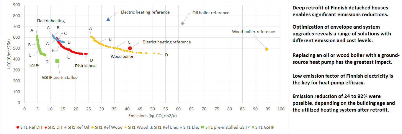
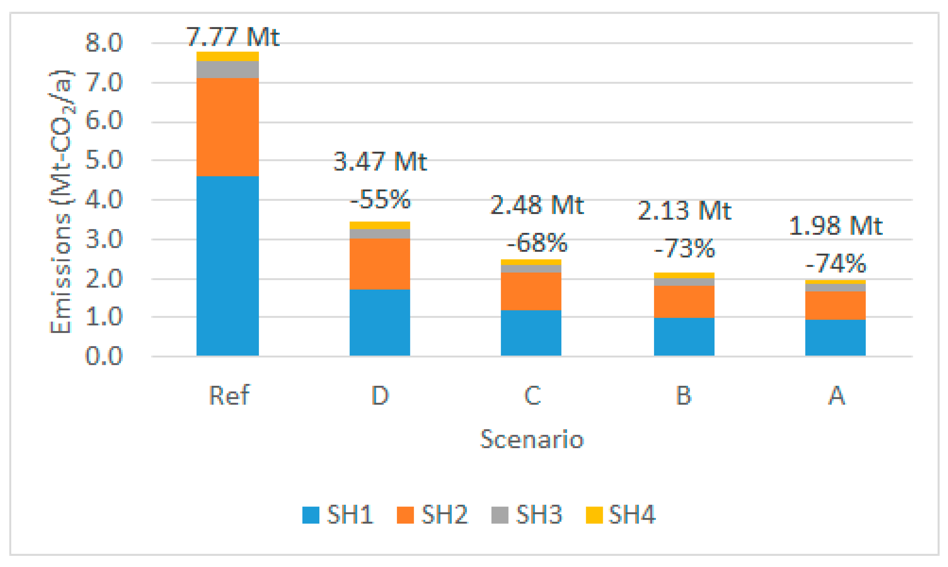
Optimal energy renovation plans were found for Finnish detached houses of four different ages. Cost-effective renovations were possible for every type, reducing CO₂ emissions significantly. The obtained emission reductions were 41% to 92% for the oldest building SH1 and 24% to 85% for the newest building SH4, depending on the selected heating system and investment level. For the whole building stock of detached houses, a 55% emission reduction was possible cost-effectively and a 74% reduction with the highest cost non-economical investments.

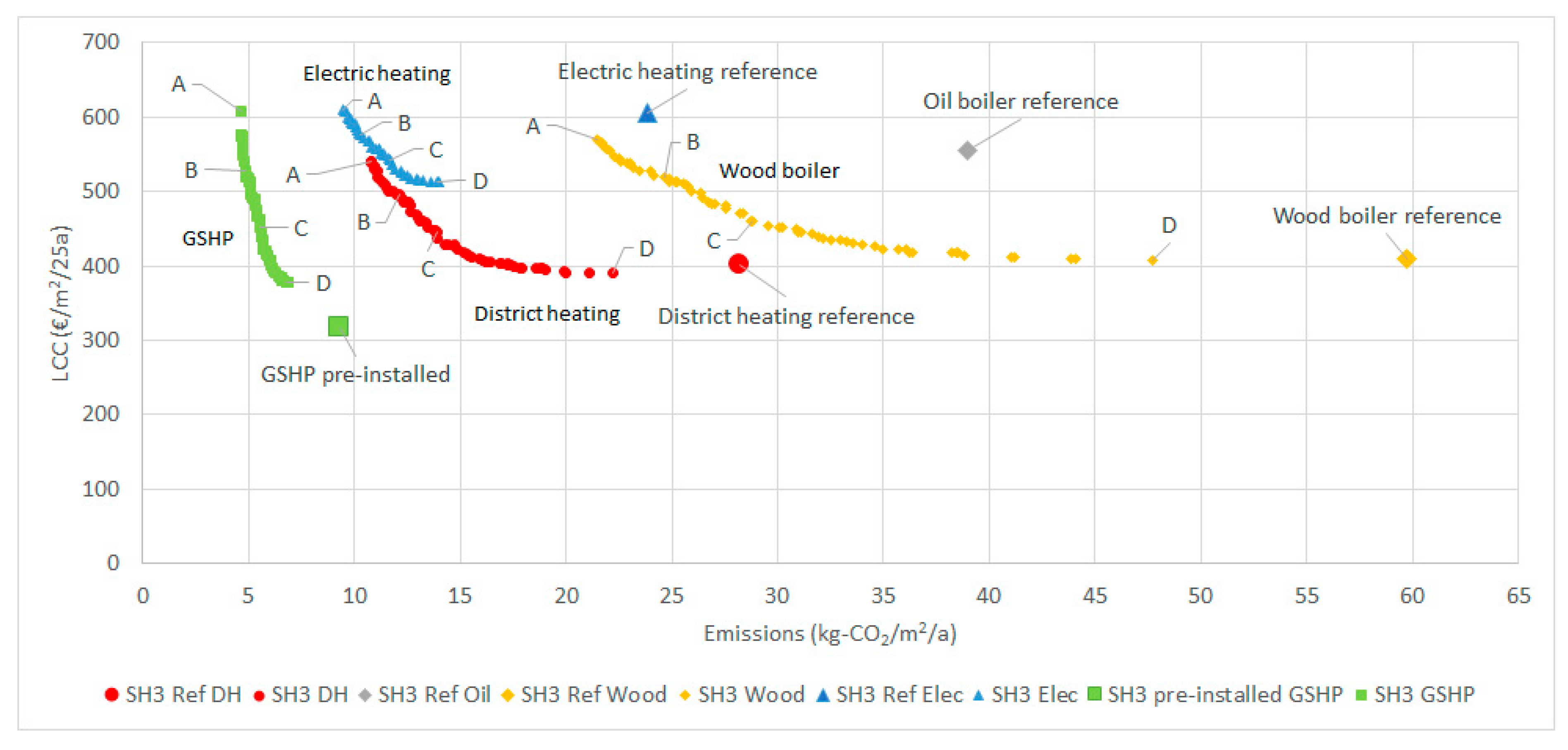
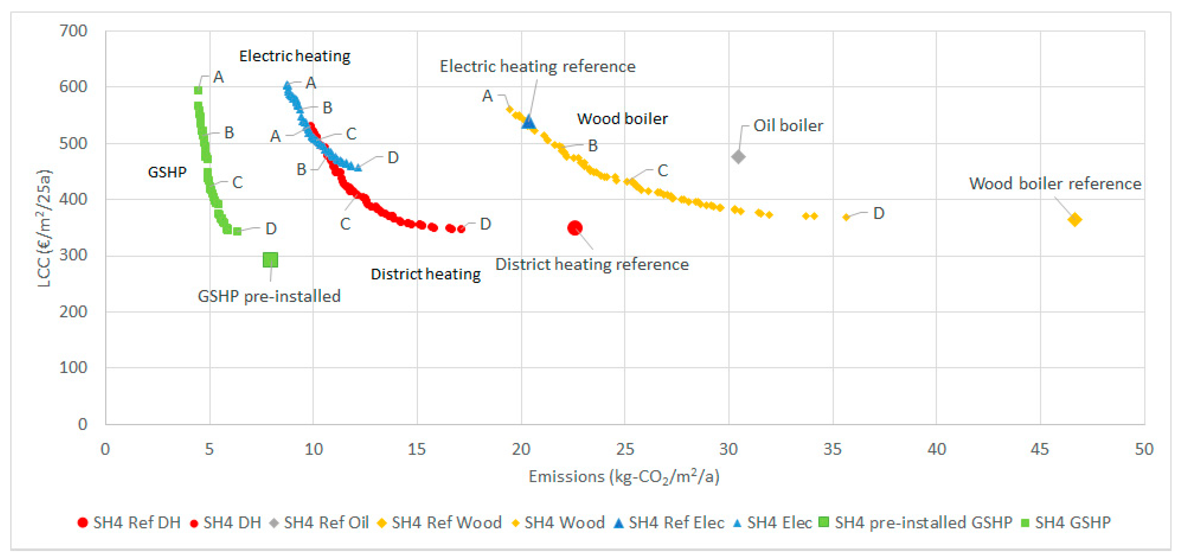
The heating energy source had a big influence on the emissions of the buildings. Electricity has a low emission factor, which made even direct electric heating an option for low emission heating. The main heating systems can be ranked in order from the lowest to highest emissions: ground-source heat pump, direct electric heating, district heating, wood boiler. The final emission ranges for the optimally renovated cases for all building age classes together were 10 to 24 kg-CO₂/m²/a for district heating, 19 to 52 kg-CO₂/m²/a for wood boiler, 9 to 15 kg-CO₂/m²/a for electric heating, and 4 to 8 kg-CO₂/m²/a for the ground-source heat pump.

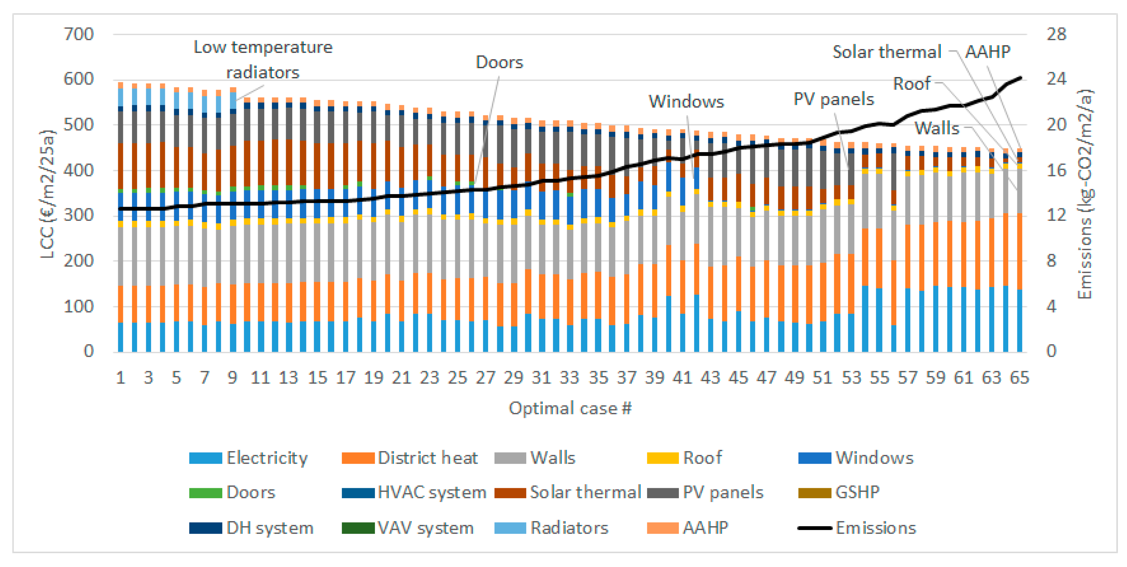
Improving the building envelope was also an effective way to reduce emissions. While, in some cases, additional external wall insulation was not always included in the cheapest solutions, it was still included in a great majority of the optimally retrofitted cases. The newer the building was, the less likely the installation of lower U-value windows. Solar thermal capacity was low or zero for the lowest cost quarter of solutions, but always maximized for the cases with the most ambitious emission reductions. Solar electricity was used in the majority of optimal cases: for all electrically heated cases but not for the lowest cost cases with other heating systems. An air-to-air heat pump was added as auxiliary heating in all optimal solutions.

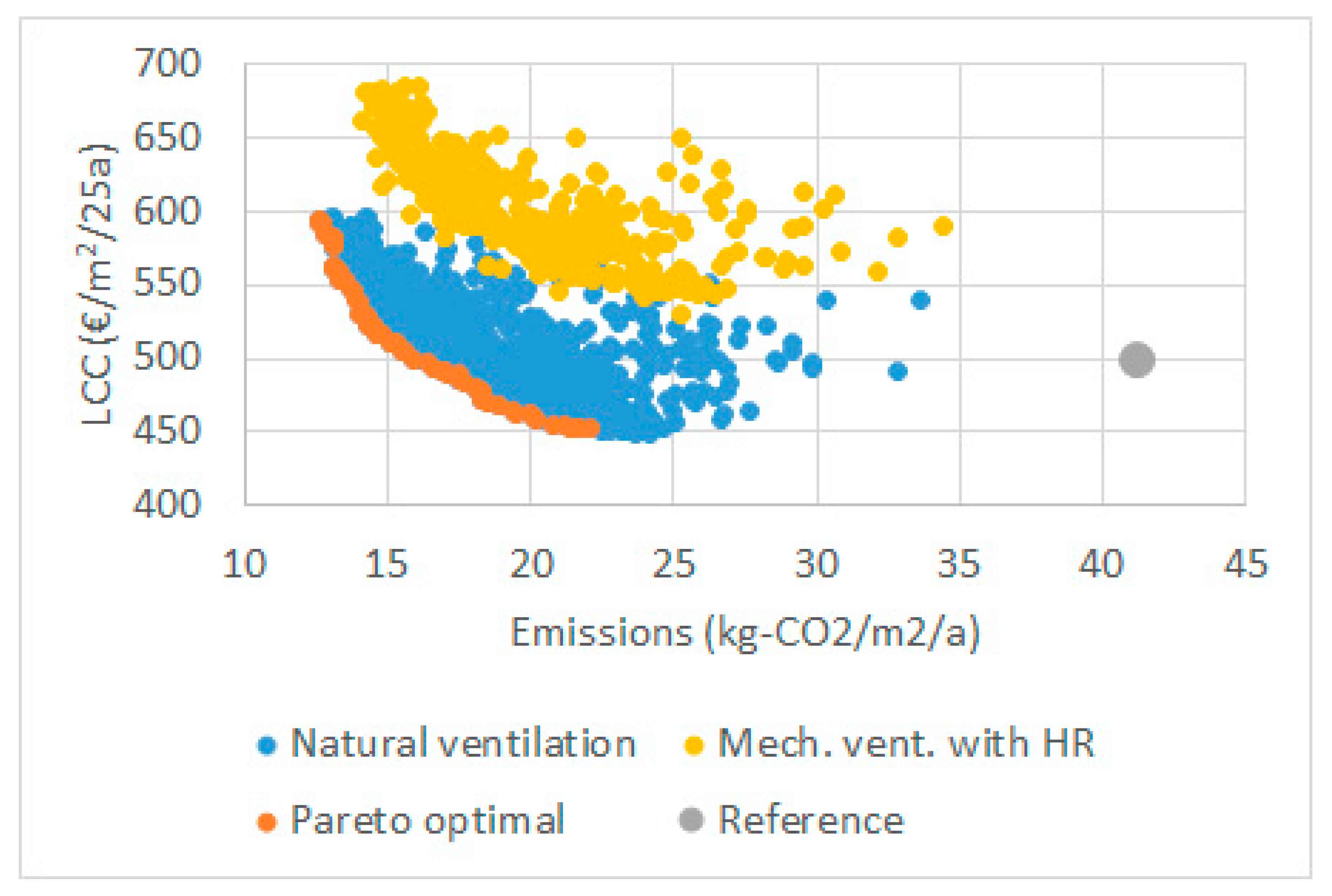
In this optimization study, replacing natural or mechanical exhaust ventilation by mechanical supply and an exhaust ventilation system was not a cost-effective solution in most of the cases because the monetary value of better indoor air quality achieved with a balanced ventilation system was not taken into account. However, in the buildings that already had such ventilation systems (SH3 and SH4) it was beneficial to both install a new AHU with a better heat recovery efficiency and install demand-based ventilation to reduce the heating of unoccupied houses. Installation of a mechanical supply and exhaust ventilation system was cost-effective in the oldest building (SH1) with direct electric heating, due to the very high energy expense.

Cost-effective energy retrofitting was found to be possible in detached houses of every age. For district heating, local boiler and electric heating retrofit solutions with lower LCC compared to the reference cases were found. The GSHP was by default so effective that additional improvements may not be necessary. Replacing boilers by heat pumps had the biggest emission impact. However, these solutions rely on the availability of low emissions electricity. A more detailed study must be done on the building stock to understand how fast the renovations can be done and to estimate how much clean electricity is actually available for use in newly electrified buildings.

References

1. European Commission. EU Climate Action—2050 Long-Term Strategy. 2016. Available online: https://ec.europa.eu/clima/policies/strategies/2050_en (accessed on 3 February 2019).
2. European Parliament. Directive (EU) 2018/844 of the European Parliament and of the Council amending Directive 2010/31/EU on the energy performance of buildings and Directive 2012/27/EU on the energy efficiency. Off. J. Eur. Union 2018, L 156, 75–91. [Google Scholar]
3. Ministry of the Environment. 4/13 Asetus rakennuksen energiatehokkuuden parantamisesta korjaus—ja muutostöissä (4/13 decree on improving energy performance in renovations). Available online: http://www.ym.fi/download/noname/%7B924394EF-BED0-42F2-9AD2-5BE3036A6EAD%7D/31396 (accessed on 7 January 2019).
4. Statistics Finland. Number of Buildings by Intended Use and Year of Construction on 31 December 2015; Statistics Finland: Helsinki, Finland, 2016. [Google Scholar]
5. Ekström, T.; Blomsterberg, Å. Renovation of Swedish Single-family Houses to Passive House Standard – Analyses of Energy Savings Potential. Energy Procedia 2016, 96, 134–145. [Google Scholar] [CrossRef]
6. Taillandier, F.; Mora, L.; Breysse, D. Decision support to choose renovation actions in order to reduce house energy consumption—An applied approach. Build. Environ. 2016, 109, 121–134. [Google Scholar] [CrossRef]
7. Dermentzis, G.; Fabian, O.; Marcus, G.; Toni, C.; Dietmar, S.; Wolfgang, F.; Chiara, D.; Roberto, F.; Chris, B. A comprehensive evaluation of a monthly-based energy auditing tool through dynamic simulations, and monitoring in a renovation case study. Energy Build. 2019, 183, 713–726. [Google Scholar] [CrossRef]
8. Thermal Energy System Specialists, LLC TRNSYS: Transient System Simulation Tool. 2019. Available online: http://www.trnsys.com/ (accessed on 12 September 2019).
9. Hamburg, A.; Kalamees, T. How well are energy performance objectives being achieved in renovated apartment buildings in Estonia? Energy Build. 2019, 199, 332–341. [Google Scholar] [CrossRef]
10. Henning, H.-M.; Palzer, A. A comprehensive model for the German electricity and heat sector in a future energy system with a dominant contribution from renewable energy technologies—Part I: Methodology. Renew. Sustain. Energy Rev. 2014, 30, 1003–1018. [Google Scholar] [CrossRef]
11. Palzer, A.; Henning, H.-M. A comprehensive model for the German electricity and heat sector in a future energy system with a dominant contribution from renewable energy technologies—Part II: Results. Renew. Sustain. Energy Rev. 2014, 30, 1019–1034. [Google Scholar] [CrossRef]
12. Niemelä, T.; Kosonen, R.; Jokisalo, J. Cost-effectiveness of energy performance renovation measures in Finnish brick apartment buildings. Energy Build. 2017, 137, 60–75. [Google Scholar] [CrossRef]
13. Hirvonen, J.; Jokisalo, J.; Heljo, J.; Kosonen, R. Towards the EU emissions targets of 2050: Optimal energy renovation measures of Finnish apartment buildings. Int. J. Sustain Energy 2018, 38, 649–672. [Google Scholar] [CrossRef]
14. Ko, M.J.; Kim, Y.S.; Chung, M.H.; Jeon, H.C. Multi-objective optimization design for a hybrid energy system using the genetic algorithm. Energies 2015, 8, 2924–2949. [Google Scholar] [CrossRef]
15. Tokarik, M.S.; Richman, R.C. Life cycle cost optimization of passive energy efficiency improvements in a Toronto house. Energy Build. 2016, 118, 160–169. [Google Scholar] [CrossRef]
16. Fan, Y.; Xia, X. A multi-objective optimization model for energy-efficiency building envelope retrofitting plan with rooftop PV system installation and maintenance. Appl. Energy 2017, 189, 327–335. [Google Scholar] [CrossRef]
17. Eskander, M.M.; Sandoval-Reyes, M.; Silva, C.A.; Vieira, S.M.; Sousa, J.M.C. Assessment of energy efficiency measures using multi-objective optimization in Portuguese households. Sustain. Cities Soc. 2017, 35, 764–773. [Google Scholar] [CrossRef]
18. Ren, G.; Heo, Y. Sunikka-Blank Investigating an adequate level of modelling for retrofit decision-making: A case study of a British semi-detached house. J. Build. Eng. 2019, 26, 100837. [Google Scholar] [CrossRef]
19. Alev, Ü.; Allikmaa, A.; Kalamees, T. Potential for Finance and Energy Savings of Detached Houses in Estonia. Energy Procedia 2015, 78, 907–912. [Google Scholar] [CrossRef]
20. Leinartas, H.A.; Stephens, B. Optimizing Whole House Deep Energy Retrofit Packages: A Case Study of Existing Chicago-Area Homes. Buildings 2015, 5, 323–353. [Google Scholar] [CrossRef]
21. Ekström, T.; Bernardo, R.; Blomsterberg, Å. Cost-effective passive house renovation packages for Swedish single-family houses from the 1960s and 1970s. Energy Build. 2018, 161, 89–102. [Google Scholar] [CrossRef]
22. Asaee, S.R.; Ugursal, V.I.; Beausoleil-Morrison, I. Techno-economic feasibility evaluation of air to water heat pump retrofit in the Canadian housing stock. Appl. Therm. Eng. 2017, 111, 936–949. [Google Scholar] [CrossRef]
23. Asaee, S.R.; Ugursal, V.I.; Beausoleil-Morrison, I. Techno-economic assessment of solar assisted heat pump system retrofit in the Canadian housing stock. Appl. Energy 2017, 190, 439–452. [Google Scholar] [CrossRef]
24. Bjørneboe, M.G.; Svendsen, S.; Heller, A. Evaluation of the renovation of a Danish single-family house based on measurements. Energy Build. 2017, 150, 189–199. [Google Scholar] [CrossRef]
25. Psomas, T.; Heiselberg, P.; Duer, K.; Bjørn, E. Overheating risk barriers to energy renovations of single family houses: Multicriteria analysis and assessment. Energy Build. 2016, 117, 138–148. [Google Scholar] [CrossRef]
26. Beccali, M.; Cellura, M.; Fontana, M.; Longo, S.; Mistretta, M. Energy retrofit of a single-family house: Life cycle net energy saving and environmental benefits. Renew. Sustain. Energy Rev. 2013, 27, 283–293. [Google Scholar] [CrossRef]
27. Azizi, S.; Nair, G.; Olofsson, T. Analysing the house-owners’ perceptions on benefits and barriers of energy renovation in Swedish single-family houses. Energy Build. 2019, 198, 187–196. [Google Scholar] [CrossRef]
28. Bjørneboe, M.G.; Svendsen, S.; Heller, A. Initiatives for the energy renovation of single-family houses in Denmark evaluated on the basis of barriers and motivators. Energy Build. 2018, 167, 347–358. [Google Scholar] [CrossRef]
29. Pornianowski, M.; Antonov, Y.I.; Heiselberg, P. Development of energy renovation packages for the Danish residential sector. Energy Procedia 2019, 158, 2847–2852. [Google Scholar] [CrossRef]
30. Mortensen, A.; Heiselberg, P.; Knudstrup, M. Economy controls energy retrofits of Danish single-family houses. Comfort, indoor environment and architecture increase the budget. Energy Build 2014, 72, 465–475. [Google Scholar] [CrossRef]
31. EQUA Simulation AB, IDA ICE—Simulation Software. 2019. Available online: https://www.equa.se/en/ida-ice (accessed on 8 August 2019).
32. EQUA Simulation AB. Validation of IDA indoor climate and energy 4.0 with respect to CEN standards EN 15255-2007 and EN 15265-2007; EQUA Simulation AB: Solna, Sweden, May 2010. [Google Scholar]
33. Loutzenhiser, P.; Manz, H.; Maxwell, G. Empirical validations of shading/daylighting/load interactions in building energy simulation tools. IEA Int. Energy Agency 2007, 7, 1426–1431. [Google Scholar]
34. Kalamees, T.; Jylhä, K.; Tietäväinen, H.; Jokisalo, J.; Ilomets, S.; Hyvönen, R.; Saku, S. Development of weighting factors for climate variables for selecting the energy reference year according to the EN ISO 15927-4 standard. Energy Build. 2012, 47, 53–60. [Google Scholar] [CrossRef]
35. Finnish Meteorological Institute. Test Reference Years for Energy Calculations; Finnish Meteorological Institute: Helsinki, Finland, 19 November 2018. (In Finnish) [Google Scholar]
36. Palonen, M.; Hamdy, M.; Hasan, A. MOBO a new software for multi-objective building performance optimization. In Proceedings of the 13th Conference of International Building Performance Simulation Association, Chambéry, France, 2013. [Google Scholar]
37. Ministry of the Environment. Directive on building energy certificates, Attachment 1. Available online: https://www.finlex.fi/data/sdliite/liite/6822.pdf (accessed on 12 December 2019). (In Finnish).
38. Statistics Finland. Email Query about Building Heating System Statistics; Statistics Finland: Helsinki, Finland, 2017. [Google Scholar]
39. Haakana, M. Ympäristöministeriön Asetus Rakennuksen Energiatodistuksesta; Finlex: Helsinki, Finland, 2017. [Google Scholar]
40. Laitinen, A. Air-to-Air Heat Pump Energy Consumption Effect in Detached Houses; VTT: Finland, Espoo, 2016. (In Finnish) [Google Scholar]
41. NIBE AB. NIBE F1345 Heat Pump Installer Manual; NIBE AB: Sweden, Markaryd, 2017. [Google Scholar]
42. CEN European Committee for Standardization. Standard EN 14511-3:2013. Air Conditioners, Liquid Chilling Packages and Heat Pumps with Electrically Driven Compressors for Space Heating and Cooling. Part 3: Test methods. 2013. Available online: https://www.en-standard.eu/din-en-14511-1-air-conditioners-liquid-chilling-packages-and-heat-pumps-for-space-heating-and-cooling-and-process-chillers-with-electrically-driven-compressors-part-1-terms-and-definitions/ (accessed on 8 January 2019).
43. Koivuniemi, J. Lämpimän käyttöveden mitoitusvirtaama ja lämpötilakriteerit veden mikrobiologisen laadun kannalta kaukolämmitetyissä taloissa [Domestic hot water design flow and temperature criteria as pertains to water microbiological quality in district heated houses, In Finnish]. Mster′s Thesis, Helsinki University of Technology, Espoo, Finland, 2005. [Google Scholar]
44. Ministry of the Environment. Ympäristöministeriön asetus uuden rakennuksen energiatehokkuudesta (1010/2017) (Decree of the Ministry of the Environment on the energy performance of the new building (1010/2017); 2018. Available online: https://www.finlex.fi/fi/laki/alkup/2017/20171010 (accessed on 14 December 2018). (In Finnish).
45. Degefa, M.Z. Project Report of SGEM Task 6.11: Spatial load analysis; Aalto University School of Electrical Engineering: Espoo, Finland, 2012. [Google Scholar]
46. Ministry of the Environment. D3—Rakennusten energiatehokkuus; Ministry of the Environment: Helsinki, Finland, 2012. (In Finnish) [Google Scholar]
47. Finnish Energy. Emission factors of Finnish Electricity, Email Contact; Finnish Energy: Helsinki, Finland, 2017. [Google Scholar]
48. Motiva Oy, CO2 emission factors in Finland. 2019. Available online: https://www.motiva.fi/ratkaisut/energiankaytto_suomessa/co2-laskentaohje_energiankulutuksen_hiilidioksidipaastojen_laskentaan/co2-paastokertoimet (accessed on 15 January 2019). (In Finnish).
49. Statistics Finland. Fuel Classification 2019; Statistics Finland: Helsinki, Finland, 2019. (In Finnish) [Google Scholar]
50. Finnish Energy, 2018. Available online: https://energia.fi/en (accessed on 8 Augest 2019).
51. Fortum, District Heating Price [In Finnish]. 2019. Available online: https://www.fortum.fi/kotiasiakkaille/lammitys/kaukolampo/kaukolammon-hinnat-pientaloille (accessed on 1 January 2019).
52. Vapo Oy, Wood Fuel Price. 2019. Available online: https://kauppa.vapo.fi/tuotteet/500-kg-pellettisakki/ (accessed on 15 April 2019).
53. Lämpöpuisto Oy, Heating Oil Price [In Finnish]. 2019. Available online: https://www.lampopuisto.fi/fi/yksityisille/lammitysoljyn-hinta (accessed on 16 April 2019).
54. Nord Pool, Historical Electricity Market Data. 2018. Available online: https://www.nordpoolgroup.com/historical-market-data/ (accessed on 14 January 2019).
55. Caruna Oy, Electricity Distribution Pricing. 2019. Available online: https://www.caruna.fi/en/our-services/products-and-rates/electricity-distribution-rates (accessed on 13 February 2019).
56. Lindberg, R.; Kivimäki, C.; Sahlstedt, S. Korjausrakentamisen kustannuksia 2019 [Cost of building renovation, in Finnish]; Rakennustieto Oy: Helsinki, Finland, 2019. [Google Scholar]
57. Taloon.com, Taloon.com web store. 2019. Available online: https://www.taloon.com (accessed on 3 December 2019).
58. Motiva Oy, Solar electric system prices. Aurinkosähköä kotiin, 2019. Available online: https://aurinkosahkoakotiin.fi/tarjoukset/ (accessed on 12 August 2019). (In Finnish).
59. Deb, K.; Pratap, A.; Agarwal, S.; Meayarivan, T. A fast and elitist multiobjective genetic algorithm: NSGA-II. IEEE Trans. Evol. Comput. 2002, 6, 182–197. [Google Scholar] [CrossRef]
60. Business Insider, European Emission Allowance prices. markets.businessinsider.com. 2019. Available online: https://markets.businessinsider.com/commodities/co2-european-emission-allowances (accessed on 12 September 2019).
61. Paiho, S.; Reda, F. Towards next generation district heating in Finland. Renew. Sustain. Energy Rev. 2016, 65, 915–924. [Google Scholar] [CrossRef]
62. Värri, K.; Syri, S. The possible role of modular nuclear reactors in district heating: Case Helsinki region. Energies 2019, 12, 2195. [Google Scholar] [CrossRef]
63. Partanen, R. Nuclear District Heating in Finland—The Demand, Supply and Emissions Reduction Potential of Heating Finland with Small Nuclear Reactors. Think Atom, February. 2019. Available online: https://thinkatomnet.files.wordpress.com/2019/04/nuclear-district-heating-in-finland_1-2_web.pdf (accessed on 7 June 2019).
64. Persson, U.; Werner, S. Quantifying the Heating and Cooling Demand in Europe; D 2.2; Halmstad University: Halmstad, Sweden, 2015. [Google Scholar]
65. Hrovatin, N.; Zorić, J. Determinants of energy-efficient home retrofits in Slovenia: The role of information sources. Energy Build. 2018, 180, 42–50. [Google Scholar] [CrossRef]
66. Hirvonen, J.; Rehman, H.; Sirén, K. Techno-economic optimization and analysis of a high latitude solar district heating system with seasonal storage, considering different community sizes. Sol. Energy 2018, 162, 472–488. [Google Scholar] [CrossRef] [Green Version]
67. Hirvonen, J.; Sirén, K. A novel fully electrified solar heating system with a high renewable fraction—Optimal designs for a high latitude community. Renew. Energy 2018, 127, 298–309. [Google Scholar] [CrossRef]
Figure 1. The optimization process that combines the three tools.
Energies 12 04395 g001
Figure 2. Distribution of built floor area in single-family houses over different construction periods.
Energies 12 04395 g002
Figure 3. Heating systems in single-family houses. [38].
Energies 12 04395 g003
Figure 4. Retrofit paths for buildings with different heating systems.
Energies 12 04395 g004
Figure 5. Specific heating demand in the reference buildings.
Energies 12 04395 g005
Figure 6. Results from the optimization of SH1 with district heating. Mechanical ventilation cases are shown in a separate cluster due to their higher investment costs. Mechanical supply and exhaust ventilation improve indoor air quality, which is not considered in the optimization.
Energies 12 04395 g006
Figure 7. Breakdown of life cycle cost for SH1 with district heating.
Energies 12 04395 g007
Figure 8. Reference cases and optimal results for the oldest single-family house SH1 with different heating systems. The cost and emissions of the reference cases are shown with large individual symbols. The corresponding optimal results are shown as Pareto fronts with the same color. Four individual solutions were chosen from each Pareto front, identified with the letters A to D. A is the most expensive solution, and D the least cost solution, with B and C equally distributed between them.
Energies 12 04395 g008
Figure 9. Reference cases and optimal results of retrofitting for the single-family house SH2 with different heating systems.
Energies 12 04395 g009
Figure 10. Reference cases and optimal results for the single-family house SH3 with different heating systems.
Energies 12 04395 g010
Figure 11. Reference cases and optimal results for the single-family house SH4 with different heating systems.
Energies 12 04395 g011
Figure 12. Assumed distribution of heating systems in the optimized scenarios.
Energies 12 04395 g012
Figure 13. Absolute carbon emissions of the whole detached house building stock in Finland in the reference and optimized scenarios. The numbers show the remaining total CO2 emissions and the relative reduction compared to the reference case.
Energies 12 04395 g013