Article

Impact of Flexible AC Transmission System Devices on Automatic Generation Control with a Metaheuristic Based Fuzzy PID Controller

by
Ramana Pilla
1,
Ahmad Taher Azar
2,3,* and
Tulasichandra Sekhar Gorripotu
4,*
1
Department of EEE, GMR Institute of Technology, Rajam, Srikakulam, Andhra Pradesh 532127, India
2
Robotics and Internet-of-Things Lab (RIOTU), Prince Sultan University, Riyadh 12435, Saudi Arabia
3
Faculty of Computers and Artificial Intelligence, Benha University, Benha 13511, Egypt
4
Department of EEE, Sri Sivani College of Engineering, Srikakulam, Andhra Pradesh 532410, India
*
Authors to whom correspondence should be addressed.
Energies 2019, 12(21), 4193; https://doi.org/10.3390/en12214193
Submission received: 19 September 2019 / Revised: 25 October 2019 / Accepted: 29 October 2019 / Published: 2 November 2019
(This article belongs to the Section F: Electrical Engineering)

Abstract

:
The present work proposes a teaching–learning-based optimization (TLBO)-tuned fuzzy proportional-integral-derivative (PID) controller of two-area hydro-thermal generating units for automatic generation control (AGC). The proposed system takes into account the physical constraints such as transport delay (TD), generation rate constraint (GRC), and governor dead band (GDB) nonlinearities. Firstly, fuzzy PID controllers were designed for both the areas and their gains were optimized using various minimization objective function criteria. Furthermore, applications of flexible alternating current transmission system (FACTS) devices such as static synchronous series compensator (SSSC), thyristor-controlled series capacitor (TCSC), thyristor-controlled phase shifter (TCPS), and unified power flow controller (UPFC) were investigated by integrating FACTS devices in appropriate locations of the system. The simulation results revealed that the minimum objective values were attained when the UPFC was placed in the system. Lastly, robustness analysis was done to observe the capability of the proposed controller with UPFC by changing system parameters and considering random load disturbances.

1. Introduction

In recent years, the consumption of power increased gradually regardless of power generation. This sudden increase in load creates some imbalances in power system operation such as the frequency and tie-line power deviations. This problem can be avoided by connecting a fast-acting automatic generation control for controlling the power generation between various control areas by holding the frequency as constant [1,2,3,4]. Automatic generation control plays a vital role in large-scale interconnected electrical power units to maintain the frequency and tie-line power as close as possible to the pre-defined values. The speed governing system in the AGC helps to manage the frequency and tie-line power within pre-defined values by varying the mechanical power input to the generators. A healthy power system must supervise the load changes and system disturbances to ensure an acceptable quality of power through the preservation of voltage and frequency within acceptable boundaries [5,6,7,8].
Several researchers focused on the significance of AGC and reported several soft computing techniques for obtaining optimal values of secondary controllers [9,10,11,12,13,14,15,16]. For example, Guha et al. [14] introduced a backtracking search evolutionary algorithm for the load frequency control (LFC) of power systems. Fathy and Kassem [15] initiated an optimal LFC using a tuned adaptive neuro fuzzy inference system with an antlion optimizer. Pradhan and Bhende [16] proposed the online LFC of a power system based on a modification of the Jaya heuristic search algorithm. Khadanga and Kumar [17] executed a PID controller tuned by particle swarm optimization and a gravitational search algorithm for the LFC of a multi-source multi-area system. The performance of the high voltage AC or DC (HVAC/DC) link in the AGC was also presented, along with the ability of the static synchronous series compensator (SSSC) and capacitive energy storage (CES) devices. Guha et al. [18] initiated a differential search algorithm (DSA) for different power systems by considering a proportional-integral-derivative with filter (PIDF) controller, and they also showed its ability through a comparative analysis with other techniques. Chandrakala and Balamurugan [19] developed a combined system of an LFC and automatic voltage regulator (AVR) for a multi-source multi-area system tuned by simulated annealing. Ali and Abd-Elazim [20] proposed a bacterial foraging optimization algorithm to tune the parameters of a PID controller for a nonlinear LFC. Shabani et al. [21] proposed a resistant differential PID control technique tuned by an imperialist competitive algorithm for an LFC to eliminate the effect of disturbance.
In general, AGC is a slow control task; however, classical controllers like PID allow the system to react rapidly while varying its gain values, and its design is effortless. The proportional term helps the system to diminish the rise time, the integral term purges the steady-state error, and the derivative term improves the stability. The fuzzy PID controller has advantages over classical controllers, as its parameters can be tuned without having much knowledge on the system, and it exhibits simpler design properties than gain scheduling controllers [22,23,24,25,26]. In this paper, the teaching–learning-based optimization (TLBO) technique is proposed to produce optimal values, as it does not depend on any specific parameter [27]. Several researchers investigated flexible alternating current transmission system (FACTS) devices participating in power system applications for transient stability improvement [28,29,30]. For improving and speeding up performance in AGC, some FACTS devices are included in the power system model [31,32]. By taking all these issues into consideration, the present paper proposes controlling the AGC of a multi-area power system by using FACTS devices with the inclusion of non-linearities. The main objectives of the present work are as follows:
  • To recommend a teaching–learning-based optimization (TLBO)-based fuzzy PID controller for the AGC problem;
  • To illustrate the superiority of the fuzzy PID controller with non-linearities such as the transport delay (TD), generation rate constraint (GRC), and governor dead band (GDB) for the AGC problem;
  • To demonstrate the performance of various FACTS devices incorporated in the system;
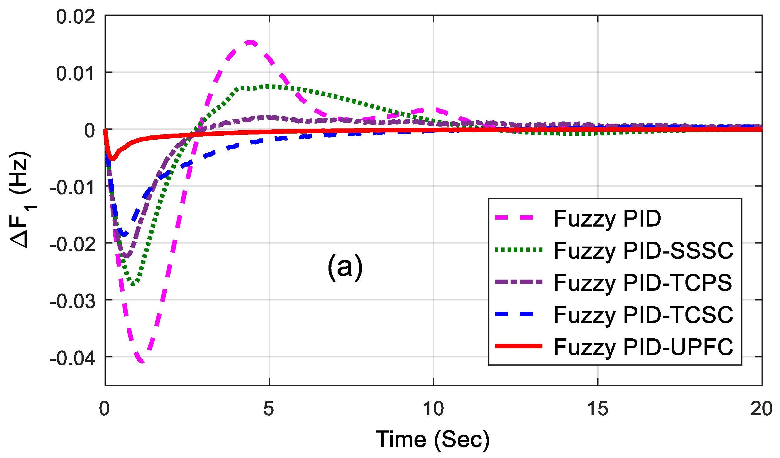
  • To observe the effectiveness of the fuzzy PID plus unified power flow controller (UPFC) device for various disturbances such as step and random step load disturbances.
The rest of the paper is organized as follows: Section 2 shows the methodology of the system model. Section 3 discusses the teaching–learning-based optimization algorithm. Simulation results, along with their analysis, are shown in Section 4. The concluding remarks about the designed controller are presented in Section 5.

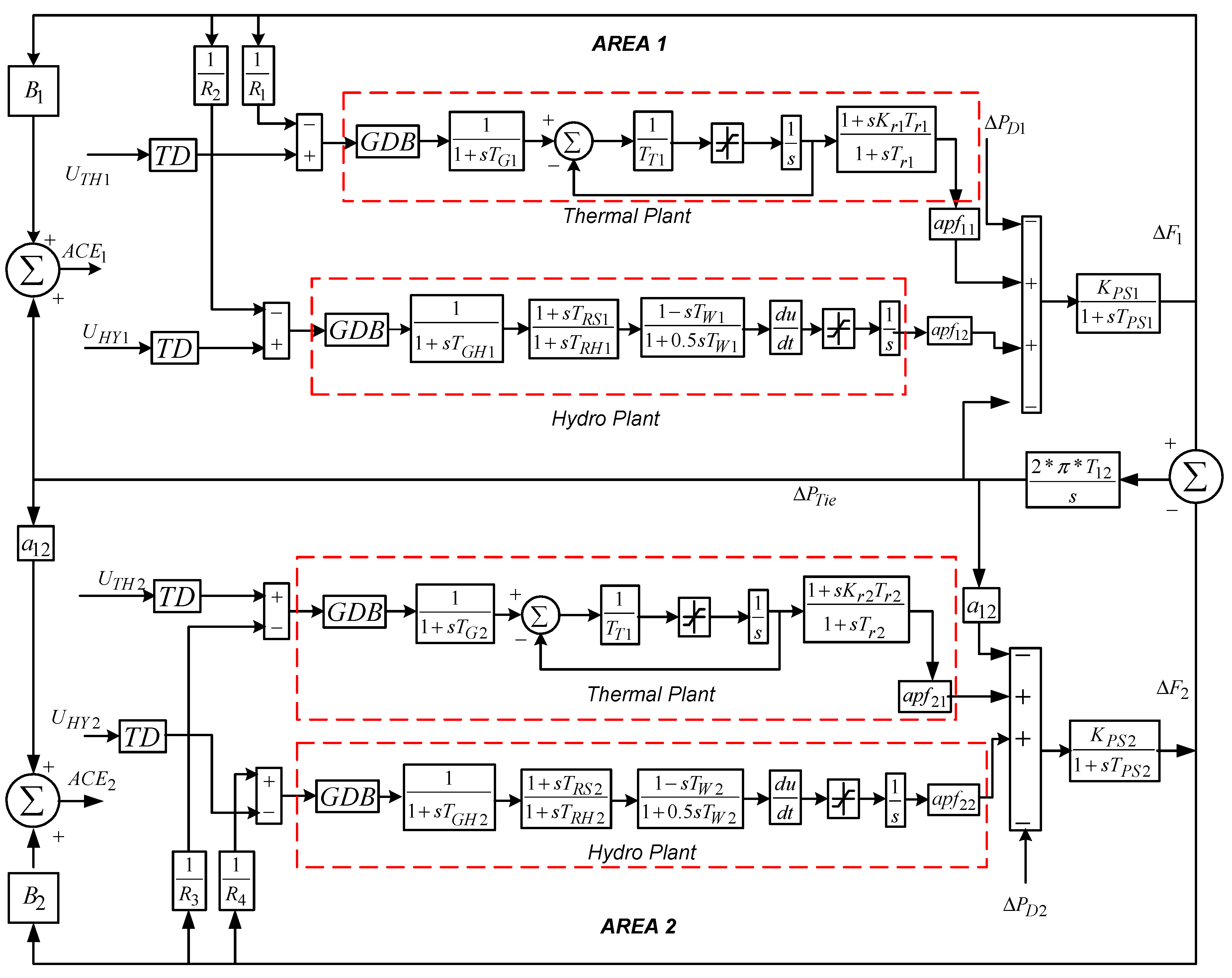
2. Materials and Methods

In this paper, a two-area four-unit hydro and thermal system of equal 2000MW power capacity with 1640MW as nominal loading was examined. The analysis was made in a per unit system by considering 2000MW as a base value. The transfer function models of the thermal and hydro units were designed in MATLAB/SIMULINK (9.1.0.441655, R2016b version, Mathematical computing software, Natick, MA, USA) environment, and their related diagram is shown in Figure 1. The corresponding parameter values are specified in Appendix A. The considered power system shown in Figure 1 includes all the appropriate non-linearities such as GRC, GDB, and TD. The contribution of the different generating units contributing to the AGC problem are also represented by participation factors. In present work, the hydro and thermal units contributed equally with a participation factor of 0.5. To have a realistic study, some non-linearities were considered. The thermal units in both areas were incorporated with a reheat turbine, a GDB of 0.05%, and a GRC of 3%. Similarly, hydro units were incorporated with a GDB of 0.02% and a GRC of 6%. A transport delay of 50 ms was also introduced for each generating unit, which considered the delay process of the system’s components.

Control Structure

Linear controllers such as integral (I), proportional-integral (PI), proportional-derivative (PD), and proportional-integral-derivative PID controllers were used to get the required transient and steady-state performance in various power electronics and power system applications to attain specified control objectives. However, linear controllers are not suitable for systems having higher order, with time delay and non-linearities. Fuzzy logic controllers (FLC) are non-linear controllers, which work well in closed-loop control systems; however, these controllers require fine-tuning in their design and implementation. Many researchers established that FLCs improve the closed-loop performance of classical controllers by updating the controller parameters online to handle the changes in the operating point [33,34,35,36,37]. However, the main limitation of the FLC is the lack of a systematic design process, and improper tuning of parameters may lead to the divergence of system stability. The tuning of FLC with rule-based membership functions (MFs) is complicated and, hence, may not be efficient. Gain tuning must be implemented, as it is the most familiar way of tuning the FLC to enhance the performance [33]. Therefore, rule-based standard MFs can be used for various applications, and scaling factors can be tuned for optimum fuzzy PID control [33]. Taking all these considerations into account, the fuzzy PID controller was chosen here to solve the AGC problem, as shown in Figure 2. The fuzzy controller uses the error ( e ) and derivative of error ( e ˙ ) as input signals. In the present study, the input signal was the area control error of the power system. Here, K1 and K2 were the input scaling factors of the FLC. The FLC output was multiplied with KP, KI, and KD and then summed to give the total controller output. The outputs of the fuzzy controllers U T H i and U H Y i were the control inputs of the power system.
The fuzziness of the FLC is characterized by MFs having different shapes such as triangular, bell, trapezoidal, sigmoid, gaussian, and piecewise linear. Out of these, bell, triangular, and trapezoidal MFs are preferred for real-time applications as they can be represented easily, need nominal memory storage, and can be manipulated efficiently through a fuzzy interface engine. From the literature, triangular MFs were extensively implemented in controller design, as the parametric practical depiction of these MFs is economical when compared to other MFs. Therefore, triangular MFs were considered in the present study. Moreover, an identical representation of MFs is preferred for having better computational effectiveness and superior memory usage [36]. Thus, similar MFs were selected for error, error derivative, and FLC output. The structure of the MFs (Mamdani type) is shown in Figure 3, which was considered for both the inputs and outputs.
While evaluating the performance of any system through an optimization technique, an objective function must be defined based on the preferred constraints. Objective functions such as the integral of time-weighted absolute error (ITAE), integral of squared error (ISE), integral of time-weighted squared error (ITSE), and integral of absolute error (IAE) were used for the present study from the literature [21]. The ITAE criterion provides superior performance in terms of settling time and peak overshoot when compared to IAE and ISE. Hence, ITAEwas considered as the objective function in the present study, which allowed obtaining the optimal controller parameters of the fuzzy PID controller along with its scaling factors. However, the other objective functions IAE, ISE, and ITSE were also evaluated for the purpose of analysis. The expressions for the objective functions are provided in Equations (1)–(4).
J 1 = I S E = 0 t s i m ( | Δ F 1 | + | Δ F 2 | + | Δ P T i e | ) 2 d t .
J 2 = I A E = 0 t s i m ( | Δ F 1 | + | Δ F 2 | + | Δ P T i e | ) . d t .
J 3 = I T S E = 0 t s i m ( | Δ F 1 | + | Δ F 2 | + | Δ P T i e | ) 2 . t . d t .
J 4 = I A E = 0 t s i m ( | Δ F 1 | + | Δ F 2 | + | Δ P T i e | ) . t . d t .

3. Teaching–Learning-Based Optimization (TLBO) Algorithm

The TLBO algorithm attracted the attention of several researchers, it was used for various engineering applications following its initiation in 2011 [27]. This algorithm does not utilize any detailed parameters like some other population-based or metaheuristics algorithms. It results in a constant convergence outcome and has the capacity to produce a high-convergence solution in a minimum time span. Mostly, the working principle of the TLBO algorithm depends on the student’s nature and the influence of the training of the teacher in a classroom atmosphere. The teacher phase and learner phase are the two major phases of TLBO, where students (learners) acquire knowledge from the teacher in the teacher phase, while students acquire knowledge through interaction between learners (students) in the learner phase. The flowchart of the TLBO algorithm is shown in Figure 4. The various actions concerned in the TLBO algorithm are described as below [27].

3.1. Intilization

In this phase, the initial population of range NPD is arbitrarily produced, where NP is the size of the population (number of learners), and D is the dimension of the problem (number of offered subjects). The ith column of the initial population signifies the marks secured by different learners in the ith subject.
The initial population is given as follows:
X = [ x 1 , 1 x 1 , 2 .... x 1 , D x 2 , 1 x 2 , 2 .... x 2 , D . . . . . . x N P , 1 x N P , 2 .... x N P , D ] .

3.2. Teacher Phase

In this phase, every teacher evaluates the mean outcome of a class in the study allocated to them. The teacher instructs the supposedly apt learners, whereby the best solution is recognized and allocated by the teacher. Marks acquired by various students for each subject can be calculated as follows:
M d = [ m 1 , m 2 , ..... , m D ] .
The variation among the mean outcome in a specific subject and the result of the corresponding teacher are given by
M d i f f = r a n d ( 0 , 1 ) [ X b e s t T F M d ] ,
where r a n d ( 0 , 1 ) is a random number between 0 and 1, and T F is the teaching feature; its value is considered as either 1 or 2 and determined randomly using Equation (8).
T F = r o u n d   [ 1 + r a n d ( 0 , 1 ) ] .
The active population is simplified using Equation (9).
X n e w = X + M d i f f .
If f ( X n e w ) < f ( X ) , then elements of X n e w are accepted.

3.3. Learner Phase

In this phase, a learner chooses another learner randomly and aims to enhance their intelligence through communication. A learner develops their ability via communication if the other learner has more knowledge than them. The process of learning can be described as follows:
Select two learners X i and X j randomly such that i j as follows:
X n e w = X i + r a n d ( 0 , 1 ) ( X i X j ) ,    if    f ( X i ) < f ( X j ) ,
else
X n e w = X i + r a n d ( 0 , 1 ) ( X j X i )
Admit X n e w if it produces a better result.

4. Results and Discussion
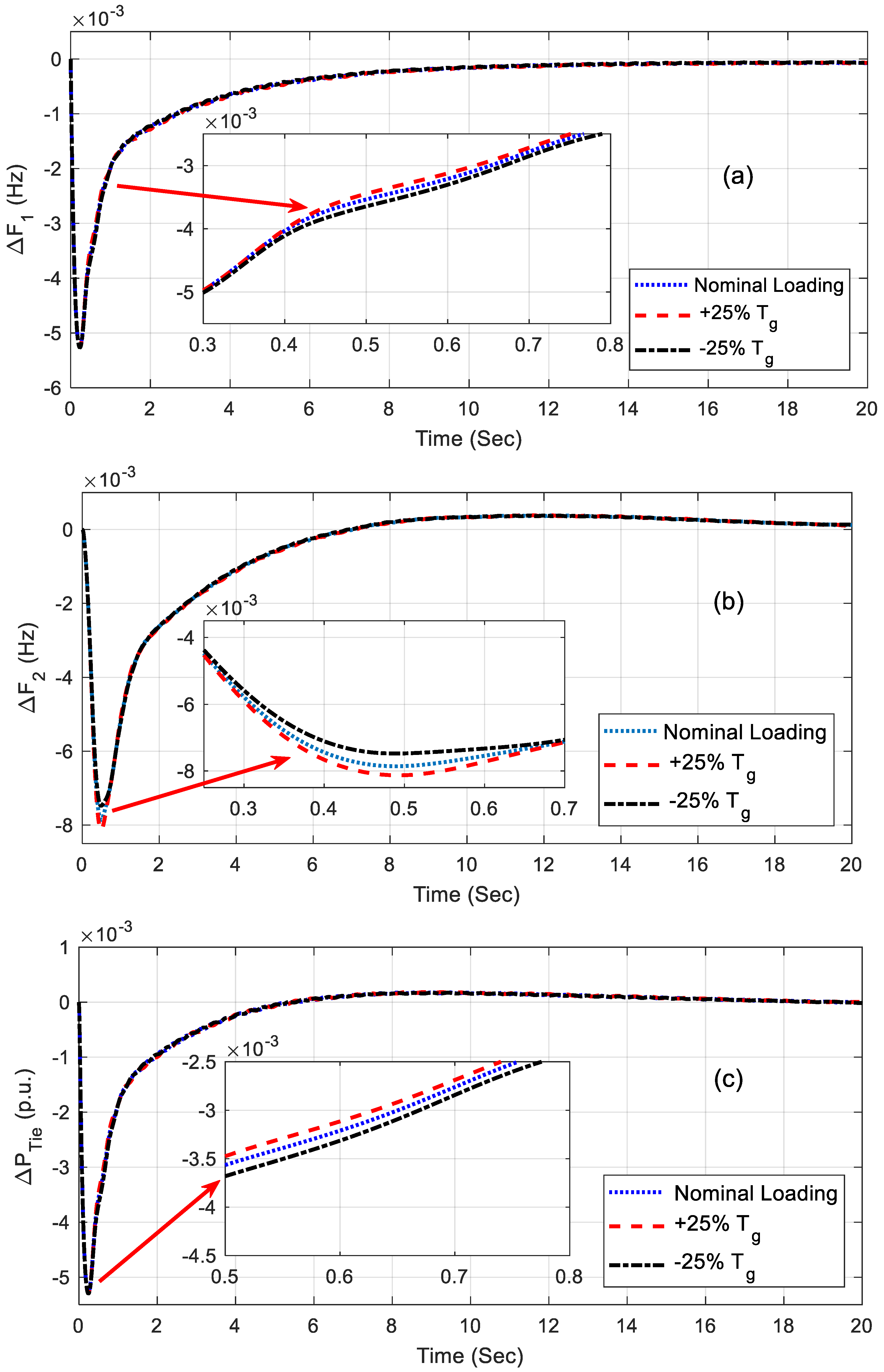
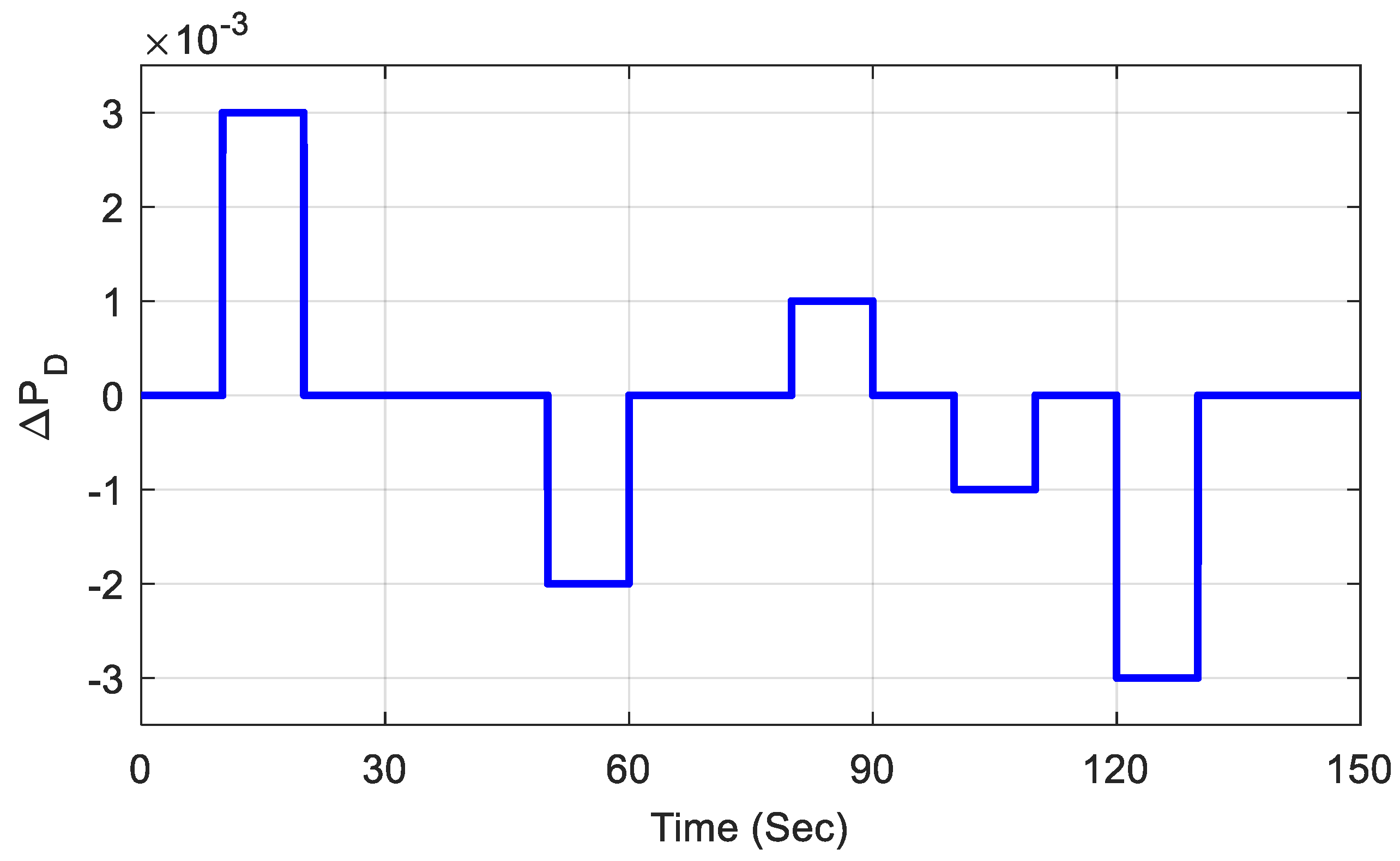
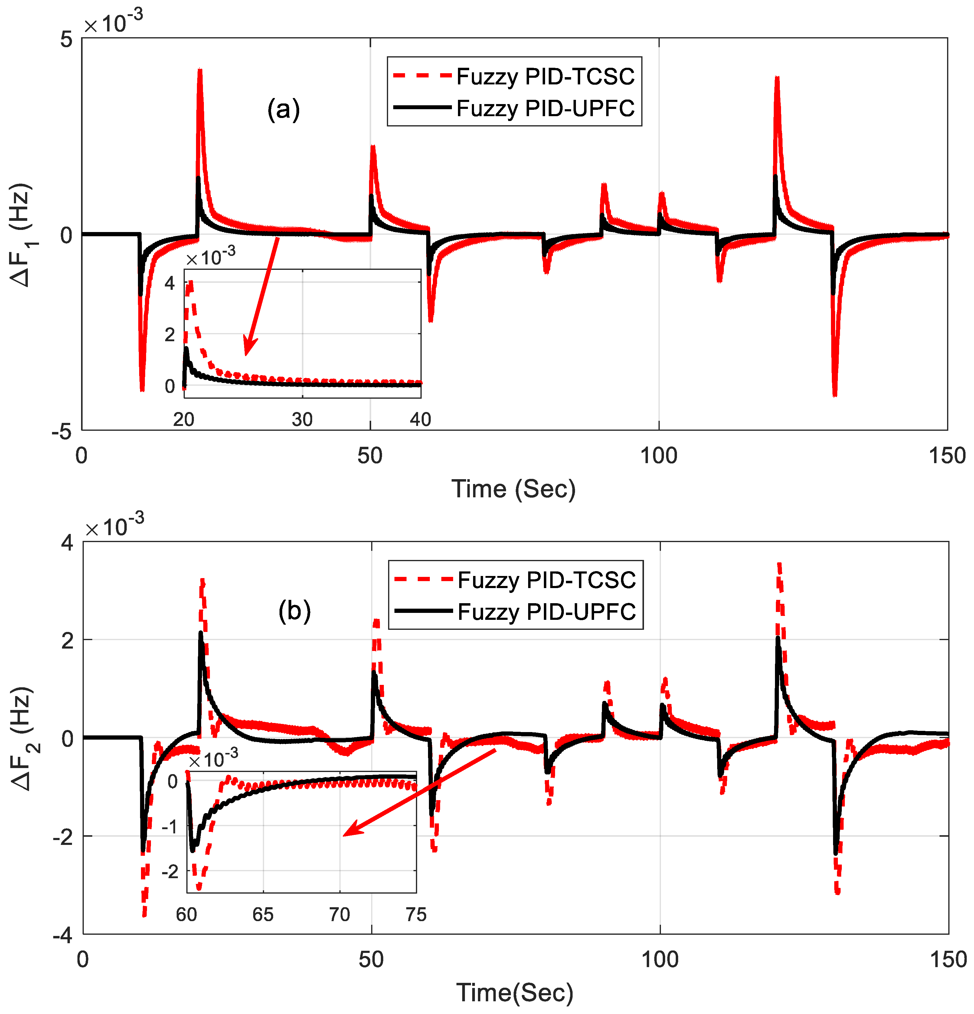
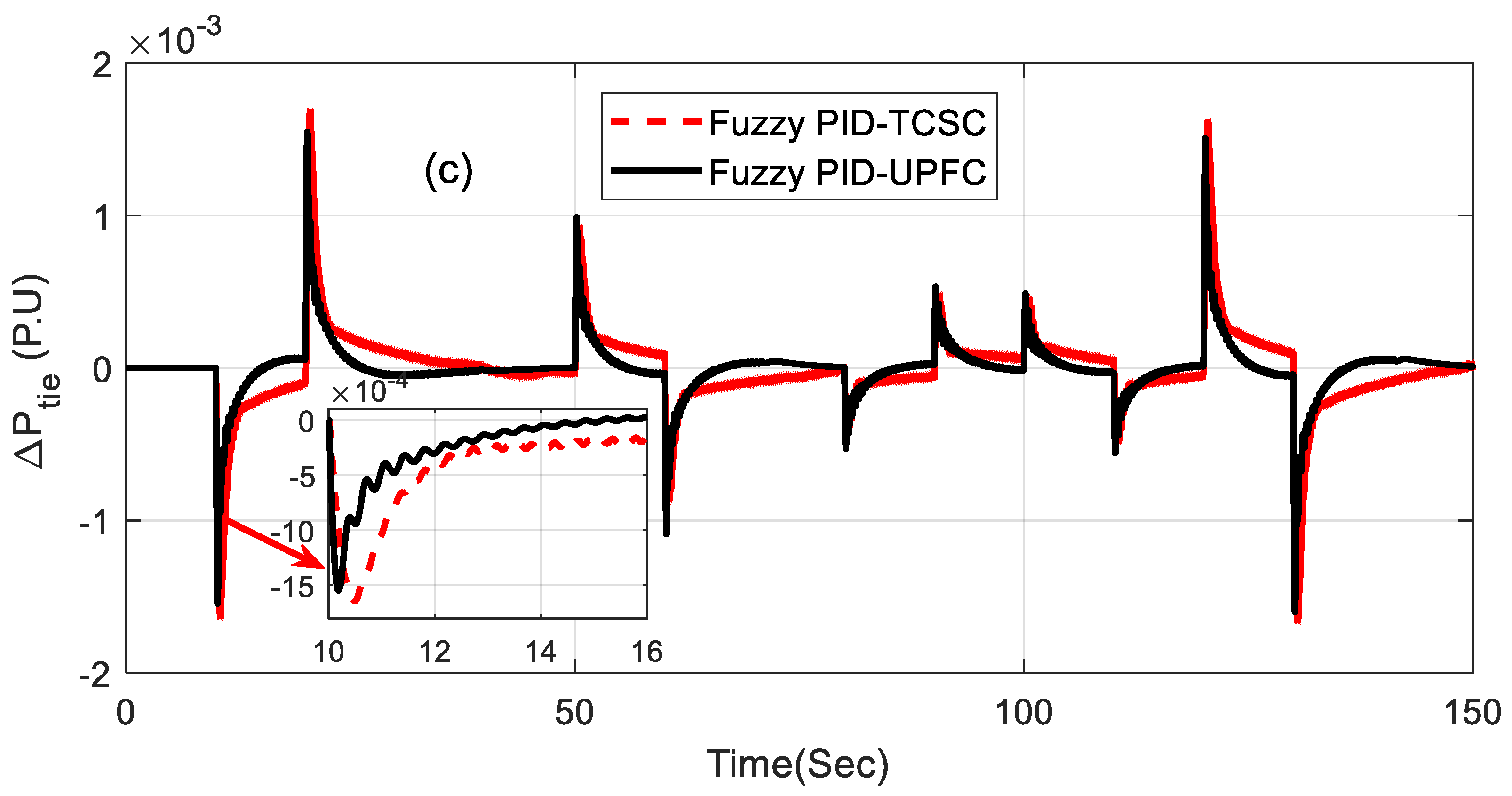
Originally, a dual-field hydro-thermal power scheme was studied and discussed in Section 2. A step load perturbation (SLP) of 1% was applied in area1 and fuzzy PID controllers were incorporated to minimize the frequency and tie-line power deviations. The optimal values of fuzzy PID controller parameters were obtained using the TLBO technique and the optimal values were finalized by employing various objective functions mentioned in Section 2. The performance index values obtained for the fuzzy PID controller were as follows: ISE= 0.0030; ITSE = 0.0060; IAE = 0.1901; ITAE = 0.8506. To improve the dynamic responses, different FACTS devices such as static synchronous series compensator (SSSC), thyristor-controlled series capacitor (TCSC), thyristor-controlled phase shifter (TCPS), and unified power flow controller (UPFC)were incorporated in the tie-line. The considered FACTS devices were connected in the tie-line to improve voltage stability and transient stability, as well as offer better power oscillation damping. For a better understanding, the single line diagram of the proposed power system with the UPFC device is shown in Figure 5. The parameters of the fuzzy PID controller for various cases are provided in Table 1, and the performance index values are tabulated in Table 2; Table 3. From Table 2 and Table 3, it is shown that the performance index values were reduced upon incorporating FACT devices. For the same system, smaller objective function values were obtained with the fuzzy PID with UPFC (ISE = 9.0459 × 10⁻⁵; ITSE = 1.0963 × 10⁻⁴; IAE = 0.0377; ITAE = 0.5600) when compared to the SSSC (ISE = 0.0011; ITSE = 0.0025; IAE = 0.1297; ITAE = 0.7814), TCPS (ISE = 0.0018; ITSE = 0.0037; IAE = 0.1500; ITAE = 0.7040), and TCSC (ISE = 0.0018; ITSE = 0.0024; IAE = 0.1266; ITAE = 0.6194). Table 3 also reveals that the values of settling time and under shoots were lower for the UPFC-incorporated system when compared to others.
The related dynamic performances of the system are shown in Figure 6a–c, where it can be noted that the system with the UPFC provided the best performance compared to others. The dynamic performance of the system was assessed for 1% SLP in area2 without retuning the control parameters, and the equivalent responses are shown in Figure 7a–c. The superiority of the system incorporated with a fuzzy PID and UPFC was also shown by evaluating the eigen values of the proposed system, as tabulated in Table 4. From the concept of relative stability, it is known that the system is better damped if it has more negative eigen values or if the poles of the congested loop scheme are further away from the imaginary axis. From Table 4, it can be noted that the eigen values of the UPFC structure were more adverse than the others and, therefore, it provided better damping.

Robustness Analysis

Robustness analysis was performed to realize the capacity of the controller for broad changes in the system’s parameters and operating conditions. This analysis was performed for the fuzzy PID controller with the UPFC-incorporated system as it performed better than the other systems. The system parameters and loading conditions were varied in the range of −25% to +25% without re-optimizing values of the fuzzy PID controller. The system performance index values such as the objective functions and settling times for 1% disturbance in area1 are provided in Table 5. From Table 5, it can be noted that the performance index values obtained under various conditions were more or less equal to the nominal values and, hence, the proposed controller can be considered a robust controller. The corresponding responses under various conditions are shown in Figure 8a–c and Figure 9a–c. From these figures, it can be pointed out that the responses of the system were sensitive to the variation in load and system parameters.
Furthermore, the effectiveness of the proposed controller was also analyzed by introducing a random step load as shown in Figure 10, and it was tested for the fuzzy PID controller with TCSC- and UPFC-incorporated systems, which showed superior performance. The step load disturbance was varied randomly from 0 s to 150 s, and the responses of the system were observed. In general, the frequency decreased when the load increased and viceversa. The best scenario considered the random load from 10 s to 20 s, as it increased when the system’s frequency decreased accordingly. The related responses in Figure 11a–c show how the system responded to a random step load. From these responses, it can be commented that the proposed controller can withstand any sudden changes in load disturbance.

5. Conclusions

An impact of FACTS devices was observed for the AGC problem of a two-area hydro-thermal power system. Non-linearities such as TD, GRC, and GRB for the two hydro and thermal units were included in the system for realistic analysis. A fuzzy PID controller was used as a secondary controller where the scaling factors and gain values were obtained using the TLBO technique. After testing the designed system with a fuzzy PID controller, FACTS devices such as SSSC, TCPS, TCSC, and UPFC were included in the tie-line to improve the results, and they were compared. The simulation results showed that the fuzzy PID plus UPFC-integrated system performed better than the others. The capability of the fuzzy PID plus UPFC was also investigated for variations in system parameters and random step load disturbances. Future work will focus on testing other metaheuristic optimization techniques for the proposed system. In addition, designing a type-2 fuzzy logic controller for the proposed system tuned with different bio-inspired metaheuristic techniques is another line of our future research.
In this paper, we tried to prove the fuzzy PID controller’s superiority over the traditional PID controller. As it is a new approach, its application was restricted to a two-area power system of equal area with two different units in each area interlinked by a tie-line. We tested its robustness and capability to handle non-linearities like transport delay (TD), generation rate control (GRC), and governor dead band (GDB) introduced in the system. The above approach can be extended to a multi-area power system with multiple sources in each area and it can also be tested with renewable energy sources in the system for the AGC problem. Although the fuzzy PID controller proved to be a better controller than traditional controllers with an increase in non-linearities in the system, it became a tedious process to simulate in the MATLAB/SIMULINK (9.1.0.441655, R2016b version, Mathematical computing software, Natick, Massachusetts, USA) environment. The time taken by the fuzzy PID system for each iteration is greater compared to the conventional PID system. Therefore, in the future, the aim will be to improve the time taken for each iteration. It is expected that fractional controller performance can be achieved by the proper tuning of controller parameters. In this regard, work can be planned on the application of evolutionary optimization techniques for the optimal configuration of fractional controllers.

Author Contributions

Ramana Pilla and Tulasichandra Sekhar Gorripotu proposed main idea of the paper and analyzed in MATLAB/SIMULINK environment. Ahmad Taher Azar has developed fuzzy system and extensively reviewed the manuscript. All authors read and approved the final manuscript.

Funding

This study was supported and funded by Prince Sultan University, Riyadh, KSA. We would like to show our gratitude to Prince Sultan University, Riyadh, KSA for funding the research project.

Conflicts of Interest

The authors declare no conflict of interest.

Appendix A

NomenclatureValue
iSubscript referred to area i (1, 2)
FNominal system frequency (Hz)60Hz
P R i Rated power of area i (MW)2000 MW
Δ F i Incremental change in frequency of area i (Hz)
Δ P D i Incremental step load change of area i
Δ P T i e Incremental change in tie-line power between areas 1 and 2 (p.u.)
A C E i Area control error of area i
B i Frequency bias parameter of area i (p.u. MW/Hz)0.425
T G i Speed governor time constant for thermal unit of area i (s)0.08
T T i Steam turbine time constant of area i (s)0.3
T P S i Power system time constant of area i (s)20
K P S i Power system gain of area i (Hz/p.u. MW)120
T 12 Synchronizing coefficient between areas 1 and 2 (p.u.)0.0113
K r i Steam turbine reheat constant of area i0.5
RRegulation parameter2.4
T r i Steam turbine reheat time constant of area i (s)10
T W i Nominal starting time of water in penstock of area i (s)1
T R S i Hydro turbine speed governor reset time of area i (s)5
T R H i Hydro turbine speed governor transient droop time constant of area i (s)0.513
T G H i Hydro turbine speed governor main servo time constant of area i (s)48.7
T F Teaching feature
t s i m Simulation time (s)50
a 12 P R 1 / P R 2 −1
a p f Area participation factor0.5

Appendix A.1. Transfer Function Model and Data for SSSC

Energies 12 04193 i001
K S S S C = 0.001; T S S S C = 0.03 s; T 1 = 0.2651 s; T 2 = 0.2011 s; T 3 = 0.6851 s; T 4 = 0.2258 s; T W = 10 s.

Appendix A.2. Transfer Function Model and Data for TCSC

Energies 12 04193 i002
K T C S C = 2; T T C S C = 0.02 s; J 12 = 0.05 ; k c = 0.5.

Appendix A.3. Transfer Function Model and Data for TCPS

Energies 12 04193 i003
K φ = 1.5; T T C P S = 0.1 s.

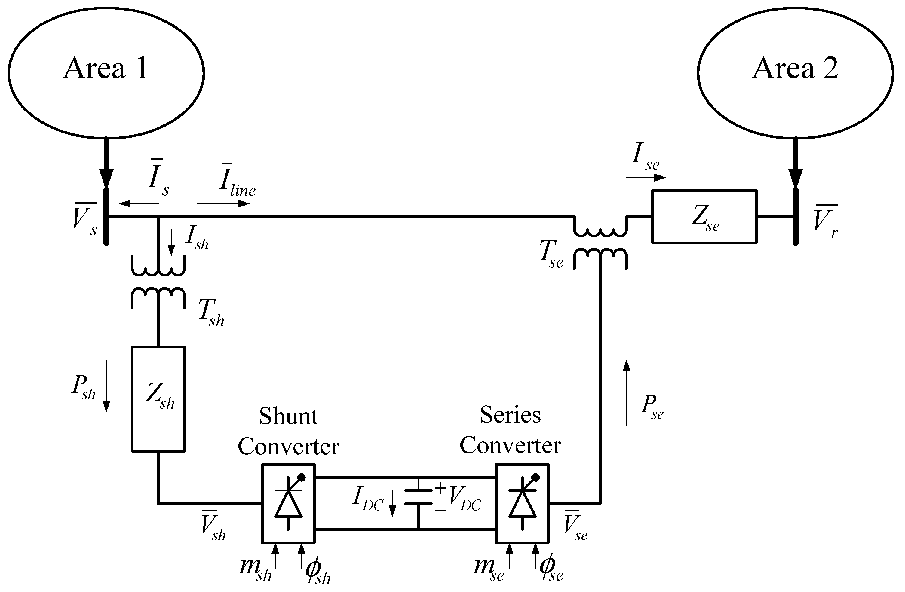
Appendix A.4. Transfer Function Model and Data for UPFC

Energies 12 04193 i004
T U P F C = 0.01 s.

References

  1. Elgerd, O.I. Electric Energy Systems Theory. An Introduction, 2nd ed.; Tata McGraw-Hill: New Delhi, India, 2007. [Google Scholar]
  2. Kasireddy, I.; Nasir, A.W.; Singh, A.K. IMC based controller design for automatic generation control of multi area power system via simplified decoupling. Int. J. Control Autom. Syst. 2018, 16, 994–1010. [Google Scholar] [CrossRef]
  3. Bevrani, H. Robust Power System Frequency Control; Springer: New York, NY, USA, 2009. [Google Scholar]
  4. Bevrani, H.; Hiyama, T. Intelligent Automatic Generation Control; CRC Press: Boca Raton, FL, USA, 2011. [Google Scholar]
  5. Shayeghi, H.; Shayanfar, H.A.; Jalili, A. Load frequency control strategies: A state-of-the art survey for the researcher. Int. J. Energy Convers. Manag. 2009, 50, 344–353. [Google Scholar] [CrossRef]
  6. Dev, A.; Sarkar, M.K. Robust higher order observer based non-linear super twisting load frequency control for multi area power systems via sliding mode. Int. J. Control Autom. Syst. 2019, 17, 1814–1825. [Google Scholar] [CrossRef]
  7. Rahmani, M.; Sadati, N. Two-level optimal load–frequency control for multi-area power systems. Int. J. Electr. Power Energy Syst. 2013, 53, 540–547. [Google Scholar] [CrossRef]
  8. Sonker, B.; Kumar, D. Dual loop IMC structure for load frequency control issue of multi-area multi-sources power systems. Int. J. Electr. Power Energy Syst. 2019, 112, 476–494. [Google Scholar] [CrossRef]
  9. Nosratabadi, S.M.; Bornapour, M.; Gharaei, M.A. Grasshopper optimization algorithm for optimal load frequency control considering Predictive Functional Modified PID controller in restructured multi-resource multi-area power system with Redox Flow Battery units. Control Eng. Prac. 2019, 89, 204–227. [Google Scholar] [CrossRef]
  10. Lu, K.; Zhou, W.; Zeng, G.; Zheng, Y. Constrained population extremal optimization-based robust load frequency control of multi-area interconnected power system. Int. J. Electr. Power Energy Syst. 2019, 105, 249–271. [Google Scholar] [CrossRef]
  11. Liu, J.; Yao, Q.; Hu, Y. Model predictive control for load frequency of hybrid power system with wind power and thermal power. Energy 2019, 172, 555–565. [Google Scholar] [CrossRef]
  12. Min-Rong, C.; Guo-Qiang, Z.; Xiao-Qing, X. Population extremal optimization-based extended distributed model predictive load frequency control of multi-area interconnected power systems. J. Frankl. Inst. 2018, 355, 8266–8295. [Google Scholar]
  13. Yin, L.; Yu, T.; Yang, B.; Zhang, X. Adaptive deep dynamic programming for integrated frequency control of multi-area multi-microgrid systems. Neurocomputing 2019, 344, 49–60. [Google Scholar] [CrossRef]
  14. Guha, D.; Roy, P.K.; Banerjee, S. Application of backtracking search algorithm in load frequency control of multi-area interconnected power system. Ain Shams Eng. J. 2018, 9, 257–276. [Google Scholar] [CrossRef] [Green Version]
  15. Fathy, A.; Kassem, A.M. Antlion optimizer-ANFIS load frequency control for multi-interconnected plants comprising photovoltaic and wind turbine. ISA Trans. 2019, 87, 282–296. [Google Scholar] [CrossRef] [PubMed]
  16. Pradhan, C.; Bhende, C.N. Online load frequency control in wind integrated power systems using modified Jaya optimization. Eng. Appl. Artif. Intell. 2019, 77, 212–228. [Google Scholar] [CrossRef]
  17. Khadanga, R.K.; Kumar, A. Analysis of PID controller for the load frequency control of static synchronous series compensator and capacitive energy storage source-based multi-area multi-source interconnected power system with HVDC link. Int. J. Bio Inspired Comput. 2019, 13, 131–139. [Google Scholar] [CrossRef]
  18. Guha, D.; Roy, P.K.; Banerjee, S. Study of differential search algorithm based automatic generation control of an interconnected thermal-thermal system with governor dead-band. Appl. Soft Comput. 2017, 52, 160–175. [Google Scholar] [CrossRef]
  19. Chandrakala, K.R.M.V.; Balamurugan, S. Simulated annealing based optimal frequency and terminal voltage control of multi-source multi area system. Int. J. Electr. Power Energy Syst. 2016, 78, 823–829. [Google Scholar] [CrossRef]
  20. Ali, E.S.; Abd-Elazim, S.M. BFOA based design of PID controller for two area load frequency control with nonlinearities. Int. J. Electr. Power Energy Syst. 2013, 51, 224–231. [Google Scholar] [CrossRef]
  21. Shabani, H.; Vahidi, B.; Ebrahimpour, M. A robust PID controller based on imperialist competitive algorithm for load-frequency control of power systems. ISA Trans. 2013, 52, 88–95. [Google Scholar] [CrossRef]
  22. Jin, Z.; Chen, J.; Sheng, Y.; Liu, X. Neural network based adaptive fuzzy PID-type sliding mode attitude control for a reentry vehicle. Int. J. Control Autom. Syst. 2017, 15, 404–415. [Google Scholar] [CrossRef]
  23. Gheisarnejad, M. An effective hybrid harmony search and cuckoo optimization algorithm based fuzzy PID controller for load frequency control. Appl. Soft Comput. 2018, 65, 121–138. [Google Scholar] [CrossRef]
  24. Sahoo, B.P.; Panda, S. Improved grey wolf optimization technique for fuzzy aided PID controller design for power system frequency control. Sustain. Energy Grids Netw. 2018, 16, 278–299. [Google Scholar] [CrossRef]
  25. Sahu, B.K.; Pati, T.K.; Nayak, J.R.; Panda, S.; Kar, S.K. A novel hybrid LUS–TLBO optimized fuzzy-PID controller for load frequency control of multi-source power system. Int. J. Electr. Power Energy Syst. 2016, 74, 58–69. [Google Scholar] [CrossRef]
  26. Khan, M.R.B.; Jagadeesh, P.; Jidin, R. Load frequency control for mini-hydropower system: A new approach based on self-tuning fuzzy proportional-derivative scheme. Sustain. Energy Tech. Assess. 2018, 30, 253–262. [Google Scholar]
  27. Rao, V.; Savsani, V.J.; Vakharia, D.P. Teaching-learning-based optimization: An optimization method for continuous non-linear large scale problems. Inf. Sci. 2012, 183, 1–15. [Google Scholar] [CrossRef]
  28. Esmaili, M.; Shayanfar, H.A.; Moslemi, R. Locating series FACTS devices for multi-objective congestion management improving voltage and transient stability. Eur. J. Oper. Res. 2014, 236, 763–773. [Google Scholar] [CrossRef]
  29. Singh, B.; Mukherjee, V.; Tiwari, P. A survey on impact assessment of DG and FACTS controllers in power systems. Renew. Sustain. Energy Rev. 2015, 42, 846–882. [Google Scholar] [CrossRef]
  30. Sang, Y.; Sahraei-Ardakani, M. Effective power flow control via distributed FACTS considering future uncertainties. Electr. Power Syst. Res. 2019, 168, 127–136. [Google Scholar] [CrossRef]
  31. Yu, S.; Chau, T.K.; Fernando, T.; Savkin, A.V.; Iu, H.H.-C. Novel quasi-decentralized SMC-based frequency and voltage stability enhancement strategies using valve position control and FACTS device. IEEE Access 2017, 5, 946–955. [Google Scholar] [CrossRef]
  32. Kavitha, K.; Neela, R. Optimal allocation of multi-type FACTS devices and its effect in enhancing system security using BBO, WIPSO & PSO. J. Electr. Syst. Inf. Technol. 2018, 5, 777–793. [Google Scholar]
  33. Dai, A.; Zhou, X.; Liu, X. Design and simulation of a genetically optimized fuzzy immune PID controller for a novel grain dryer. IEEE Access 2017, 5, 14981–14990. [Google Scholar] [CrossRef]
  34. Yesil, E.; Guzelkaya, M.; Eksin, I. Self-tuning fuzzy PID type load and frequency controller. Energy Convers. Manag. 2004, 45, 377–390. [Google Scholar] [CrossRef]
  35. Mudi, K.R.; Pal, R.N. A robust self-tuning scheme for PI-and PD-type fuzzy controllers. IEEE Trans. Fuzzy Syst. 1999, 7, 2–16. [Google Scholar] [CrossRef]
  36. Mudi, K.R.; Pal, R.N. A self-tuning fuzzy PI controller. Fuzzy Sets Syst. 2000, 115, 327–388. [Google Scholar] [CrossRef]
  37. Das, S.; Pan, I.; Das, S.; Gupta, A. A novel fractional order fuzzy PID controller and its optimal time domain tuning based on integral performance indices. Eng. Appl. Artif. Intell. 2012, 25, 430–442. [Google Scholar] [CrossRef] [Green Version]
Figure 1. Two-area thermal and hydro power model.
Energies 12 04193 g001
Figure 2. Structure of fuzzy PID controller.
Energies 12 04193 g002
Figure 3. Schematic of membership functions (MFs) for inputs and outputs.
Energies 12 04193 g003
Figure 4. Flowchart of teaching–learning-based optimization (TLBO) technique.
Energies 12 04193 g004
Figure 5. Single line diagram of two-area power system with unified power flow controller (UPFC).
Energies 12 04193 g005
Figure 6. (ac) Dynamic performance of 1% step load perturbation (SLP) in area1.
Energies 12 04193 g006aEnergies 12 04193 g006b
Figure 7. (ac) Dynamic performance of 1% SLP in area2.
Energies 12 04193 g007aEnergies 12 04193 g007b
Figure 8. (ac) Responses under loading variation.
Energies 12 04193 g008
Figure 9. (ac) Responses under Tg variation.
Energies 12 04193 g009
Figure 10. Random step load variation.
Energies 12 04193 g010
Figure 11. (ac) Responses under step load variation.
Energies 12 04193 g011aEnergies 12 04193 g011b
Table 1. Parameters of Fuzzy PID controller. SSSC—static synchronous series compensator; TCSC—thyristor-controlled series capacitor; TCPS—thyristor-controlled phase shifter (TCPS); UPFC—unified power flow controller.
Controller/ParametersFuzzy PIDFuzzy PID-SSSCFuzzy PID-TCPSFuzzy PID-TCSCFuzzy PID-UPFC
K10.30690.33461.31151.35140.4029
K20.74680.09950.83101.10990.1349
KP11.29901.91430.40370.84761.4560
KI10.84120.23960.23300.14261.2428
KD11.19291.58440.41030.23240.2516
K31.75360.53651.20960.71760.0003
K40.88230.10640.28250.02541.2729
KP20.69420.07561.87890.80730.4309
KI20.43531.96000.53870.04200.6168
KD20.07571.01550.30750.57390.0619
Table 2. Index values.
Type of ControllerTs (Sec)Us (−ve) (Hz)Us (−ve) (puMW)
∆F1∆F2∆PTie∆F1∆F2∆PTie
Fuzzy PID19.7118.3616.880.04080.0140.0036
Fuzzy PID-SSSC17.8718.1016.880.02710.0060.0002
Fuzzy PID-TCPS17.0722.354.760.02220.0150.0035
Fuzzy PID-TCSC15.6921.654.520.00770.0370.0765
Fuzzy PID-UPFC8.8417.354.280.00530.0070.0052
Table 3. Function values. ITAE—integral of time-weighted absolute error (ITAE); ISE—integral of squared error; ITSE—integral of time-weighted squared error; IAE—integral of absolute error.
Type of ControllersObjective Functions (JS)
J1 = ISEJ2 = IAEJ3 = ITSEJ4 = ITAE
Fuzzy PID0.00300.19010.00600.8506
Fuzzy PID-SSSC0.00110.12970.00250.7814
Fuzzy PID-TCPS0.00180.15000.00370.7040
Fuzzy PID-TCSC0.00180.12660.00240.6194
Fuzzy PID-UPFC9.0459 × 10−50.03771.0963 × 10−40.5600
Table 4. Eigen values of the proposed system.
Fuzzy PIDFuzzy PID-Fuzzy PID-Fuzzy PID-Fuzzy PID-
SSSCTCPSTCSCUPFC
−0.0250 + 0.9207i−33.3056−9.1524−47.4704−93.2746
−0.0250 − 0.9207i−5.015−0.4488 + 0.8518i−2.1673−10.7105
−0.0500 + 0.0000i−4.408−0.4488 − 0.8518i−0.4123−4.07
−2−0.0280 + 0.9190i−0.0500−0.05−0.0849
−1.9493−0.0280 − 0.9190i−2−2−2
−0.0205−0.1001−1.9493−1.9493−1.9493
−2−0.05−0.0205−0.0205−0.0205
−1.9493−2−2−2−2
−0.0205−1.9493−1.9493−1.9493−1.9493
−0.1−0.0205−0.0205−0.0205−0.0205
−3.3333−2−0.1−0.1−0.1
−12.5−1.9493−3.3333−3.3333−3.3333
−0.1−0.0205−12.5−12.5−12.5
−3.3333−0.1−0.1−0.1−0.1
−12.5−3.3333−3.3333−3.3333−3.3333
−12.5−12.5−12.5−12.5
−0.1
−3.3333
−12.5
Table 5. Performance index values under system parameter variation.
Variation of Parameter% ChangeSettling Time Ts (s)Obj
∆F1∆F2∆PTieITAE
Nominal08.8417.354.280.2433
Loading condition+258.8417.344.280.2433
−258.8317.344.280.2434
Tg+259.0517.504.250.2465
−258.4717.504.250.2391
Tt+258.2316.244.110.2327
−259.5218.948.010.3089
T12+259.3116.904.030.2394
−257.9017.964.340.2445

