Article

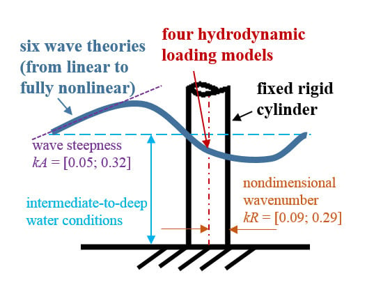
Comparison of Nonlinear Wave-Loading Models on Rigid Cylinders in Regular Waves

1
Department of Civil and Environmental Engineering, University of Florence, Via di S. Marta 3, 50139 Firenze, Italy
2
Energy and Environment Institute, University of Hull, Cottingham Rd, Hull HU6 7RX, UK
3
NTNU-AMOS & Center for Autonomous Marine Operation Systems, 7491 Trondheim, Norway
4
Institute of Marine Hydrodynamics, Harbin Engineering University, Harbin 150001, China
5
CNR-INM—Marine Technology Research Institute—National Research Council, Via di Vallerano 139, 00128 Rome, Italy
*
Author to whom correspondence should be addressed.
Energies 2019, 12(21), 4022; https://doi.org/10.3390/en12214022
Submission received: 3 October 2019 / Revised: 20 October 2019 / Accepted: 21 October 2019 / Published: 23 October 2019

Abstract

:
Monopiles able to support very large offshore wind turbines are slender structures susceptible to nonlinear resonant phenomena. With the aim to better understand and model the wave-loading on these structures in very steep waves where ringing occurs and the numerical wave-loading models tend to lose validity, this study investigates the distinct influences of nonlinearities in the wave kinematics and in the hydrodynamic loading models. Six wave kinematics from linear to fully nonlinear are modelled in combination with four hydrodynamic loading models from three theories, assessing the effects of both types of nonlinearities and the wave conditions where each type has stronger influence. The main findings include that the nonlinearities in the wave kinematics have stronger influence in the intermediate water depth, while the choice of the hydrodynamic loading model has larger influence in deep water. Moreover, finite-depth FNV theory captures the loading in the widest range of wave and cylinder conditions. The areas of worst prediction by the numerical models were found to be the largest steepness and wave numbers for second harmonic, as well as the vicinity of the wave-breaking limit, especially for the third harmonic. The main cause is the non-monotonic growth of the experimental loading with increasing steepness due to flow separation, which leads to increasing numerical overpredictions since the numerical wave-loading models increase monotonically.

Graphical Abstract

1. Introduction

Wind has become a strong player in the energy field but its main limiting factor for growth, especially for offshore technologies, remains the cost. Since the support structures are the most expensive part of offshore wind turbines (OWTs), advancements in the modelling of wave-loading could lead to safer and more cost-efficient future designs. Most commonly installed monopile-supported OWTs are normally placed in shallow to intermediate waters, where wave nonlinearities gather and may lead to dangerous nonlinear resonant amplifications of the dynamic response, such as ringing.
Ringing is a non-Gaussian resonant response occurring after the passage of a particularly steep wave, reaching its maximum within a burst of a few oscillations and dissipating slowly [1,2]. Such resonant amplifications cause significant strain on the offshore structure, causing increased fatigue and reduced remaining useful lifetime. Ringing is normally associated with third-order wave-loading [1,2,3] although it has been suggested to be caused by higher-order loading components as well [4,5]. The higher-order force components associated with ringing have been observed to be much larger in shallower water than deep [6,7], reiterating the importance of its consideration in the shallow to intermediate water depths where monopile-supported OWTs are placed. The applicability of this dangerous resonant phenomenon to the OWT substructures is highlighted by the fact that the structural frequency of the monopile-supported offshore wind turbines falls in the range of 3rd harmonics of typical rough sea states occurring at sites where OWTs are placed.
Ringing is a dynamic amplification of the structural response, therefore cannot be observed on a fixed, rigid cylinder. Nonetheless, in several past studies a fixed cylinder has been investigated in the same wave conditions where ringing is expected, and observed a phenomenon of strong forcing nonlinearities named “secondary load cycle” ( s l c ) [2,3,4,5,6,8,9]. s l c appears as a secondary peak in the loading, around one quarter after the main peak and has been initially associated with ringing. There has been a dispute over what the secondary load cycle is governed by: some suggesting Froude number [3,4], some wave steepness [2], some viscous effects [10,11], while others called it a ‘hydraulic jump’ due to local wave breaking [5,8]. Most of the early research neglected diffraction [2,3,4,5,8] but in a recent computational study Paulsen et al. (2014) [6] have shown that the secondary load cycle is actually caused by the interaction between the opposing flows—the outer still continuing in the direction of the propagating wave, and the inner inside a vortex which formed at the back of the cylinder due to diffracted wave—creating a reduction in pressure which is observed as the secondary load cycle. The three-dimensional CFD study was the only method to capture s l c numerically to date. A suggestion was made to disassociate ringing from secondary load cycle on the grounds that even the first six harmonics of the loading did not recreate the secondary load cycle while ringing is commonly associated with the third [6]. This suggestion was later confirmed experimentally by Suja-Thauvin et al. (2017) [9], where ringing was repeatedly observed without the occurrence of secondary load cycle in the same wave events on two parallel cylinders—fixed and moving. Therefore the ability to numerically recreate s l c does not indicate on the ability of the models to capture ringing; nonetheless, since this paper focuses on the suitability of wave-loading models for a fixed cylinder in steep waves, their capability to capture s l c is investigated as well.
Ringing on offshore wind turbines has been numerically captured with fully nonlinear wave kinematics, but repeatedly shown to be omitted if linear wave kinematics were used [7,12,13,14,15]. Moreover, Marino et al. (2014) [14] have recently shown that second-order wave kinematics are not sufficient to capture ringing either. Nonetheless, the nonlinearities in wave-loading stem not only from the wave kinematics but also from the hydrodynamic loading model, and it should be noted that these previously noted studies have all used Morison equation [16] as the hydrodynamic loading model [7,12,13,14,15]. However, in the 1990s more advanced hydrodynamic loading models than Morison equation were proposed. One of such is Rainey theory [17,18], which suggests neglecting the drag term from the Morison equation and correcting the linear Morison inertia term to third order by nonlinear slender-body terms, which consider nonlinear flow and free-surface effects to second and third order. Higher-order hydrodynamic loading models were also derived as perturbation theories, best known of which are Malenica & Molin (M&M) [19] and Faltinsen–Newman–Vinje (FNV) [20]. They are both derived directly to third order to take the ringing-associated nonlinearities and wave diffraction into account. The main difference between them is that FNV assumes the radius of the structure to be of the same order as the wave amplitude (both of the order O ( ϵ ) with ϵ < < 1 ) while the wavelength λ is of order O ( 1 ) [19,20]. An important contribution in the FNV comes from the nonlinear scattering potential deriving from the free-surface conditions. However, by disregarding this effect, the main difference between the formulation in [17] and the one in [20] relies in the different way the loads are derived, i.e., through direct integration of the pressure and Gauss integral theorem in [20] and momentum and energy conservation in [17].
The influence of nonlinearities in hydrodynamic loading models and in wave kinematics have often been treated as separate issues. For example, in Chaplin et al. (1997) [2] the suitability of Morison equation and Rainey model were tested against the results of accurate experiments, both hydrodynamic loading models with a 16th order stream-function theory for the wave kinematics. In Stansberg (1997) [21], on the other hand, FNV theory was the only numerical loading model. A wide selection of wave kinematics and hydrodynamic loading models were compared in the OC5 Phase Ib [7], but none of them was a consistent perturbation model, e.g., FNV or M&M. Swan et al. (2002) [22] compared Morison equation and Rainey corrections on linear and fully nonlinear wave kinematics and determined that the nonlinearities in wave kinematics were more important than the nonlinearities in the hydrodynamic loading model because when the wave kinematics were fully nonlinear, the nonlinear corrections in the loading model became less relevant. The closest set-up to the present study has been conducted by the Wave Loads project [23] where Morison equation, Rainey theory, FNV and M&M were compared using fully nonlinear wave kinematics. However, the aim of the study differed, hence also the range of the kinematics considered in it. Moreover, at the time of the project [23] only the deep-water FNV formulation [20] was available, therefore it only provided meaningful comparison in high water depths instead of shallow to intermediate. Only recently, indeed, Kristiansen and Faltinsen [24] introduced the FNV formulation for finite water depth. It is observed that in [24] the waves were up to intermediate steepness, therefore secondary load cycle was not observed, leaving the finite-depth FNV loading model not assessed in a study on ringing or secondary load cycle to this date.
Therefore, the present work provides a detailed study of the distinct influences on the wave-loading stemming from the nonlinearities in wave kinematics and in the hydrodynamic loading models considering different wave and water depth conditions. The objective is to understand which nonlinearities are more influential in the ringing phenomenon, but also to improve the numerical modelling of the wave-loading on OWT monopiles in general. A systematic study is presented considering a range of increasingly nonlinear wave kinematics as input to a selection of hydrodynamic loading models with nonlinear corrections. Six models for wave kinematics (Section 2.1) and three hydrodynamic loading models (Section 2.2) are used in this study, on a grid of experimental values, presented in Section 2.3. Main topics analyzed in this study of regular wave-loading on a rigid cylinder are presented in Section 3. Section 3.1 focuses on the capability to capture secondary load cycle numerically, while Section 3.2 clarifies the distinction between the nonlinearities stemming from the wave kinematics and from the hydrodynamic loading model. Section 3.3 and Section 3.4 discuss the suitability of the wave-loading models to recreate experiments, especially in the off-design values for the theories over increasing steepness and nondimensional wavenumber consequently. Section 3.5 then summarizes the findings over the experimental grid, determining the best-suited wave-loading models and distinguishing the areas where which influence is dominant. Finally, Section 4 lists the conclusions along with remarks on limitations and future work.

2. Methodology

In this study, six wave kinematics and four hydrodynamic loading models from three theories are compared with experimental data found in the literature. The wave-loading model is therefore defined as the combination of selected wave kinematics and a selected hydrodynamic loading model. Each is introduced in short in this section.

2.1. Wave Kinematics

The modelling of linear and weakly nonlinear wave kinematics is made using Airy, Stokes 2nd, Stokes 3rd and Stokes 5th order wave theories [25]. The stretching of kinematics from still water level to the instantaneous free surface follows the Taylor expansion as described in [24]. The fully nonlinear wave kinematics are based on the perturbation theory by Rienecker–Fenton (R–F) [26], as well as computed in a two-dimensional higher-order Boundary Element Method (BEM) model initialized with the same R-F theory. The BEM model [27,28,29] is based on a two-step mixed Eulerian-Lagrangian solution scheme and employs quadratic boundary elements in the Eulerian step to solve the Laplace equation, and the fourth order Runge–Kutta for the time integration in the Lagrangian step. Potential continuity at corner points [30] and 5-point smoothing [31] in simulations with higher wave steepness are used to prevent numerical instabilities such as “sawtooth”.
Throughout the study the different wave kinematics are denoted by color of the marker or line: linear—black, Stokes second order—blue, Stokes third order—green, Stokes fifth order—cyan, Rienecker–Fenton—red, BEM—dark red.

2.2. Hydrodynamic Loading Models

The comparison of hydrodynamic loading models is conducted between three commonly implemented theories: Morison equation, Rainey theory, and FNV perturbation theory. Each model is denoted throughout the study by the style of the line or marker.
Morison equation [16] consists of linear inertia term M and quadratic drag d. Since the experimental conditions recreated in this paper fall in the inertia and diffraction regimes (see Section 2.3), drag contribution is neglected. Therefore, Morison equation consists of linear inertia term only, which is integrated up to the instantaneous wave elevation, as illustrated in Figure 1a and described in Equation (1).
F M o r i s o n = F M = h η C m ρ π R 2 u t d z ,
where η is the instantaneous wave elevation, h—water depth, ρ —water density, R—cylinder radius and u—horizontal velocity of the water particles.
The inertia coefficient C m is considered depth-independent because of the constant circular cylinder section considered along the water depth. Its value is chosen as C m = 2 in all cases for the consistency across experiments and hydrodynamic loading models. In the following, results obtained with Morison equation are marked with a solid line or circle markers.
Slender-body theory [17,18] corrects the Morison inertia term M (Equation (1)) to third order. Following the formulation of [2], the corrections are: axial divergence force A (Equation (2)), integrated from the sea bottom to the instantaneous wave elevation; surface intersection force I (Equation (3)), and surface distortion force D (Equation (4)), both applied as point loads at the instantaneous wave elevation, as illustrated in Figure 1a.
F A = h η ρ π R 2 w z u d z
F I = ρ π R 2 2 u 2 η x
F D = 7 ρ π R 2 2 g u 2 u t
The derivation of the A and I terms is based on the expansion of k R term instead of the usual k A , giving the advantage of no limitation in terms of steepness [18]. However, the derivation of the surface distortion term D, which is the third-order term in this theory, rests on Stokes small amplitude assumption [2,18]. Therefore, numerous authors have doubted its suitability in very steep waves and have refrained from adding it, applying only the A and I terms instead, e.g., [2,15]. Thus, in this study both M + A + I (MAI) and M + A + I + D (MAID) combinations are modelled to assess the suitability of both variations of the Rainey theory. Throughout this study MAI is denoted by dotted line or diamond markers, while MAID by dash-dot line or cross markers.
FNV theory was originally derived for regular waves in 1995 [20] but quickly expanded to irregular in 1996 [32], after which further generalizations followed for general cross-sections in 1999 [33] and recently for finite depth in 2017 [24]. In this study, the finite-depth formulation of the FNV theory is implemented, which is valid for regular and irregular waves as well as numerical wave tanks [24]. As illustrated in Figure 1b, the total horizontal force F F N V , listed in Equation (5), consists of two main components: force F (Equation (6)), integrated from the sea bottom to the instantaneous free-surface elevation, and a point load F ψ (Equation (7)) due to the nonlinear potential ψ , which is applied at the still water level in consistency with the original theory [20]. It is worth noting that the integrated force F includes components of nonlinear loading due to wave kinematics (first term in (Equation (6)) as well as the effect of infinite-frequency hydrodynamic added mass (second term in (Equation (6)).
F F N V = h η F ( z , t ) d z + F ψ ,
where
F = ρ π R 2 ( u t + u u x + w u z ) + a 11 ( u t + w u z ) ,
where a 11 is the two-dimensional added mass coefficient, and
F ψ = 4 ρ π R 2 g u 2 u t .
It can be seen that if the nonlinear terms in the distributed force F were excluded, the F force with only the two u t terms would be equal to the Morison inertia term F M with the inertia coefficient C m = 2 . Therefore, the difference between the FNV theory and Morison equation is the assessment of these nonlinear integrated terms and the point load F ψ . The difference between the finite-depth FNV and the Rainey theories, as discussed by Kristiansen and Faltinsen (2017) [24], is the point load F ψ . The surface distortion term D in the Rainey theory (Equation (4)) has a very similar formulation to this point load F ψ (Equation (7)) with the coefficient of 3.5 instead of 4, but with a crucial difference of the point of application—at the instantaneous free surface for D and at the still water level for F ψ .
The theory is derived directly to third order with which ringing is associated, and considers diffraction, by which secondary load cycle has been explained in [6], therefore could be expected to have a strong potential to recreate the secondary load cycle numerically. The marking for FNV theory in this study is a dotted line or star marker.

2.3. Experimental Grid

Multiple experiments from literature on a fixed rigid surface-piercing cylinder are investigated in this study as shown in Figure 2 on the ( k A , k R ) -grid, where k denotes the linear wave number, A—linear wave amplitude, R—cylinder radius. First of all, two cases of extremely high steepness from Grue and Huseby (2002) [4] are considered because they fall right in the center of the previously reported conditions where secondary load cycle and ringing occur [4], as well as provide an insight into the conditions with extremely high steepness of k A > 0.3 . In addition, the experimental campaign by Kristiansen and Faltinsen (2017) [24] systematically covers the steepness up to ≈0.165 and a range of k R values, while the experiments by Stansberg (1997) [21] allow assessment of the intermediate-to-high steepness between the previously mentioned experimental campaigns, as well as the influence of the cylinder radius—therefore the k R number—in the same wave conditions. For the sake of brevity, the experimental details are not reported here but can be found in the original papers. The numerical values for wave period T and wave amplitude A were selected as reported in the original papers, with the only exception of the two cases of Grue and Huseby (2002) [4], where the numerical wave height H and period T were tuned by matching the digitized wave elevation, superimposed at zero-upcrossings, by the lowest root-mean-square-error.
The grid is divided into the diffraction, inertia and drag regimes by the linear Keulegan–Carpenter K C number values equal to π and 10, where K C number is defined as u H 1 / D c y l , where u is the linear horizontal wave velocity, H 1 is the linear wave height, and D c y l is the diameter of a cylinder. The experiments are scattered over the diffraction and inertia regimes, which is appropriate since Morison and Rainey loading models are inertia-based, and FNV is diffraction-based. It is of interest to note that most of the previously reported cases of observed secondary load cycle fall in the inertia regime, justifying numerous authors discussed in the introduction neglecting wave diffraction. As discussed in [2], Stokes first-order diffraction effects are only expected to start at k R 0.5 , therefore strongly outside of the considered range, while the Stokes third-order diffraction effects could in theory be applicable from as low k R as 0.05 (defined by Malenica and Molin (1995) [19]), but the derivation of this threshold rests on perturbation scheme therefore it would be expected to lose validity at such high steepness where local wave breaking is expected. Nonetheless, the s l c has been surprisingly explained by a diffracted wave by Paulsen et al. (2014) [6], justifying the investigation of diffraction-based loading models in the theoretically inertia regime.
The currently analyzed experiments are also compared to the limits of wave theories, as defined by IEC 61400-3 Design requirements for offshore wind turbines [34] in Figure 3, where H is the wave height, g—gravitational constant, T—wave period, h—water depth. All the experiments fall in the intermediate to deep-water conditions, therefore the shallow water limitations are avoided. They also fall outside of the range of the linear and second-order kinematics, therefore the nonlinearities in wave kinematics are expected to matter. Lastly, it is evident that the cases in intermediate water depth are closer to the wave-breaking limit despite the smaller wave height, and thus the recommended wave theories are even higher.

3. Results and Discussion

This section is the core of the study where the following three main issues are addressed: (1) the capability to numerically capture secondary load cycle, in Section 3.1; (2) the distinction between the nonlinearities stemming from the wave kinematics and from the hydrodynamic loading model, in Section 3.2; (3) the suitability of the wave-loading models to recreate experiments, especially in their off-design conditions: as steepness increases in Section 3.3, and as the k R number increases in Section 3.4; and the overall behavior of the numerical loading models on the grids of wave theory limits and the wave and cylinder conditions in Section 3.5.

3.1. Secondary Load Cycle

In Figure 4 the grey dotted lines show the experimental values of the superimposed wave elevation (Figure 4a) and horizontal forcing (Figure 4b) for the case with wave steepness k H / 2 = 0.31 and wave period T = 0.85 s . This case corresponds to the Grue and Huseby (2002) [4] case, which was seen to fall among the previously observed s l c range, shown in Figure 2. The s l c can be seen to occur around t = [ 0.5 0.75 ] s in the experimental loading (Figure 4b).
A past preliminary study [35] has already shown that not even with fully nonlinear BEM wave kinematics with Morison equation (inertia only as well as full formulation including quadratic drag) or Rainey theory manage to capture the secondary load cycle. In this extended study the newly derived finite-depth FNV theory was also considered, and is therefore shown in Figure 4b with linear and fully nonlinear wave kinematics as input (dashed black and dark red lines). It is compared with Morison inertia term, also with linear and fully nonlinear wave kinematics as input (solid black and dark red lines).
The fact that FNV theory omits the secondary load cycle just like the other loading models, even with fully nonlinear BEM wave kinematics, indicates that secondary load cycle is caused by either three-dimensional effects or loading higher than third order. Nonetheless, as recently suggested from the numerical study by Paulsen et al. (2014) [6] and later confirmed experimentally by Suja-Thauvin et al. (2017) [9], the secondary load cycle, even though it occurs in the same wave conditions, is not directly linked to ringing. Therefore, the fact that s l c is not captured by any of the analyzed combinations of wave models does not imply that ringing is omitted too.

3.2. Distinction between the Nonlinearities in Wave Kinematics and Loading Models

A deeper understanding of where the predominant nonlinearities in loading are stemming from—wave kinematics or the loading model—is crucial in the study of ringing and optimization of numerical wave-loading models.
The importance of nonlinearities in wave kinematics to capture the nonlinear wave profile of this extremely steep wave is evident from Figure 4a. The fully nonlinear wave kinematics closely capture the experimental wave-loading, while linear wave kinematics are limited to sinusoidal profile which does not recreate the steeper crest and shallower trough. The strong influence of nonlinearities on the total wave-loading is seen in Figure 4b: the nonlinearities in the wave kinematics reduce the total loading (comparing dark red lines with the corresponding black lines), while the nonlinearities in the hydrodynamic loading model cause an increase of the loading, especially at the peak of the loading where higher harmonics normally appear (comparing the dashed lines with corresponding solid lines).
Nonetheless, a deeper insight is easier from the harmonic analysis, which is given in Figure 5 for wave elevation (top row) and horizontal loading (bottom row), for the first five harmonics (left to right). The harmonic analysis for the wave elevation (Figure 5a–e) shows, as expected, that linear wave kinematics (black markers) are negligible in the higher harmonics (Figure 5b–e), and therefore overestimate the first harmonic (Figure 5a). It is worth noting here that, as introduced in Section 2.3, in this extremely steep and unstable case the wave characteristics for numerical models were tuned to match the superimposed wave elevation with lowest root-mean-square-error. The fully nonlinear wave kinematics (dark red markers), on the other hand, capture the experimental wave elevation values much closer, even in the high harmonics.
The harmonic analysis of wave-loading (Figure 5f–j) reveals the influence of hydrodynamic loading models as well. Even the most linear hydrodynamic loading model, Morison inertia term (Equation (1)) in combination with linear wave kinematics (black circle) leads to a second-order peak (Figure 5g) due to the integrated wave acceleration profile over depth (see Equation (1)). The higher harmonics (Figure 5h–j), nonetheless, are negligible. This most linear case (black circle) is taken as reference case for assessing the influence of nonlinearities in wave kinematics and hydrodynamic loading models.
The effect of wave nonlinearities is seen from the wave forcing with the same Morison equation, but with BEM kinematics (dark red circle, compared to black circle). It can be seen that the nonlinearities in wave kinematics reduce the first harmonic (Figure 5f), but increase all the higher harmonics (Figure 5g–j), similarly as seen with the impact on wave elevation (Figure 5a–e). Meanwhile, the nonlinearities in the hydrodynamic loading model can be seen from the loading with linear wave kinematics, but more nonlinear FNV theory (Equation (5), black star markers compared to black circles). It can be seen that the nonlinearities in hydrodynamic loading model increase the loading in all harmonics (Figure 5f–j). It should be noted that FNV is a third-order perturbation theory, therefore the harmonics above third (Figure 5i–j) are not affected, while with Rainey theory [17,18] the fourth and fifth harmonics increased. Finally, the effect of combined nonlinearities is seen from BEM kinematics with FNV loading model (dark red star markers, compared with black circles), and it is to increase all higher harmonics (Figure 5g–j). It can be seen that it leads to the highest total loading from the second harmonic (Figure 5g), increasing with the increasing harmonics (Figure 5h–j). Swan et al. (2002) [22] found that when fully nonlinear wave kinematics were used (Rienecker–Fenton in [22]), the nonlinearities in the hydrodynamic loading model (Rainey theory in [22]) were of smaller importance. In this study, nonetheless, as will also be seen in next sections, the importance of the nonlinearities in the hydrodynamic loading model is found to be greater for the more nonlinear wave kinematics than for linear.
To show the influence of the distinct nonlinearities over the increasing steepness Figure 6 shows a representative case in intermediate water depth, which corresponds to the wave settings of Kristiansen and Faltinsen (2017) [24] (wave period T = 2.021 s , water depth h = 0.546 m , increasing wave steepness). In Figure 6 the experimental values are excluded, since the behavior of the numerical models with regards to the other numerical models, ignoring the experimental values, is similar across different settings of wave periods and water depths. The loading in each harmonic is additionally normalized by wave steepness H 1 / λ (where H 1 is the linear wave height and λ is the linear wavelength) to the power of that harmonic.
In theory the numerical wave-loading increases monotonically with the increasing wave steepness, which would appear as a horizontal line on graph with such normalization. Therefore, the deviating curvatures are representing the effect of the nonlinearities in the wave kinematics and hydrodynamic loading models. It should be noted that the first harmonic is actually predicted rather similarly by all numerical models and the modelled loading is actually increasing rather monotonically with the increasing steepness. These curvatures are emphasized by the very small range of values in the vertical axis allowing easier illustration of the underlying principles.
As seen from Figure 6a, in the first harmonic the most horizontal line and the reference case is the Morison equation, i.e., linear inertia term, with the linear wave kinematics (black circle). It can be seen from the nonlinear kinematics (all colors except black (linear) and blue (second order)) that the effect of the nonlinearities in the wave kinematics to reduce the first harmonic (Figure 6a) is becoming larger with increasing steepness. On the contrary, as seen from Figure 6b,c, the effect of increasing the loading in higher harmonics is decreasing as the steepness increases. The fact that second-order wave kinematics (all blue markers) are the only exception, which increases the loading at any given steepness and becomes larger as the steepness goes up, could potentially be explained by the fact that the second-order Stokes-wave kinematics do not get the nonlinear correction to the wave number and wave celerity as the higher-order nonlinear wave kinematics get.
The influence of the nonlinearities in the hydrodynamic loading model—to increase the loading in all harmonics—is seen to persist and increase as steepness increases (compare, for example, MAID model (crosses) with the Morison equation (circles) in any wave kinematics (any color)) in all panels of Figure 6. The only exception is the FNV loading model (star markers), which in certain conditions has the capability to correct the Morison equation (circles) towards the reduction of the loading, e.g., see the star markers in Figure 6b, especially at the lowest steepness. It can also be observed that the nonlinearities in the hydrodynamic loading models, growing most with the increasing wave steepness, are the both third-order hydroloading models MAID (crosses) and FNV (stars), observed most clearly with the second-order wave kinematics (blue color) in the second and third harmonics (Figure 6b,c).

3.3. Non-Monotonic Experimental Behavior Over Increasing Steepness

As just established in Section 3.2, the numerical results increase relatively monotonically with increasing steepness. Nonetheless, as seen from Figure 7 which includes the experimental results, the behavior of the experimental results does not follow the same trend.
Figure 7 shows the FFT analysis of the first three harmonics (from top to bottom) of the normalized horizontal force ( F x / ( ρ g R 3 ) ) over increasing steepness H 1 / λ for three periods of T = 1.443 s (left), T = 1.732 s (middle) and T = 2.021 s (right) for the depth of h = 0.397 m . It is worth mentioning that experimental values for depth h = 0.564 m were also provided in [24], but they are omitted from this paper for brevity due to similar behavior. The case of h = 0.397 m is kept because the cases in shallower water become more nonlinear at lower steepness, allowing a more detailed analysis. It should also be noted that in Figure 7 the normalization does not divide by the steepness to the power of the harmonic, as in the Figure 6 before, and the y-axes are fixed for each harmonic for the ease of comparison.
It should be noted that in the experimental wave setting with longest wave period T = 2.021 s (Figure 7c,f,i) wave breaking was reported in the steepest four cases (final four grey dots on the right of Figure 7c,f,i). The occurrence of wave breaking nearly coincides with the theoretical upper limit of the Stokes fifth-order theory, defined as Ursell number U r = 40 ( U r = H 1 λ 2 / h 3 ), indicated by a vertical dotted line. Except for the breaking wave cases, the first harmonic (Figure 7a–c) is captured well enough by all kinematics and loading models. In more detail the experimental values at the higher steepnesses are better captured by the nonlinear wave kinematics regardless of the hydrodynamic loading model, while the linear and second-order kinematics tend towards overestimation.
The second harmonic (Figure 7d–f) already shows an extremely non-monotonic behavior. The cases of breaking waves aside, after a certain steepness the total loading is hardly increasing with the increasing steepness. Some of the cases are showing such small increment in the total loading over the increasing steepness that the monotonically increasing linear wave kinematics with nonlinear loading models, e.g., MAID (black cross) or MAI (black diamond), are becoming the closest-predicting models. In the third harmonic (Figure 7g–i) such effect is amplified even more, especially in the cases with the largest k R number, where even the linear kinematics with the MAID model (black cross) are overestimating the loading (see Figure 7i). In Kristiansen and Faltinsen (2017) [24] the discrepancies are explained by flow separation, although the addition of drag and reduction of mass coefficient corresponding to the local K C numbers did not offer a correcting solution to the FNV theory regardless of whether third or fifth-order wave theory was used [24]. The main contribution of this paper on this discussion is that a wider range of wave theories and loading models are also increasing monotonically with wave steepness and therefore overpredicting the higher harmonics at the occurrence of the non-monotonic growth of the experimental results with increasing steepness.
To better understand the limiting steepness at which the agreement between the loading models and the experimental values ceases, vertical lines representing K C = π were added. The sub- and superscripts represent which maximum horizontal velocity was used for its calculation: linear ( K C 1 ), fifth order taken at the crest ( K C 5 + ), or fifth order taken at the trough ( K C 5 ). In fact, the change in behavior falls within that range, although the exact K C number depends on the specific case. The general trend is that the change in the experimental behavior starts earlier for lower k R numbers. This again is represented well in the wave limits graph in Figure 3—lower k R numbers bring the cases towards shallower waters and closer to the wave-breaking limit, where even the lower wave steepness makes the numerical loading models become inappropriate. The worrying finding is, however, that since even more nonlinear wave theories are suggested in such wave conditions by the International Standards [34], the overprediction would be increased even more.
As discussed in [24], such discrepancy between the numerical and experimental loading was also observed in deep water in third harmonic by Huseby and Grue (2000) [36]. The deep-water cases in this study by Stansberg (1997) [21] are shown in Figure 8. It shows the comparison with the experimental results from [21] for the period T = 2.10 s over the increasing steepness for both radii ( R = 0.1 m and R = 0.1635 m ), normalized by the cylinder radius R squared times the linear amplitude A to the power of the harmonics. The first three harmonics are shown from left to right, and the y-axes are fixed to the same value across the harmonics.
The first harmonic is captured well in all steepnesses for both cylinders, therefore a zoom is provided in the same panel (Figure 8a). Only the highest steepness starts to get overestimated by the MAID model (crosses) and underestimated by Morison equation (circles). The experimental values in the second harmonic (Figure 8b) display a distinct non-monotonic behavior, and also strongly differ for the different cylinder radius even at the lowest steepness with more nonlinear loading models fitting better the smaller radius (light grey dot), and the Morison equation (circles) fitting best for the larger radius (dark grey dot). As the steepness increases the second harmonic starts to get strongly overestimated by all models, a behavior already seen in the comparison with Grue and Huseby (2002) [4] in Figure 5g with even higher steepness, hence even closer to the wave-breaking limit. It is worth noting that in contrast to Kristiansen and Faltinsen (2017) [24] linear wave kinematics are still suitable in capturing the second harmonic, potentially due to the larger distance from the wave-breaking limit despite the larger steepness and due to deeper depth (refer to Figure 3). Third harmonic (Figure 8c) is surprisingly well captured, in contrast to the intermediate depth cases (Figure 7). Yet again the non-monotonic behavior is seen and as the steepness increases less nonlinear loading models are capturing the loading better. On the contrary to the second harmonic, in the third harmonic the larger cylinder shows higher loading than the smaller cylinder, therefore more nonlinear loading models suiting it better, decreasing in nonlinearity as the steepness increases.
A notable difference of these deep-water cases from the cases in intermediate water depth by Kristiansen and Faltinsen (2017) [24] (Figure 6 and Figure 7) is that the hydrodynamic loading models have a much stronger influence than wave kinematics, especially in the first harmonic. For example, in deep water (Figure 8a) regardless of which wave kinematics were used, the final loading is similar for all wave kinematics with the same hydrodynamic loading model, while in intermediate water depth (Figure 6a) the models are grouped by the kinematics. This could be explained by looking at the graph of wave theory limits in Figure 3, where the cases shown in Figure 6 refer to the dark blue crosses while the cases shown in Figure 8 refer to the green circles. It can be seen that the Stansberg (1997) [21] cases are in deeper water while the Kristiansen and Faltinsen (2017) [24] cases are in intermediate water depth and therefore, regardless of the lower steepness, are closer to the wave-breaking limit and crossing over to the range of more nonlinear wave kinematics, namely the 5th and 7th order stream functions. It could be deducted that the wave kinematics have a stronger influence in the shallower water while the hydrodynamic loading models in deeper.

3.4. Influence of the k R Number

With the FNV theory being a long-wave theory, and the derivation of the Rainey theory terms A and I resting on the expansion around the k R term, the comparison of the loading models over the wide range of k R numbers is expected to give an insight on the limitations of the hydrodynamic loading models in terms of the wave length. To be more specific, the dependence on k R is ultimately on the wave number k and therefore the wavelength λ ( = 2 π / k ), because all compared models are inertia-based. Therefore, if the wave conditions including k are identical, the different radius R would only change the absolute values but not the distribution among the models. This is evident when normalized by R 2 , as done in Figure 9—the numerical results for the cylinders of both radii become identical.
Figure 10 shows the behavior of all models compared with the experimental data from Kristiansen and Faltinsen (2017) [24] over the increasing nondimensional wavenumber k R for two steepnesses: H 1 / λ = 1 / 40 (left column) and H 1 / λ = 1 / 25 (right column). First three harmonics are shown in panels from top to bottom. Figure 9 shows all models compared with the experimental data from Stansberg (1997) [21]: two different periods T = 2.10 s and T = 1.52 s on two cylinders of radii R = 0.1 m and R = 0.1635 m . It leads to four different k R values, but since the different radius R does not influence the distribution among the numerical models, only the two different k values are shown with both radii R. The normalization of the Figure 9 follows the original in Stansberg (1997) [21], namely by the radius squared and the linear amplitude to the power of the harmonic.
The main observation is that the importance of the nonlinearities in the wave-loading models is increased as the k R number decreases—the differences between the loading models become more significant, while moving towards larger k R numbers there is no notable difference. It could be explained by the distribution of the experimental data on the wave theory limits graph in Figure 3. It can be seen that the experiments of Kristiansen and Faltinsen (2017) [24] are in intermediate water depth, therefore even at smaller wave heights than, e.g., Stansberg (1997) [21], much more nonlinear wave kinematics are required. Especially as the period increases, thus k R number decreases: in the cases of smallest k R and largest k A even 9th order steam function is recommended by the IEC standard [34]. The importance of wave nonlinearities is clearly seen when comparing how quickly and strongly the linear theory deviates in the higher harmonics in intermediate water depth (Figure 10c–f), while it is performing rather well in deep water (Figure 9), even though the latter has much higher steepness k A . Same effect is seen with second-order wave theory as well.
As seen in Figure 10, the experimental loading from Kristiansen and Faltinsen (2017) [24] increases with decreasing k R but stops growing monotonically from k R < 0.15 or so, from where the trend is best captured by the nonlinear wave kinematics. The only exception is the third harmonic (Figure 10e,f) where while in the lower steepness the higher-order wave kinematics are still predicting well, in the higher steepness ( H 1 / λ = 1 / 25 , Figure 10f) the nonlinear wave kinematics tend towards overprediction and the second-order wave kinematics match the loading well. The lowest k R numbers, especially as the steepness lowers as well, may coincide with re-entering the diffraction regime from inertia (refer to Figure 2). It should also be noted that while in the higher k R numbers the difference between various loading models is reduced, all models are increasingly overpredicting the experimental loading in the second harmonic (Figure 10c,d) as the k R number increases.
The main additions to the findings of Stansberg (1997) [21], who compared the experimental results with the combination of linear wave kinematics and infinite depth FNV theory, are that in the third harmonic for the larger k number the finite-depth FNV with nonlinear wave kinematics captures the loading much better than the other models (Figure 9c) and that the Morison equation is actually capturing the second harmonic for the lower k number well (Figure 9b). Otherwise the other models with a range of kinematics are showing very similar results—underpredicting the loading for the higher k number in the first harmonic (Figure 9a) and strongly overpredicting the same in the second harmonic (Figure 9b). The strong overprediction of the second harmonic at the higher k R numbers yet again bridges the gap between Grue and Huseby (2002) [4], where in both cases of high steepness and k R number the second harmonic was highly overestimated (Figure 5b), and Kristiansen and Faltinsen (2017) [24], where on the lower end of the steepness spectrum the second harmonic was captured well, but as both steepness and k R increased the overestimation of the second harmonic increased as well. A short discussion on the overestimation of the second harmonic is given in Section 3.5.

3.5. Behavior of the Numerical Models in Reference to the ( k A , k R )-grid and Wave Theory Limits

Since all three previously discussed experimental campaigns fill a large part of the ( k A , k R )-graph (Figure 2) and a range of wave conditions (Figure 3), some general trends for the best-fitting numerical model for certain wave and cylinder conditions can be investigated. Figure 11 and Figure 12 show three numerical models capturing the experimental values of the first three harmonics best, together with the associated relative error defined as n u m 3 b e s t e x p / e x p 100 % . Figure 11 shows the values on the same ( k A , k R )-graph as in Figure 2, while Figure 12—on the wave theory limits graph as in Figure 3. The three best-fitting models for each experimental case are shown in vertical with the best model at the top. In overview, the first harmonic is captured the best with the errors for the best three models in each condition fitting within 33%, while second harmonic is captured the worst with the error bar scale of 250%. Third harmonic falls in-between with the worst error of 90%. The largest errors also fall in different regions for different harmonics: the breaking cases in the first harmonic, at the largest values of the k A and k R for the second harmonic, and above the Stokes 5th order theory limit for the third harmonic.
The first harmonic, shown in Figure 11a and Figure 12a, is captured relatively well across the whole grid, except for the cases where local wave breaking was reported. As seen in Figure 11a, diffraction regime is dominated by the second-order wave kinematics (blue), interchanged with linear (black) with more nonlinear hydrodynamic loading models (diamonds, crosses and stars). It is counter-intuitive if only the wave limits would have been considered, since, as seen in Figure 12a, all of these experiments fall in the range where at least Stokes 5th order theory would be suggested. This finding emphasizes the importance of considering the nonlinearities in the hydrodynamic loading model as well, since they may substitute the nonlinearities in the wave kinematics. Meanwhile, in the inertia regime much more nonlinear kinematics (5th order or higher) seem to be needed, in accordance with the wave theory limits (Figure 12a). With regards to the hydrodynamic loading model, the full formulation of Rainey theory (crosses), including the controversial surface distortion force D dominates the first harmonic until k A 0.23 , when MAI (diamonds) and FNV (stars) are taking over until k A 0.3 , above which Morison (circles) with highly nonlinear wave kinematics fits the best. Nonetheless, it must be remembered that the first harmonic was relatively well captured by all wave-loading model combinations.
The second harmonic is captured best by the finite-depth FNV theory in combination with highly nonlinear wave kinematics in intermediate water depth, and Morison equation with a range of most linear wave kinematics in deep water (Figure 12b). The long-wave FNV theory was not expected to perform better than other models in higher k R values (shorter waves), and Kristiansen and Faltinsen (2017) [24] who presented the newly derived theory have observed it to overpredict from k R > 0.12 –0.15. Nonetheless, it is apparent from Figure 11b that none of the other models are performing significantly better up to k R 0.2 . The suitability of Morison equation (circles) with wave kinematics to third order in the high k A and k R values can be explained by two factors: first, it coincides with the cases where the non-monotonic experimental behavior was seen and all models have highly overestimated; and secondly, the influence of the hydrodynamic loading model has been seen to be predominant in deep water. Therefore, the most linear hydrodynamic loading model with a range of most linear wave kinematics is the closest match, even though the error is still very large.
The third harmonic has also been significantly affected by the non-monotonic growth of experimental values, especially in the cases nearing the wave-breaking limit in intermediate water depth (Figure 12c), where linear (black) and second-order (blue) wave kinematics dominate. The problem with this co-occurrence is that design standards, e.g., [34], recommend increasingly nonlinear wave kinematics, leading to an even stronger overestimation. If such effect could be taken into account, numerical overestimations could potentially be avoided. The finite-depth FNV theory (stars) once again dominates the widest range of wave and cylinder conditions, potentially because it considers most physical aspects: nonlinear scattering and incident wave potentials, as well as nonlinear free-surface interaction.

4. Conclusions

In this study, a range of wave kinematics and hydrodynamic loading models for slender cylinders were compared over a range of increasingly nonlinear wave conditions and cylinder radii. The distinct influences of nonlinearities in wave kinematics and in hydrodynamic loading models were investigated, and the suitability of wave-loading model combinations were assessed compared to experimental results from the literature.
It was found that the effect of wave nonlinearities is to reduce the first harmonic load component and increase the higher harmonic components. The influence of the nonlinearities in the hydrodynamic loading model, on the other hand, is normally seen as the increase of all harmonics. These effects were found amplify as the steepness increases and as the k R number decreases. Moreover, it was seen that in deep water the influence of the hydrodynamic loading model prevails, while in the intermediate water depth the influence of wave kinematics is much stronger.
Overall, the first harmonic load component was seen to be captured with good accuracy in all cases except where wave breaking has been reported. The second harmonic component was captured most poorly, tending towards strong overestimation as both the wave steepness and nondimensional wavenumber increase. Meanwhile the third harmonic component was captured relatively well even in very high steepness, but poorly in intermediate water depth nearing the wave-breaking limit. The finite-depth FNV theory was among the best-fitting loading models in the widest range of wave and cylinder conditions. In both higher harmonics the numerical models were increasing rather proportionally to the wave steepness while the experimental loading showed slower growth. This led to strong overpredictions, which could potentially be avoided if this effect could be quantified and accounted for.
This study, however, was limited to two-dimensional wave kinematics, and to separate cases of experimental data found in the literature. Therefore, a systematic experimental campaign dedicated specifically to such study, and an additional investigation in three dimensions could give a deeper insight into the problem, especially the non-monotonic experimental growth.
Finally, it was confirmed that none of the considered numerical wave-loading combinations captured the secondary load cycle, implying that s l c is caused by effects of much higher-order or three-dimensional effects. Nonetheless, s l c has been disassociated from ringing, therefore the next phase of this study is to include the dynamic structural response to analyze the distinct influences of nonlinearities in wave-loading models in capturing ringing numerically.

Author Contributions

Conceptualization, A.M., E.M. and C.L.; Data curation, A.M.; Funding acquisition, C.B. and E.M.; Investigation, A.M. and C.L.; Methodology, A.M., E.M. and C.L.; Resources, E.M. and C.L.; Supervision, E.M., C.L. and C.B.; Visualization, A.M.; Writing—original draft, A.M.; Writing—review & editing, E.M. and C.L.

Funding

This work (for A.M.) was funded by the European Commission’s Framework Program “Horizon 2020”, through the Marie Skłodowska–Curie Innovative Training Network (ITN) “AEOLUS4FUTURE—Efficient harvesting of the wind energy” (H2020-MSCA-ITN-2014: Grant agreement no. 643167). This work (for C.L.) was supported by the Ministry of Science and Technology of P. R. China. (G20190008061) and the Ministry of Industry and Information Technology of P. R. China (Numerical Tank Project). C.L. was also supported by the Research Council of Norway through the Centers of Excellence funding scheme AMOS, project number 223254. The publication cost of this paper was partially covered by the Department of Civil and Environmental Engineering of the University of Florence through “Finanziamento pubblicazioni 2019”. This support is gratefully acknowledged.

Conflicts of Interest

The authors declare no conflict of interest.

References

  1. Norwegian Petroleum Directorate. NPD Annual Report 1992; Technical Report; Norwegian Petroleum Directorate: Stavanger, Norway, 1993. [Google Scholar]
  2. Chaplin, J.R.; Rainey, R.C.; Yemm, R. Ringing of a vertical cylinder in waves. J. Fluid Mech. 1997, 350, 119–147. [Google Scholar] [CrossRef]
  3. Grue, J.; Bjorshol, G.; Strand, Ø. Higher harmonic wave exciting forces on a vertical cylinder. In Mechanics and Applied Mathematics; Preprint series No. 2; University of Oslo: Oslo, Norway, 1993; pp. 1–30. Available online: http://urn.nb.no/URN:NBN:no-52740 (accessed on 10 September 2019).
  4. Grue, J.; Huseby, M. Higher harmonic wave forces and ringing of vertical cylinders. Appl. Ocean Res. 2002, 24, 203–214. [Google Scholar] [CrossRef]
  5. Rainey, R.C. Weak or strong nonlinearity: The vital issue. J. Eng. Math. 2007, 58, 229–249. [Google Scholar] [CrossRef]
  6. Paulsen, B.T.; Bredmose, H.; Bingham, H.B.; Jacobsen, N.G. Forcing of a bottom-mounted circular cylinder by steep regular water waves at finite depth. J. Fluid Mech. 2014, 755, 1–34. [Google Scholar] [CrossRef]
  7. Robertson, A.N.; Wendt, F.; Jonkman, J.M.; Popko, W.; Bredmose, H.; Schlütter, F.; Qvist, J.; Bergua, R.; Yde, A.; Anders, T.; et al. OC5 Project Phase Ib: Validation of Hydrodynamic Loading on a Fixed, Flexible Cylinder for Offshore Wind Applications. Energy Procedia 2016, 94, 82–101. [Google Scholar] [CrossRef]
  8. Krokstad, J.R.; Solaas, F. Study of Nonlinear Local Flow. In Proceedings of the Tenth International Offshore and Polar Engineering Conference, Seattle, WA, USA, 28 May–2 June 2000; Volume 4, pp. 449–454. [Google Scholar]
  9. Suja-Thauvin, L.; Krokstad, J.R.; Bachynski, E.E.; de Ridder, E.J. Experimental results of a multimode monopile offshore wind turbine support structure subjected to steep and breaking irregular waves. Ocean. Eng. 2017, 146, 339–351. [Google Scholar] [CrossRef]
  10. Gurley, K.R.; Kareem, A. Simlulation of ringing in offshore systems under viscous loads. J. Eng. Mech. 1998, 124, 582–586. [Google Scholar] [CrossRef]
  11. Waisman, F.; Gurley, K.R.; Grigoriu, M.; Kareem, A. Non-Gaussian Model for Ringing Phenomena in Offshore Structures. J. Eng. Mech. 2002, 128, 730–741. [Google Scholar] [CrossRef] [Green Version]
  12. Marino, E.; Lugni, C.; Borri, C. A novel numerical strategy for the simulation of irregular nonlinear waves and their effects on the dynamic response of offshore wind turbines. Comput. Methods Appl. Mech. Eng. 2013, 255, 275–288. [Google Scholar] [CrossRef]
  13. Marino, E.; Lugni, C.; Borri, C. The role of the nonlinear wave kinematics on the global responses of an OWT in parked and operating conditions. J. Wind Eng. Ind. Aerodyn. 2013, 123, 363–376. [Google Scholar] [CrossRef]
  14. Marino, E.; Lugni, C.; Stabile, G.; Borri, C. Coupled dynamic simulations of offshore wind turbines using linear, weakly and fully nonlinear wave models: The limitations of the second-order wave theory. In Proceedings of the 9th International Conference on Structural Dynam, Porto, Portugal, 30 June–2 July 2014; pp. 3603–3610. [Google Scholar]
  15. Schløer, S.; Bredmose, H.; Bingham, H.B. The influence of fully nonlinear wave forces on aero-hydro-elastic calculations of monopile wind turbines. Mar. Struct. 2016, 50, 162–188. [Google Scholar] [CrossRef]
  16. Morison, J.; O’Brien, M.; Johnson, J.; Schaaf, S. The Force Exerted by Surface Waves on Piles. Pet. Trans. AIME 1950, 189, 149–154. [Google Scholar] [CrossRef]
  17. Rainey, R.C. A new equation for calculating wave loads on offshore structures. J. Fluid Mech. 1989, 204, 295–324. [Google Scholar] [CrossRef]
  18. Rainey, R.C. Slender-body expressions for the wave load on offshore structures. Proc. Math. Phys. Sci. 1995, 450, 391–416. [Google Scholar] [CrossRef]
  19. Malenica, S.; Molin, B.; Malenica, Š.; Molin, B. Third-harmonic wave diffraction by a vertical cylinder. J. Fluid Mech. 1995, 302, 203–229. [Google Scholar] [CrossRef]
  20. Faltinsen, O.M.; Newman, J.N.; Vinje, T. Nonlinear wave loads on a slender vertical cylinder. J. Fluid Mech. 1995, 289, 179–198. [Google Scholar] [CrossRef]
  21. Stansberg, C. Comparing ringing loads from experiments with cylinder of different diameters—An experimental study. 1997. [Google Scholar]
  22. Swan, C.; Bashir, T.; Gudmestad, O. Nonlinear inertial loading. Part I: Accelerations in steep 2-D water waves. J. Fluids Struct. 2002, 16, 391–416. [Google Scholar] [CrossRef]
  23. Bredmose, H.; Mariegaard, J.; Paulsen, B.T.; Jensen, B.; Schløer, S.; Larsen, T.; Kim, T.; Hansen, A.M. The Wave Loads Project; Technical Report; DTU Wind Energy: Roskilde, Denmark, 2013. [Google Scholar]
  24. Kristiansen, T.; Faltinsen, O.M. Higher harmonic wave loads on a vertical cylinder in finite water depth. J. Fluid Mech. 2017, 833, 773–805. [Google Scholar] [CrossRef] [Green Version]
  25. Chakrabarti, S.K. Hydrodynamics of Offshore Structures. 1. Offshore Structures—Hydrodynamics I.; Springer: Berlin/Heidelberg, Germany, 1987; p. 435. [Google Scholar]
  26. Rienecker, M.M.; Fenton, J.D. A Fourier approximation method for steady water waves. J. Fluid Mech. 1981, 104, 119–137. [Google Scholar] [CrossRef]
  27. Marino, E. An Integrated Nonlinear Wind-Waves Model for Offshore Wind Turbines; Firenze University Press: Firenze, Italy, 2010; p. 201. [Google Scholar]
  28. Marino, E.; Borri, C.; Peil, U. A fully nonlinear wave model to account for breaking wave impact loads on offshore wind turbines. J. Wind Eng. Ind. Aerodyn. 2011, 99, 483–490. [Google Scholar] [CrossRef]
  29. Marino, E.; Borri, C.; Lugni, C. Influence of wind–waves energy transfer on the impulsive hydrodynamic loads acting on offshore wind turbines. J. Wind Eng. Ind. Aerodyn. 2011, 99, 767–775. [Google Scholar] [CrossRef]
  30. Grilli, S.T.; Svendsen, I. Corner problems and global accuracy in the boundary element solution of nonlinear wave flows. Eng. Anal. Bound. Elem. 1990, 7, 178–195. [Google Scholar] [CrossRef]
  31. Longuet-Higgins, M.; Cokelet, E. The Deformation of Steep Surface Waves on Water. I. A Numerical Method of Computation. Proc. R. Soc. A 1976, 350, 1–26. [Google Scholar] [CrossRef]
  32. Newman, J.N. Nonlinear Scattering of Long Waves by a Vertical Cylinder. In Waves Nonlinear Processes in Hydrodynamics; Grue, J., Gjevik, B., Weber, J.E., Eds.; Springer Netherlands: Dordrecht, The Netherlands, 1996; pp. 91–102. [Google Scholar]
  33. Faltinsen, O.M. Ringing loads on a slender vertical cylinder of general cross-section. J. Eng. Math. 1999, 35, 199–217. [Google Scholar] [CrossRef]
  34. International Electrotechnical Commission (IEC). INTERNATIONAL STANDARD IEC 61400-3. In Wind Turbines—Part 3: Design Requirements for Offshore Wind Turbines; IEC: Geneva, Switzerland, 2009. [Google Scholar]
  35. Mockute, A.; Marino, E.; Lugni, C.; Borri, C. Comparison of hydrodynamic loading models for vertical cylinders in nonlinear waves. Procedia Eng. 2017, 199, 3224–3229. [Google Scholar] [CrossRef]
  36. Huseby, M.; Grue, J. An experimental investigation of higher-harmonic wave forces on a vertical cylinder. J. Fluid Mech. 2000, 414, 75–103. [Google Scholar] [CrossRef]
Figure 1. Coordinate system and the implemented hydrodynamic loading model components of: (a) Morison equation (integrated inertia term F M ) and Rainey theory (integrated terms F M + F A , and point loads at the instantaneous free surface F I + F D ); (b) FNV theory (integrated term F and point load at mean water level F ψ ).
Energies 12 04022 g001
Figure 2. Experimental studies analyzed in this paper, on a ( k A , k R ) -grid, with reference to historically observed secondary load cycles as reported in Grue and Huseby (2002) [4] and the diffraction, inertia and drag regimes separated by the K C number equal to π and 10. Identical markers in the Kristiansen and Faltinsen (2017) [24] cases refer to cases with increasing steepness for the same wave period and water depth.
Energies 12 04022 g002
Figure 3. Experimental studies analyzed in this paper with reference to the limitations of regular wave theories as defined by IEC 61400-3 Design requirements for offshore wind turbines [34]. H b denotes the wave height corresponding to the wave-breaking limit. Identical markers in the Kristiansen and Faltinsen (2017) [24] cases refer to cases with increasing steepness for the same wave period and water depth.
Energies 12 04022 g003
Figure 4. Comparison of a selection of computed: (a) wave elevation profiles, (b) loading models, with the superimposed experimental measurements reported in Grue and Huseby (2002) [4], for the case with wave steepness k H / 2 = 0.31 and wave period T = 0.85 s (error bars are the standard deviation from the superimposition at zero-upcrossings).
Energies 12 04022 g004
Figure 5. First five harmonics ( ω 5 ω ) of a selection of computed wave-loading models compared with the FFT of the mean superimposed measurements of wave elevation (ae) and horizontal force (fj) for loading case with wave steepness k H / 2 = 0.31 and wave period T = 0.85 s , reported in Grue and Huseby (2002) [4]. Error bars are FFT values of the top and bottom boundaries of the standard deviation in time domain, while the numbers above each marker are the relative difference percentage, calculated by ( F n u m F e x p ) / F e x p .
Energies 12 04022 g005
Figure 6. First (a), second (b) and third (c) harmonics of the normalized horizontal force over the increasing wave steepness H 1 / λ . Corresponds to the experimental cases by Kristiansen and Faltinsen (2017) [24] with T = 2.021 s in the depth h = 0.564 m .
Energies 12 04022 g006
Figure 7. Nondimensionalized horizontal force over the increasing wave steepness H 1 / λ for the depth h = 0.397 m , compared with experiments from [24] (grey dots). First harmonic for wave periods T = 1.443 s (a), T = 1.732 s (b) and T = 2.021 s (c), second harmonic consequently (df), and third harmonic (gi).
Energies 12 04022 g007
Figure 8. First (a), second (b) and third (c) harmonics of the normalized horizontal force over increasing steepness k A with period T = 2.10 s . Comparison between the experimental results from Stansberg (1997) [21] and numerical loading models. The y-axes are fixed to the same values for easier comparison, therefore a zoom of the first harmonic is provided in panel (a).
Energies 12 04022 g008
Figure 9. First (a), second (b) and third (c) harmonics of the normalized horizontal force over the increasing wave number k R for the two cylinders with steepness k A 0.232 , compared with experiments from [21] (grey dots—lighter grey with smaller radius R = 0.1 m , darker grey with larger radius R = 0.1635 m ).
Energies 12 04022 g009
Figure 10. First (ab), second (cd) and third (ef) harmonics of the normalized horizontal force over the increasing wave number k R for two steepnesses of H 1 / λ = 1 / 40 (a,c,e) and H 1 / λ = 1 / 25 (b,d,f) for the depth h = 0.397 m , compared with experiments from [24] (grey dots).
Energies 12 04022 g010
Figure 11. The best-fitting numerical models for the first (a), second (b) and third (c) harmonics with the intensity behind the symbol referring to the relative error (the darker—the worse the error, scale dependent on the harmonic), displayed on ( k A , k R )-grid. Marker color denotes the wave kinematics, marker symbol—hydrodynamic loading model. For reference to experiments see Figure 2.
Energies 12 04022 g011
Figure 12. The three best-fitting numerical models for the first (a), second (b) and third (c) harmonics with the intensity behind the symbol referring to the relative error (the darker—the worse the error, scale dependent on the harmonic), displayed on the wave theory limit graph from [34]. H b stands for the breaking wave limit. Marker color denotes the wave kinematics, marker symbol—hydrodynamic loading model. For reference to experiments see Figure 3.
Energies 12 04022 g012

