Numerical Investigation of the Aerodynamic Characteristics and Attitude Stability of a Bio-Inspired Corrugated Airfoil for MAV or UAV Applications


Abstract
:1. Introduction
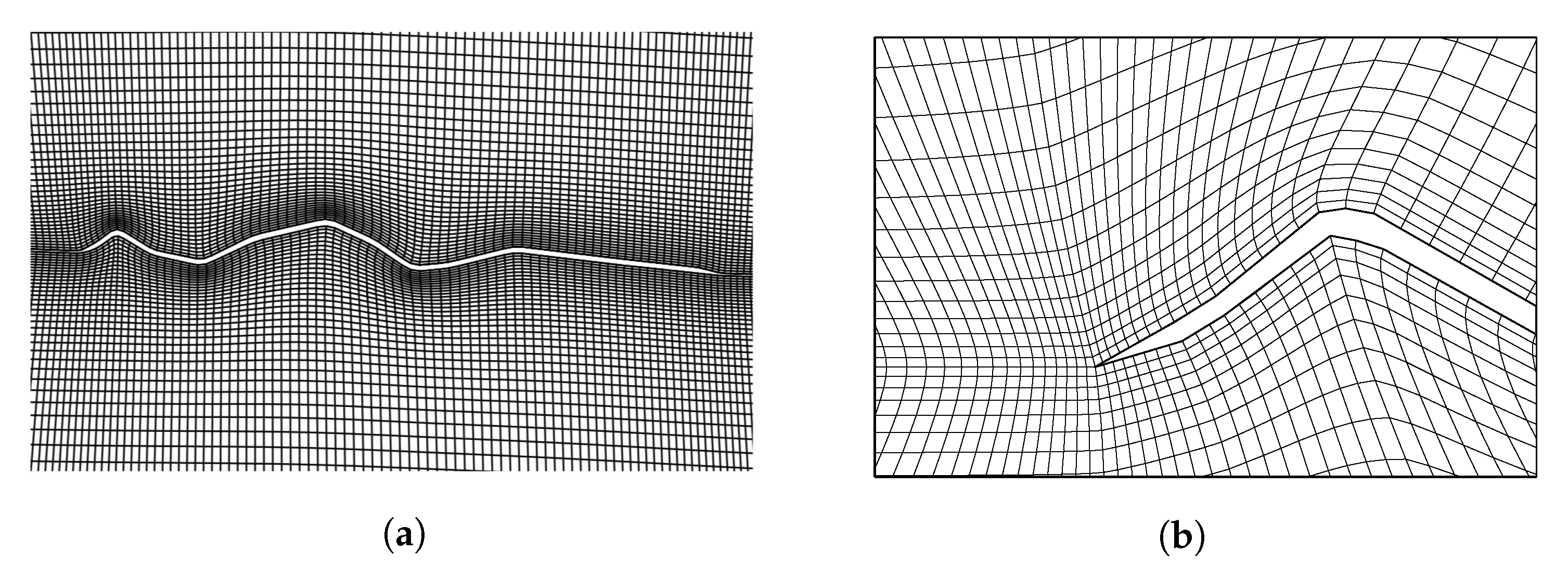
2. Numerical Method
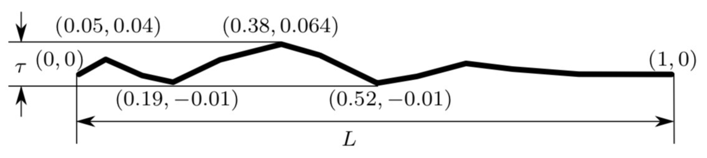
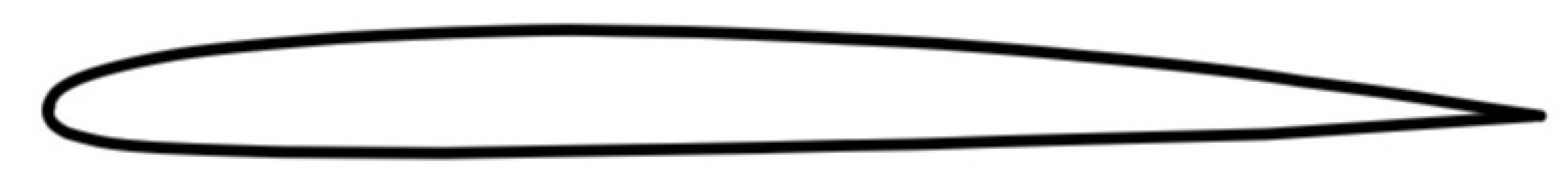
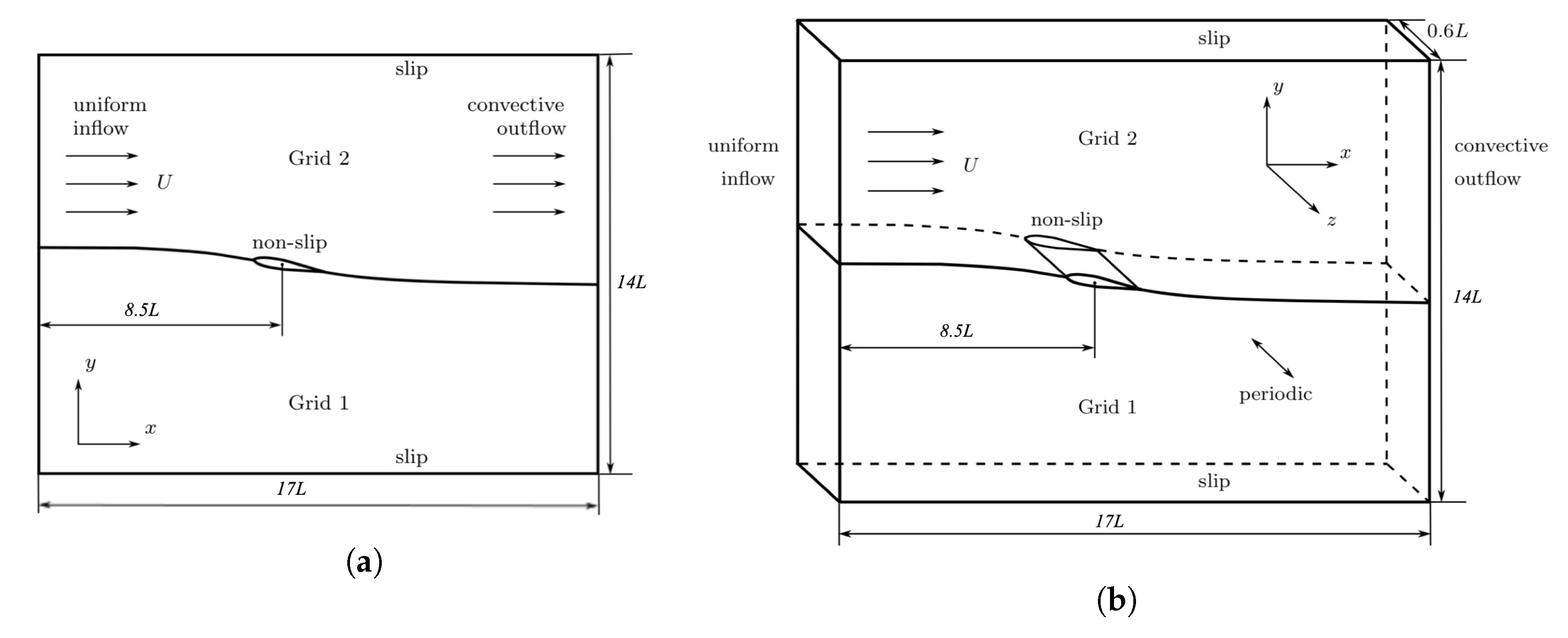
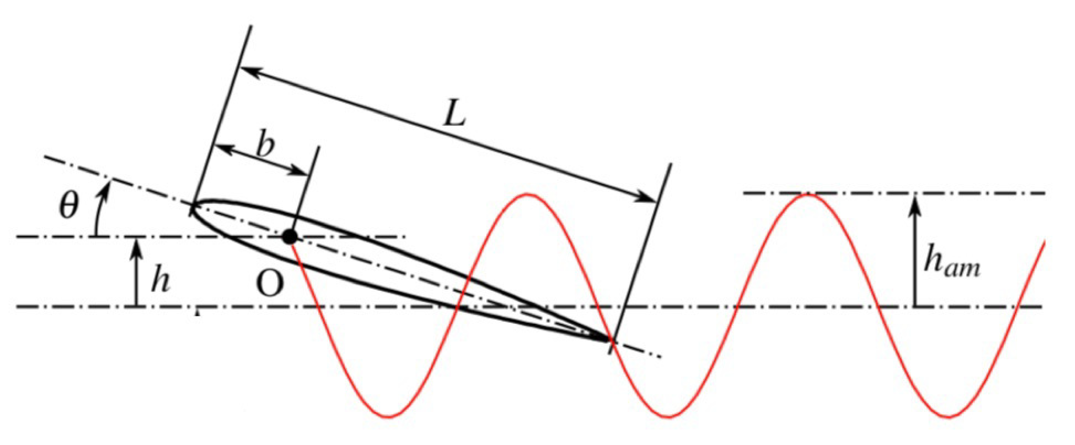
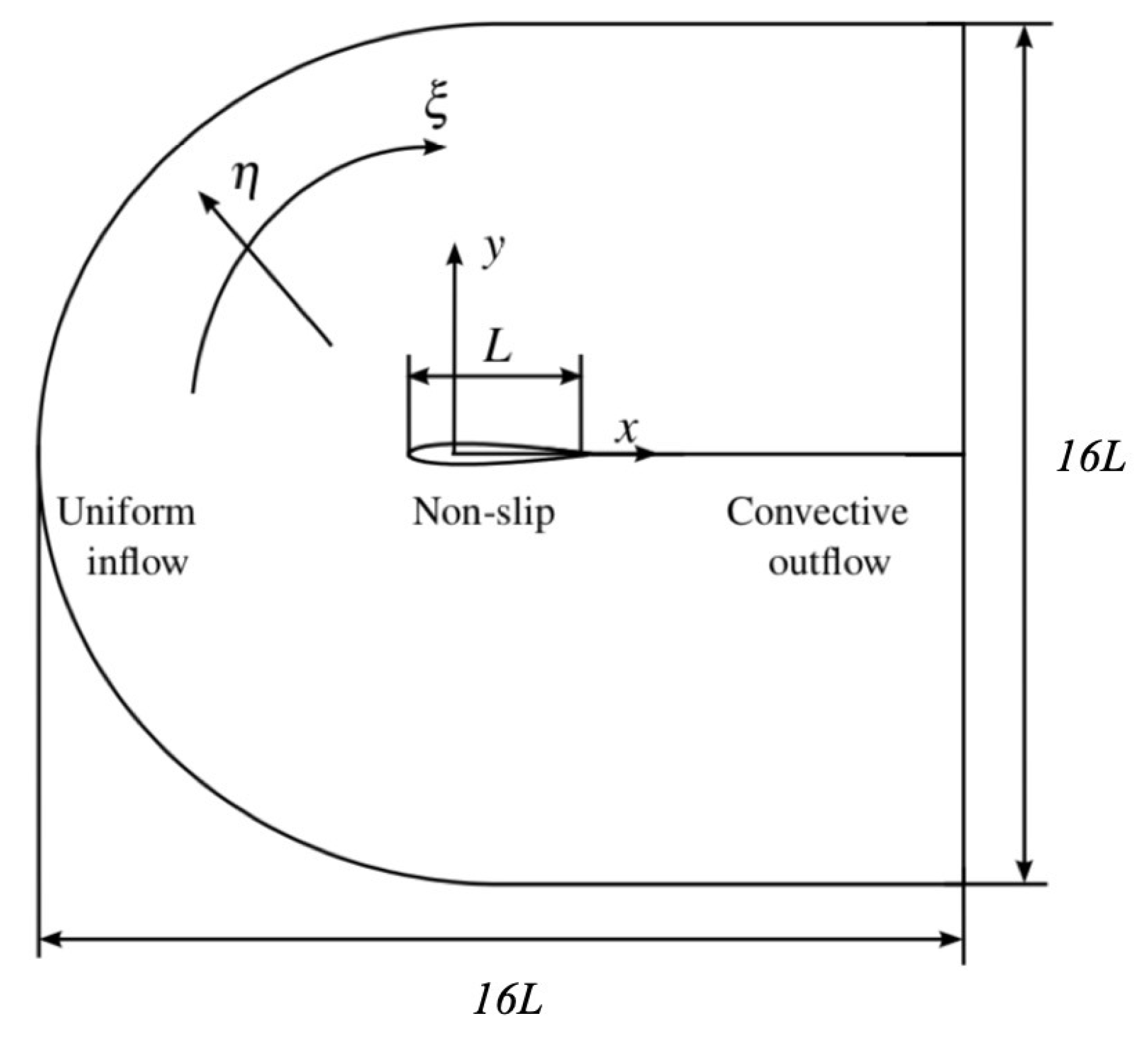
3. Computational Setup
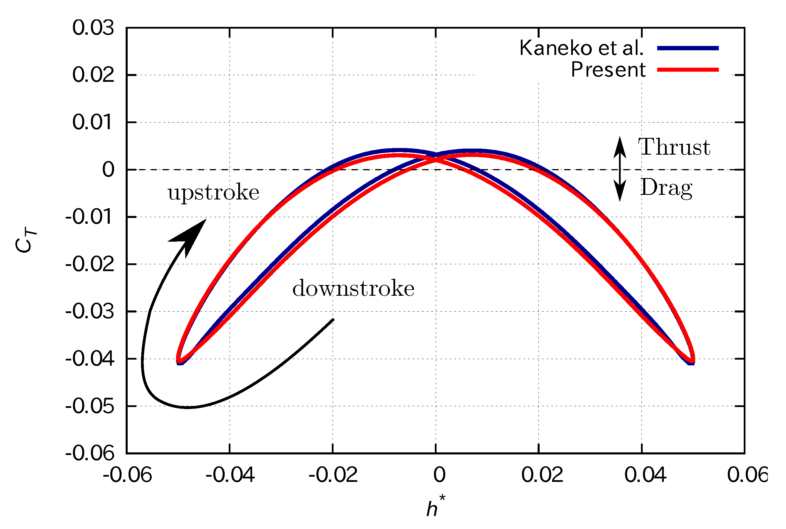
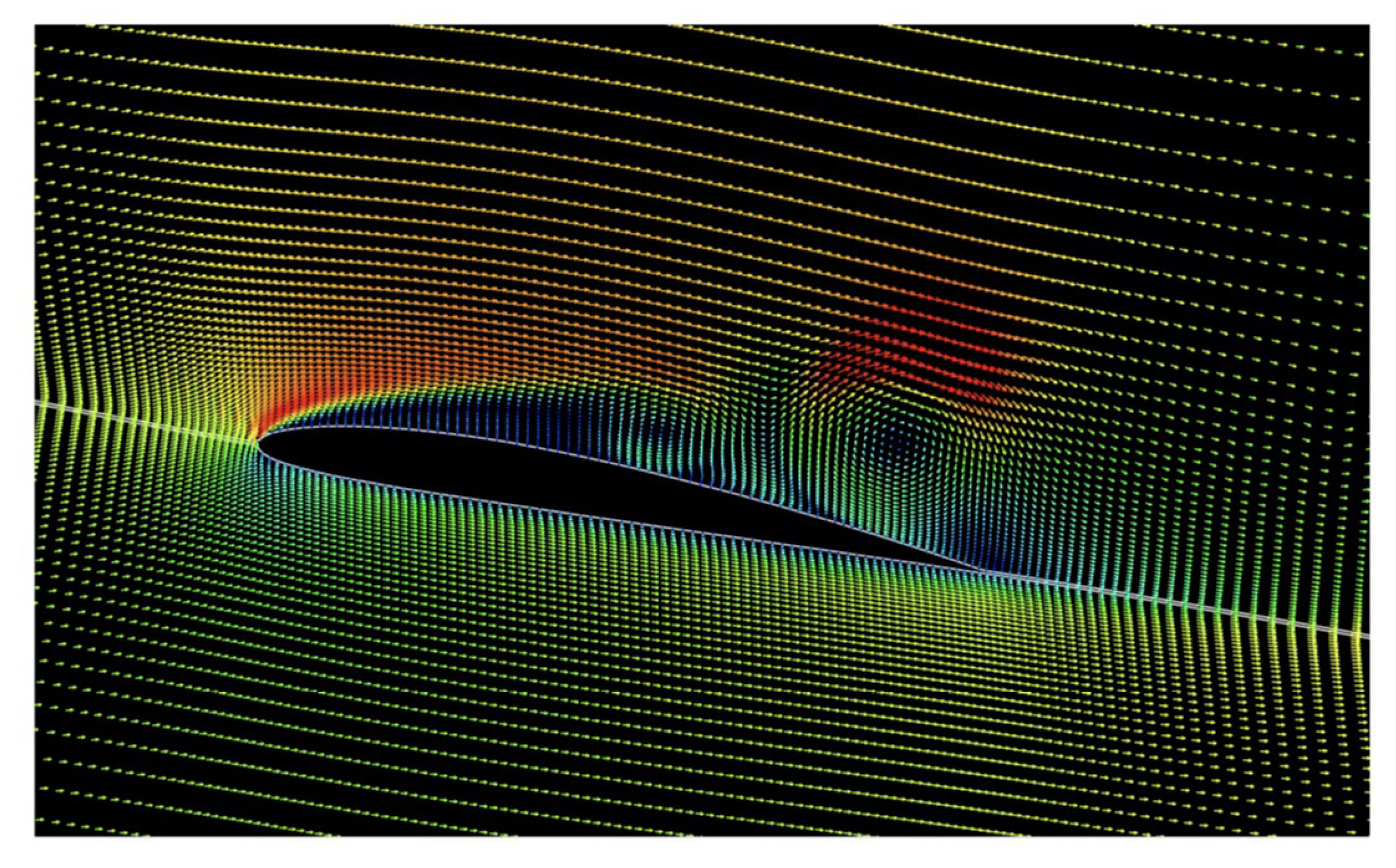
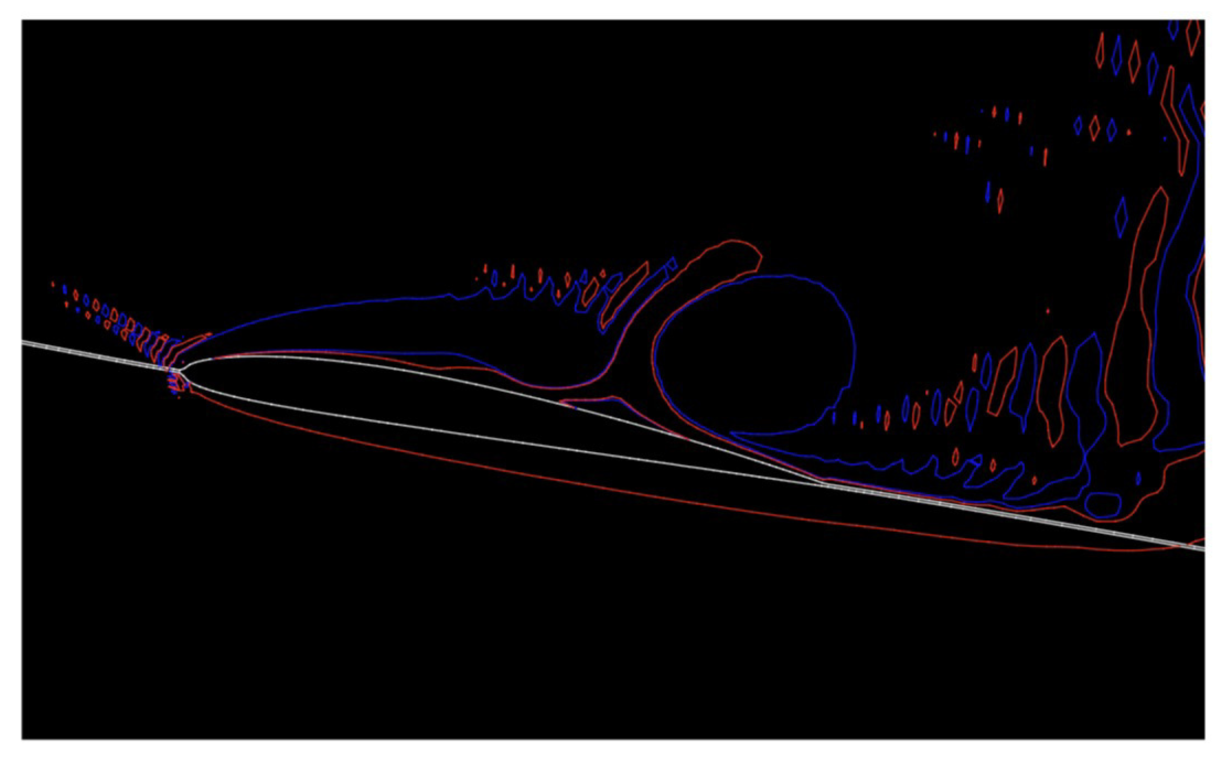
4. Validation Case
5. Results and Discussion
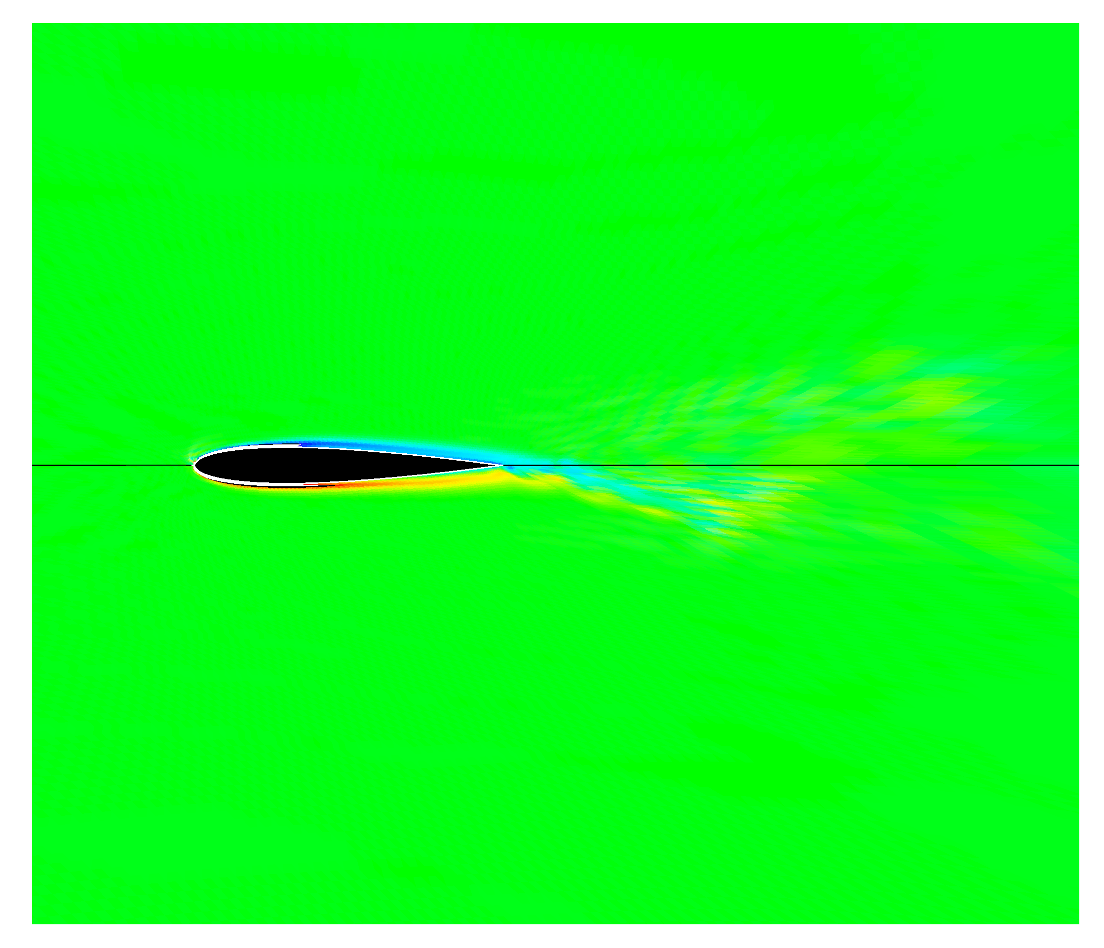
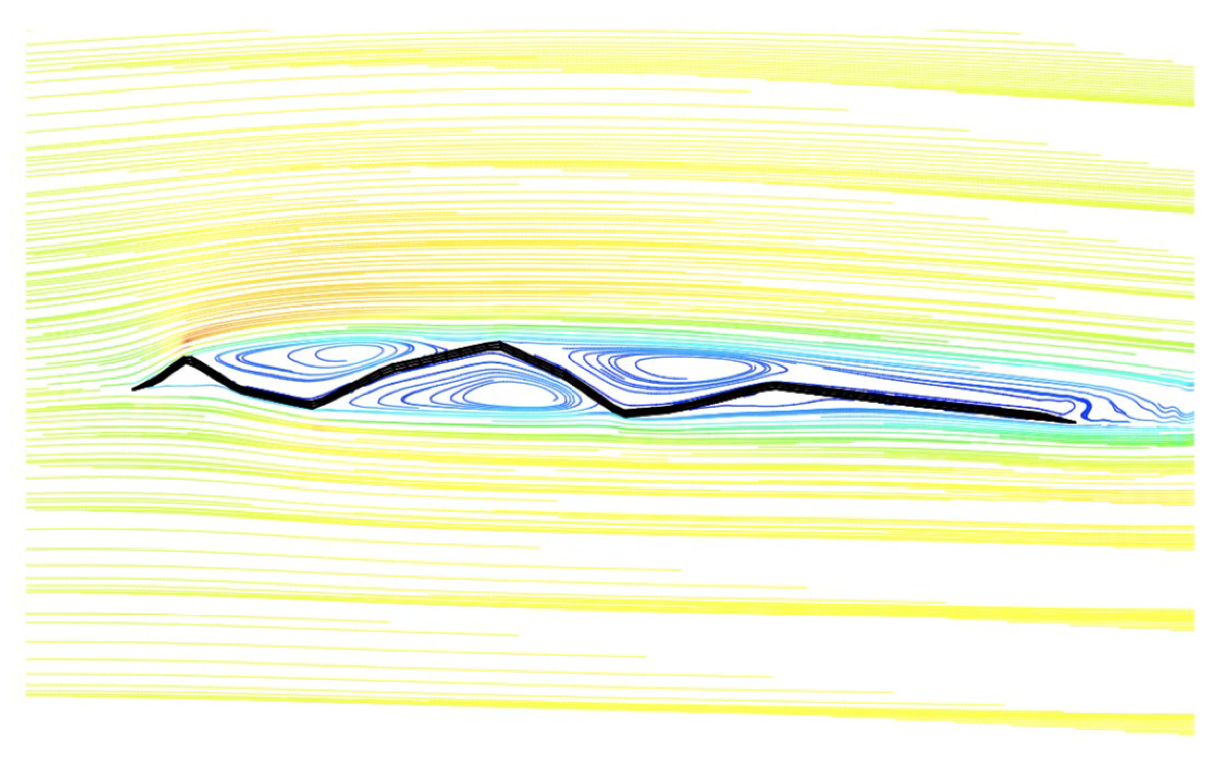
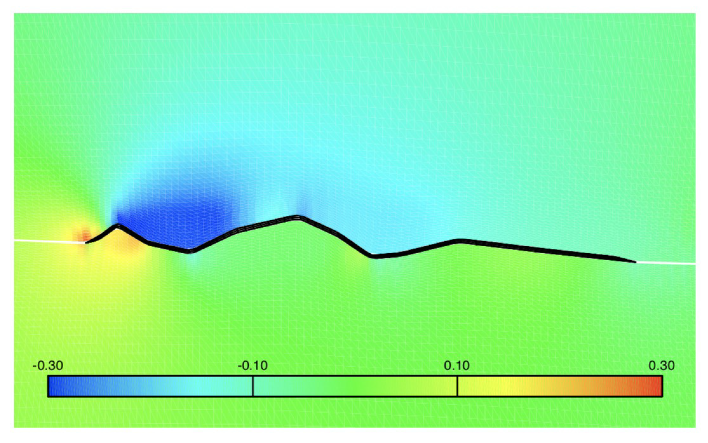
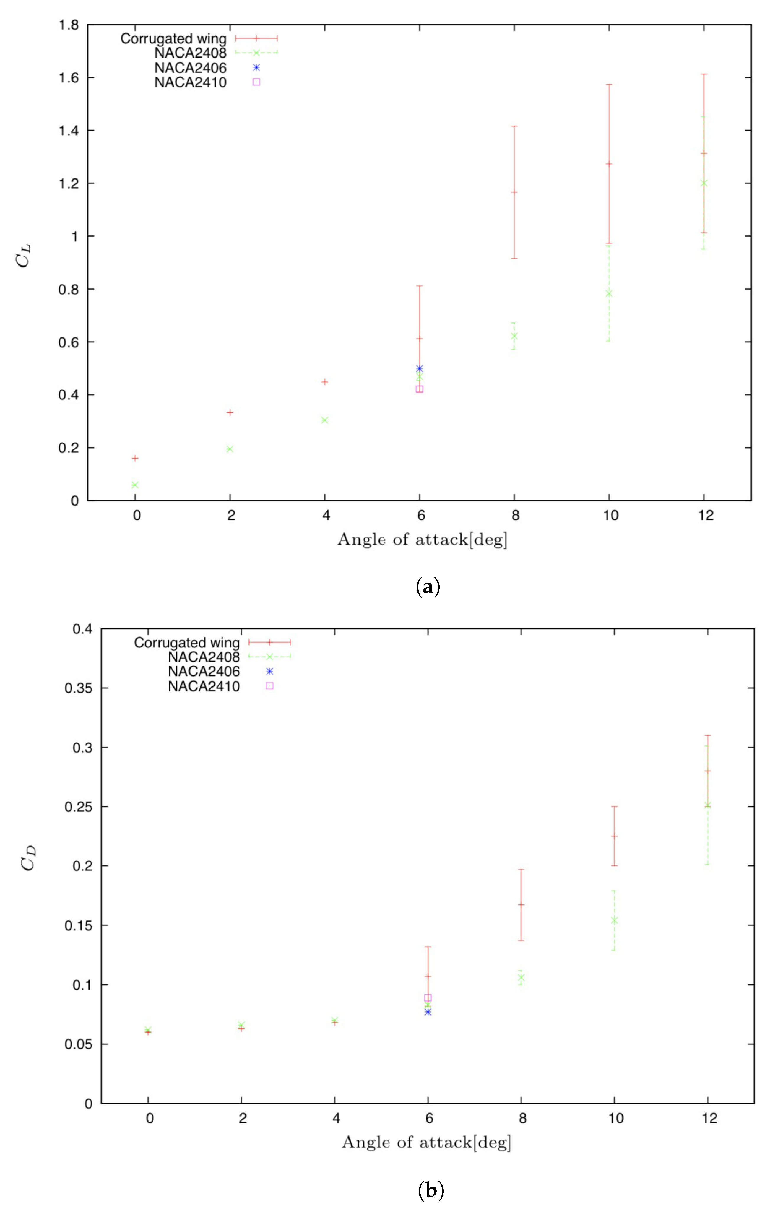
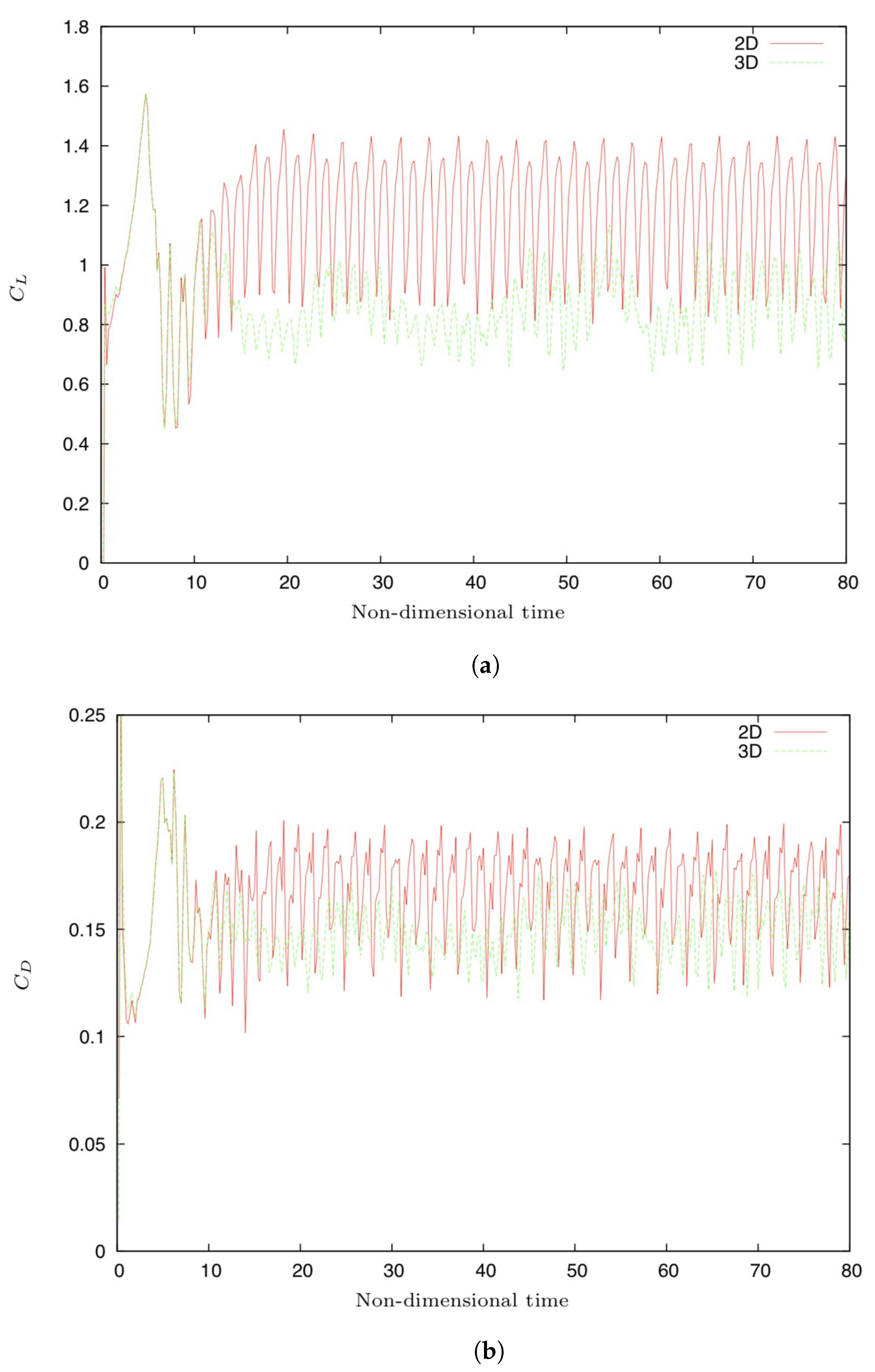
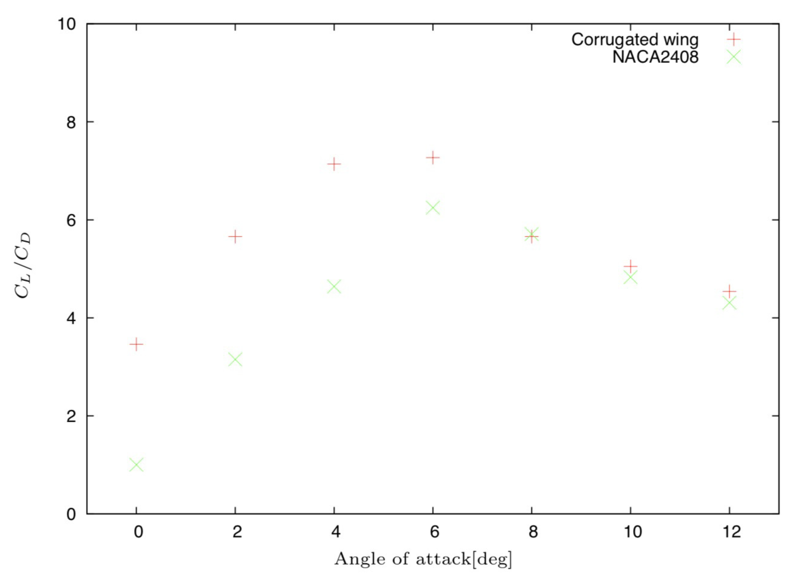
5.1. Aerodynamic Characteristics under Two-Dimensional Calculation
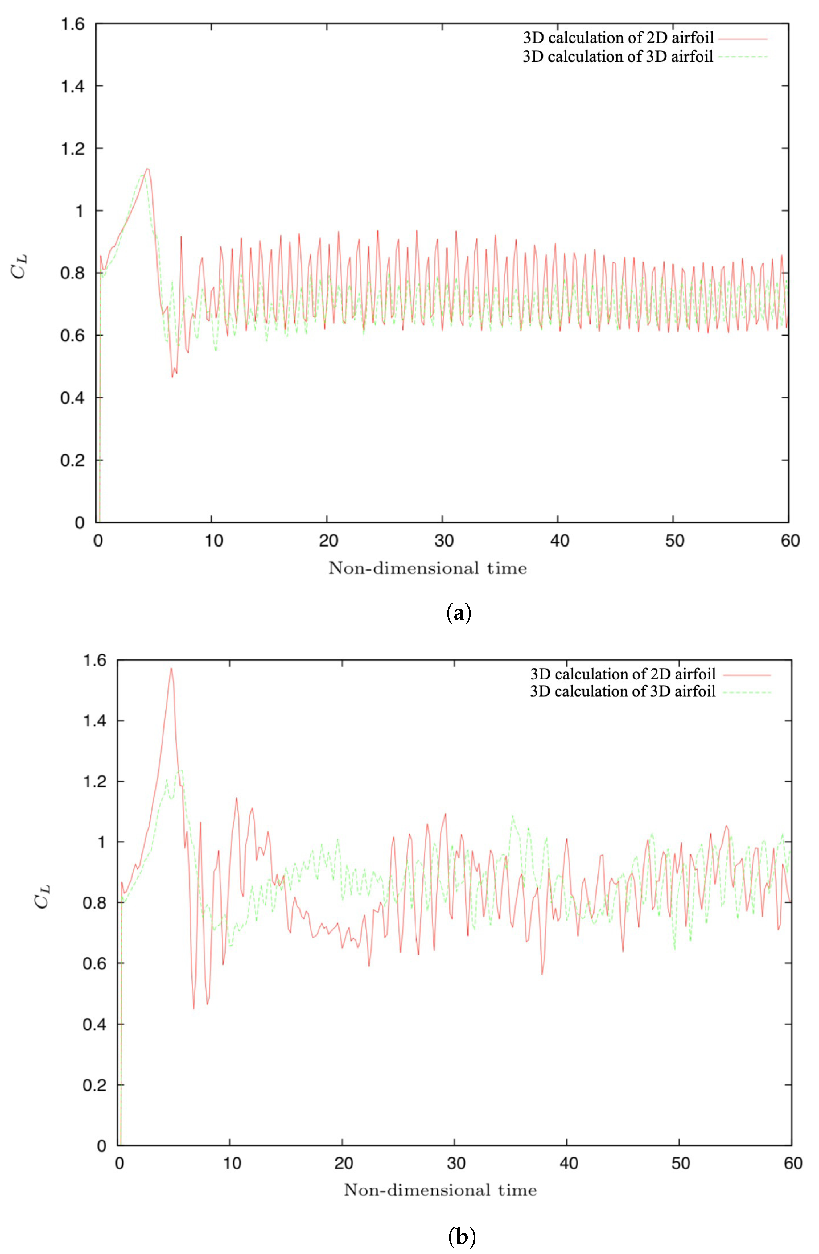
5.2. Aerodynamic Characteristics under Three-Dimensional Calculation
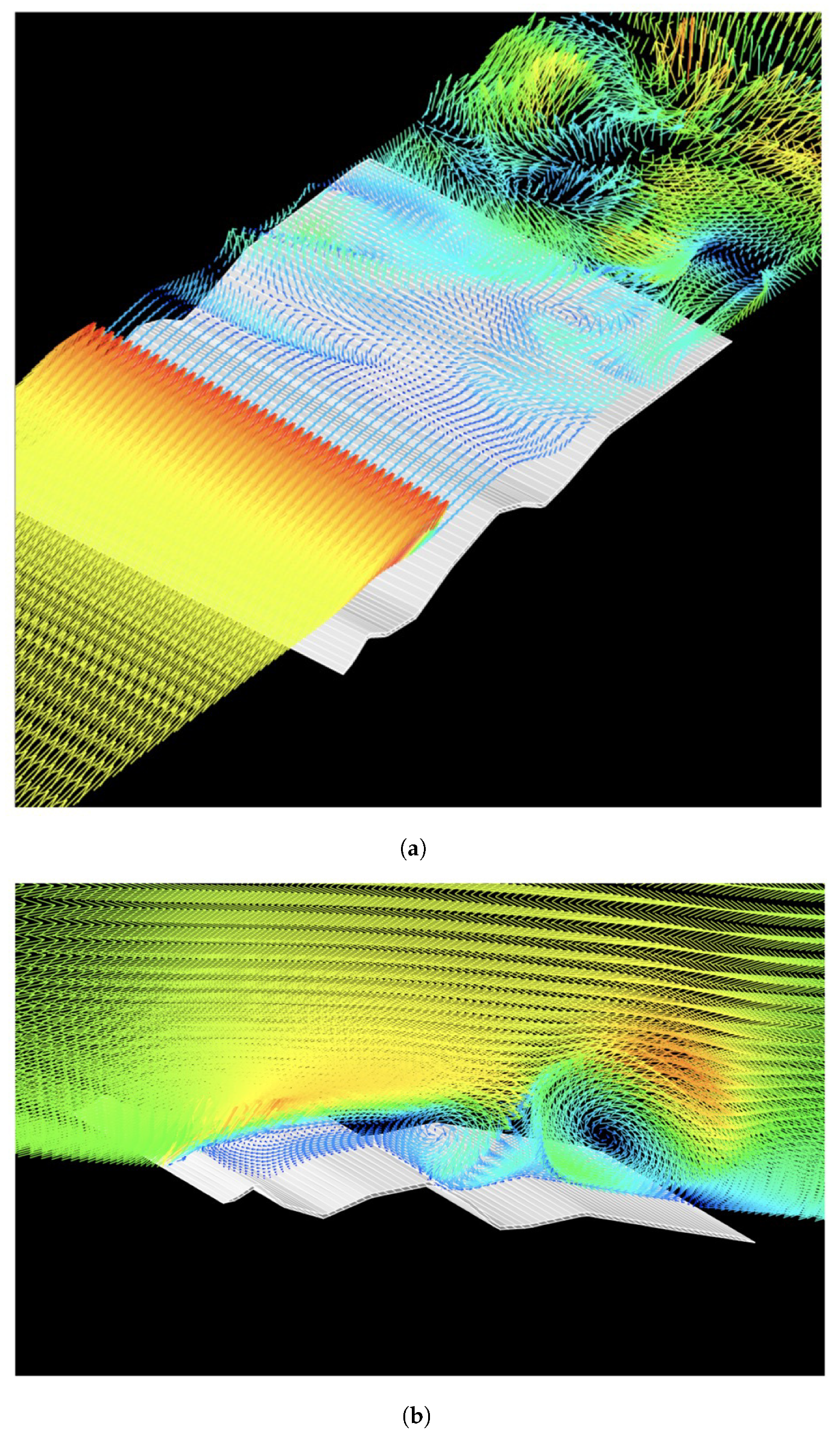
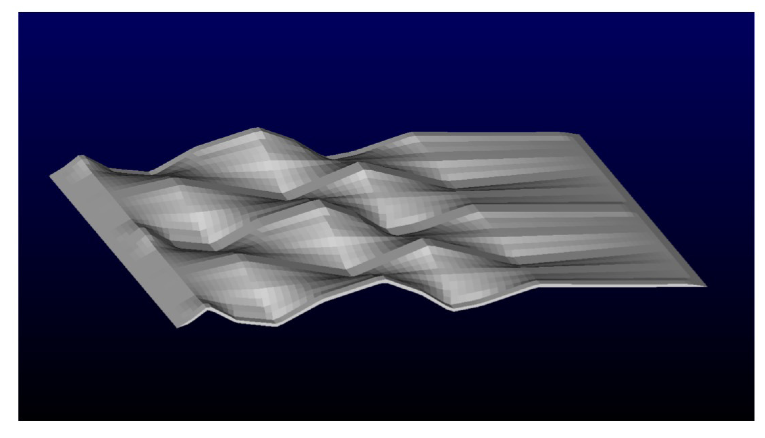
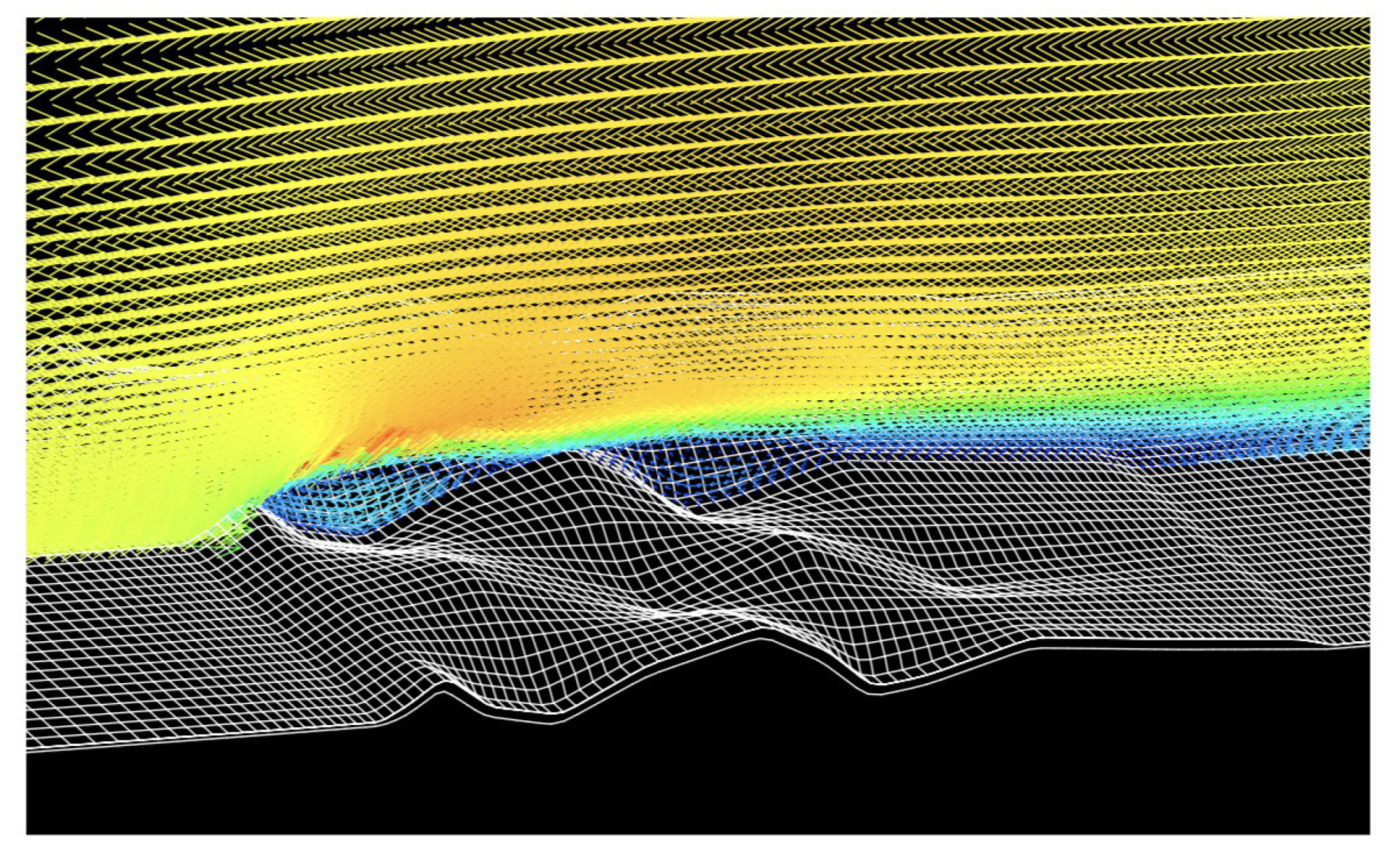
5.3. Aerodynamic Characteristics of Three-Dimensional Corrugated Airfoil under Three-Dimensional Calculation
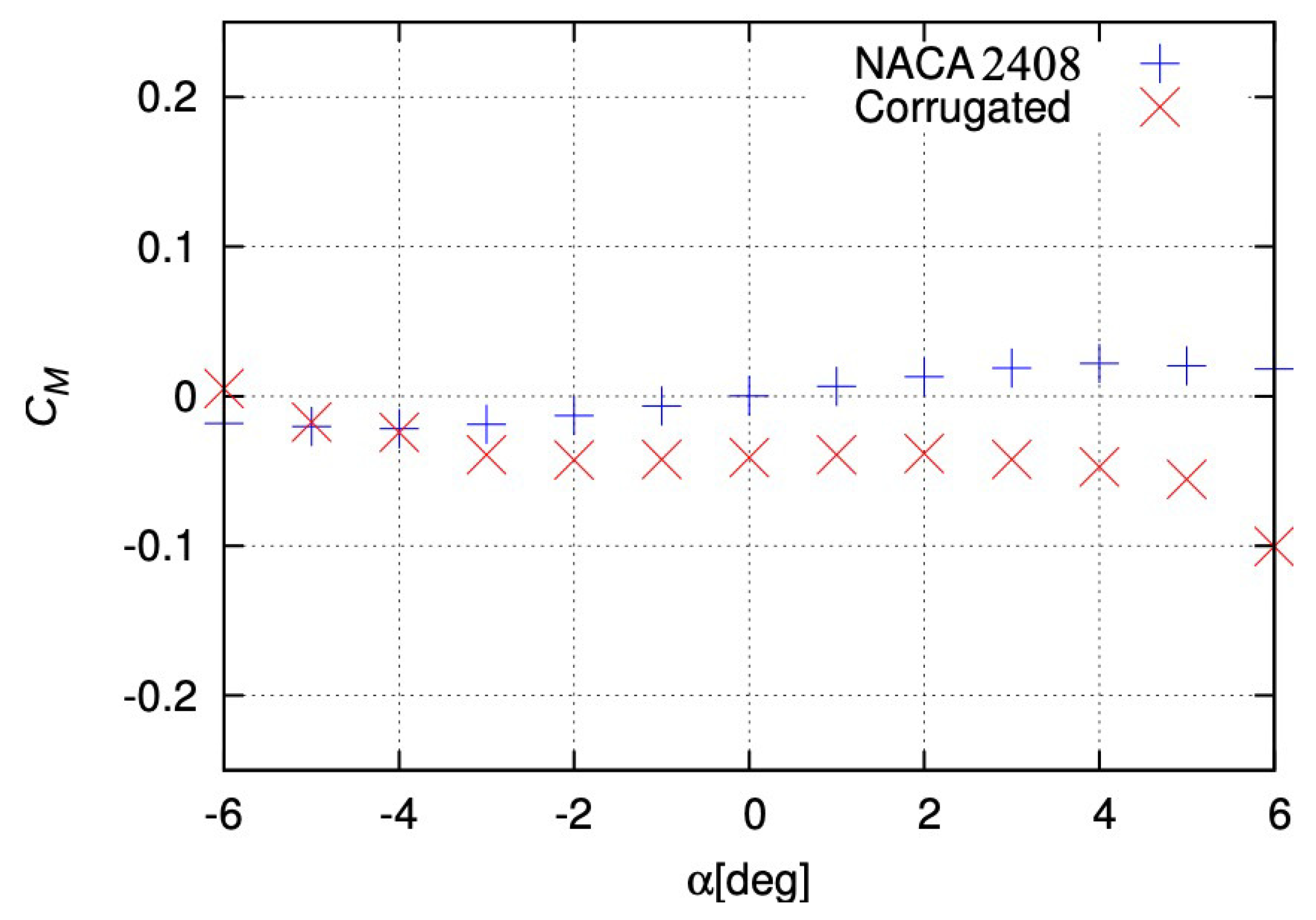
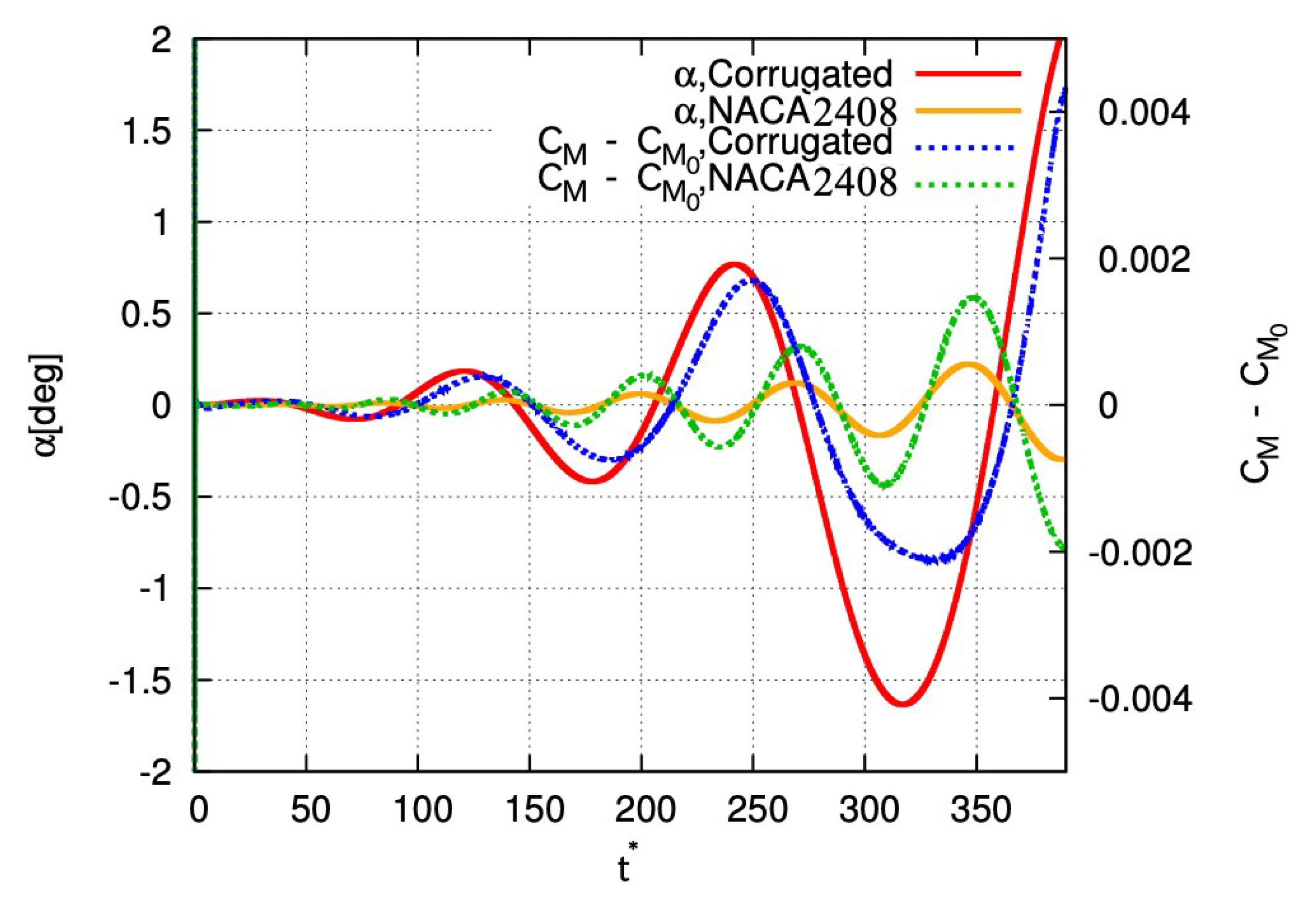
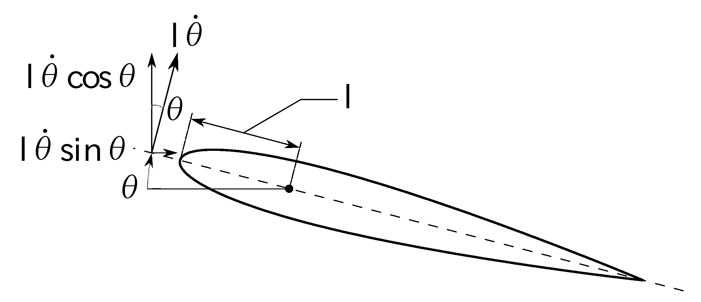
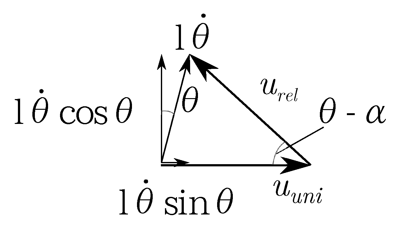
5.4. Hydrodynamic Moment and Attitude Stability
5.4.1. Fixed Angle of Attack
5.4.2. Angle of Attack Passively Changed by the Fluid Force
6. Conclusions
Author Contributions
Funding
Acknowledgments
Conflicts of Interest
Abbreviations
| 2D | two-dimensional |
| 3D | three-dimensional |
| MAVs | micro air vehicles |
| SOR | successive over-relaxation |
| UAVs | unmanned aerial vehicles |
References
- Mohiuddin, A.; Taha, T.; Zweiri, Y.; Gan, D. UAV payload transportation via RTDP based optimized velocity profiles. Energies 2019, 12, 3049. [Google Scholar] [CrossRef]
- Estevez, J.; Lopez-Guede, J.M.; Grana, M. Quasi-stationary state transportation of a hose with quadrotors. Robot. Auton. Syst. 2015, 63, 187–194. [Google Scholar] [CrossRef]
- Wall Street Journal. Google Drones Can Already Deliver You Coffee In Australia. Available online: https://www.youtube.com/watch?v=prhDrfUgpB0 (accessed on 6 April 2019).
- Stolaroff, J.K.; Samaras, C.; O’Neill, E.R.; Lubers, A.; Mitchell, A.S.; Ceperley, D. Energy use and life cycle greenhouse gas emissions of drones for commercial package delivery. Nat. Commun. 2018, 9, 409. [Google Scholar] [CrossRef] [PubMed]
- Carmichael, B.H. Low Reynolds Number Airfoil Survey, Volume 1; NASA CR-165803; NASA: Washington, DC, USA, 1981.
- Lissaman, P.B.S. Low-Reynolds-number airfoils. Annu. Rev. Fluid Mech. 1983, 15, 223–239. [Google Scholar] [CrossRef]
- Gad-el-Hak, M. Micro-air-vehicles: Can they be controlled better? J. Aircr. 2001, 38, 419–429. [Google Scholar] [CrossRef]
- Wakeling, J.M.; Ellington, C.P. Dragonfly flight. I. Gliding flight and steady-state aerodynamic forces. J. Exp. Biol. 1997, 200, 543–556. [Google Scholar] [PubMed]
- Kesel, A.B. Aerodynamic characteristics of dragonfly wing sections compared with technical aerofoils. J. Exp. Biol. 2000, 203, 3125–3135. [Google Scholar]
- Rees, C.J. Form and function in corrugated insect wings. Nature 1975, 256, 200–203. [Google Scholar] [CrossRef]
- Brodsky, A.K. The Evolution of Insect Flight; Oxford University Press: Oxford, UK, 1994. [Google Scholar]
- Rudolph, R. Aerodynamic properties of Libellula quadrimaculata L.(Anisoptera: Libellulidae), and the flow around smooth and corrugated wing section models during gliding flight. Odonatologica 1978, 7, 49–58. [Google Scholar]
- Okamoto, M.; Yasuda, K.; Azuma, A. Aerodynamic characteristics of the wings and body of a dragonfly. J. Exp. Biol. 1996, 199, 281–294. [Google Scholar]
- Luo, G.; Sun, M. The effects of corrugation and wing planform on the aerodynamic force production of sweeping model insect wings. Acta Mech. Sin. 2005, 21, 531–541. [Google Scholar] [CrossRef]
- Vargas, A.; Mittal, R.; Dong, H. A computational study of the aerodynamic performance of a dragonfly wing section in gliding flight. Bioinspir. Biomim. 2008, 3, 026004. [Google Scholar] [CrossRef] [PubMed] [Green Version]
- Murphy, J.T.; Hu, H. An experimental study of a bio-inspired corrugated airfoil for micro air vehicle applications. Exp. Fluids 2010, 49, 531–546. [Google Scholar] [CrossRef]
- Khan, M.D.; Padhy, C.; Nandish, M.; Rita, K. Computational Analysis of Bio-Inspired Corrugated Airfoil with Varying Corrugation Angle (16 February 2018). Available online: https://ssrn.com/abstract=3124809 (accessed on 22 October 2019).
- Uppu, S.P.; Manisha, D.; Devi, G.D.; Chengalwa, P.; Devi, B.V. Aerodynamic Analysis of a Dragonfly. J. Adv. Res. Fluid Mech. Therm. Sci. J. 2018, 1, 31–41. [Google Scholar]
- Mohamed, A.; Massey, K.; Watkins, S.; Clothier, R. The attitude control of fixed-wing MAVS in turbulent environments. Prog. Aerosp. Sci. 2014, 66, 37–48. [Google Scholar] [CrossRef]
- Orr, M.W.; Rasmussen, S.J.; Karni, E.D.; Blake, W.B. Framework for developing and evaluating MAV control algorithms in a realistic urban setting. In Proceedings of the IEEE 2005 American Control Conference, Portland, OR, USA, 8–10 June 2005; pp. 4096–4101. [Google Scholar]
- Galinski, C.E.Z.A.R.Y.; Zbikowski, R. Some problems of micro air vehicles development. Bull. Pol. Acad. Sci. Tech. Sci. 2007, 55, 91–98. [Google Scholar]
- Mohamed, A.; Clothier, R.; Watkins, S.; Sabatini, R.; Abdulrahim, M. Fixed-wing MAV attitude stability in atmospheric turbulence, part 1: Suitability of conventional sensors. Prog. Aerosp. Sci. 2014, 70, 69–82. [Google Scholar] [CrossRef]
- Chorin, A.J. A numerical method for solving incompressible viscous flow problems. J. Comput. Phys. 1967, 2, 12–26. [Google Scholar] [CrossRef]
- Tamura, A.; Kikuchi, K.; Takahashi, T. Residual cutting method for elliptic boundary value problems. J. Comput. Phys. 1997, 137, 247–264. [Google Scholar] [CrossRef]
- Kajishima, T.; Ohta, T.; Okazaki, K.; Miyake, Y. High-order finite-difference method for incompressible flows using collocated grid system. JSME Int. J. Ser. B Fluids Therm. Eng. 1998, 41, 830–839. [Google Scholar] [CrossRef]
- Ohta, T.; Kajishima, T. Analysis of non-steady separated turbulent flow in an asymmetric plane diffuser by direct numerical simulations. J. Fluid Sci. Technol. 2010, 5, 515–527. [Google Scholar] [CrossRef]
- Tang, H.; Lei, Y.; Fu, Y. Noise Reduction Mechanisms of an Airfoil with Trailing Edge Serrations at Low Mach Number. Appl. Sci. 2019, 9, 3784. [Google Scholar] [CrossRef]
- Obata, A.; Sinohara, S. Flow visualization study of the aerodynamics of modeled dragonfly wings. AIAA J. 2009, 47, 3043–3046. [Google Scholar] [CrossRef]
- Thompson, J.F.; Soni, B.K.; Weatherill, N.P. Handbook of Grid Generation; CRC Press: Boca Raton, FL, USA, 1998. [Google Scholar]
- Kaneko, Y.; Omori, K.; Kajishima, T. Numerical study on the aerodynamics of an airfoil moving close to an air-water interface. Trans. Jpn. Soc. Mech. Eng. 2016, 82, 16-00112. [Google Scholar]
- Anderson, J.M.; Streitlien, K.; Barrett, D.S.; Triantafyllou, M.S. Oscillating foils of high propulsive efficiency. J. Fluid Mech. 1998, 360, 41–72. [Google Scholar] [CrossRef] [Green Version]
- Nakae, Y.; Ohtake, T.; Muramatsu, A.; Motohashi, T. Three dimensionalization of the Flow Field around a NACA0012 Airfoil at Low Reynolds Numbers. J. Jpn. Soc. Aeronaut. Space Sci. 2011, 59, 244–251. [Google Scholar]
- Routh, E.J. A Treatise on the Stability of a Given State of Motion: Particularly Steady Motion; Macmillan and Company: Troon, Scotland, 1877. [Google Scholar]
- Hurwitz, A. Ueber die Bedingungen, unter welchen eine Gleichung nur Wurzeln mit negativen reellen Theilen besitzt. Mathem. Ann. 1895, 46, 273–284. [Google Scholar] [CrossRef]


| Case | Angle of Attack | ||||
|---|---|---|---|---|---|
| 2-D | 4000 | – | |||
| 3-D | 4000 | – |
| Angle of Attack | ||||||
|---|---|---|---|---|---|---|
| Case | |||||||
|---|---|---|---|---|---|---|---|
| Corrugated airfoil | |||||||
| NACA2408 airfoil |
| Dimensionless Time Delay | Corrugated | NACA2408 |
|---|---|---|
| Average | ||
| Coefficient of Variation |
© 2019 by the authors. Licensee MDPI, Basel, Switzerland. This article is an open access article distributed under the terms and conditions of the Creative Commons Attribution (CC BY) license (http://creativecommons.org/licenses/by/4.0/).
Share and Cite
Tang, H.; Lei, Y.; Li, X.; Fu, Y. Numerical Investigation of the Aerodynamic Characteristics and Attitude Stability of a Bio-Inspired Corrugated Airfoil for MAV or UAV Applications. Energies 2019, 12, 4021. https://doi.org/10.3390/en12204021
Tang H, Lei Y, Li X, Fu Y. Numerical Investigation of the Aerodynamic Characteristics and Attitude Stability of a Bio-Inspired Corrugated Airfoil for MAV or UAV Applications. Energies. 2019; 12(20):4021. https://doi.org/10.3390/en12204021
Chicago/Turabian StyleTang, Hui, Yulong Lei, Xingzhong Li, and Yao Fu. 2019. "Numerical Investigation of the Aerodynamic Characteristics and Attitude Stability of a Bio-Inspired Corrugated Airfoil for MAV or UAV Applications" Energies 12, no. 20: 4021. https://doi.org/10.3390/en12204021