Dynamic Modeling and Preliminary Performance Analysis of a New Solar Thermal Reverse Osmosis Desalination Process

Abstract

Reverse osmosis (RO) is a desalination technique that is commonly preferred because of its low energy consumption. In this paper, an innovative, thermally powered RO desalination process is presented. This new thermo-hydraulic process uses solar thermal energy in order to realize the pressurization of the saltwater beyond its osmotic pressure to allow its desalination. This pressurization is enabled thanks to a piston or a membrane set in motion in a reservoir by a working fluid that follows a thermodynamic cycle similar to an Organic Rankine Cycle. In this cycle, the evaporator is heated by low-grade heat, such as the one delivered by flat-plate solar collectors, while the condenser is cooled by the saltwater to be treated. Such an installation, designed for small-scale (1 to 10 m³·day⁻¹) brackish water desalination, should enable an average daily production of 500 L of drinkable water per m² of solar collectors with a specific thermal energy consumption of about 6 kWh_th·m⁻³. A dynamic modeling of the whole process has been developed in order to study its dynamic cyclic operating behavior under variable solar thermal power, to optimize its design, and to maximize its performances. This paper presents the preliminary performance results of such a solar-driven desalination process.

1. Introduction

Growth of the demand in seawater and brackish water desalination over the past few years has been motivated by increasing water stress in an increasing number of countries. Even if a major part of desalination systems is powered by fossil energies, desalination systems driven by renewable energies are now well-known and available on the market. Solar desalination is particularly interesting, considering how the most water-lacking areas are coastal and have an important sun resource.

Solar-driven desalination can be led in two different ways: distillation or membrane separation. In solar distillation systems, the water is evaporated by the solar heat. The most current distillation-based technologies are the multi-effect distillation (MED) and the multi-stage flash distillation (MSF). Those processes have a total specific primary energy consumption (SEC) commonly ranging between 30 and 80 kWh per cubic meter of produced clean water [1]. The consumed energy is, in this case, mostly thermal, but some processes include mechanical circulation or compression devices. In this case, the total primary energy can be assessed by taking into account an energy equivalent of mechanical energy to thermal energy, of which ratio is often taken to be approximately 3 kWh_th/kWh_el.

Membranes-based desalination consists in separating the salt from the water through a semi-permeable membrane. The most-implemented membrane separation processes are electrodialysis and reverse osmosis (RO). In electrodialysis processes, the salt is drained through an ion-selective membrane by way of two electrodes submitted to electrical potential. This process needs electrical energy to operate, and leads to an energy consumption lower than 2 kWh_elec·m⁻³. The process is more appropriate for brackish water desalination with a salinity below 2 g·L⁻¹ [2,3].

Reverse osmosis is a membrane separation technique which is widely used for desalination and food applications. RO desalination represents 65% of worldwide desalination systems [4], mainly for its high performance and relatively low production cost. In RO processes, the pressurized feed water flows through a semi-permeable membrane which retains the salt ions and only lets water go through. In order to make this permeation possible, the feed water has to be pressurized beyond its osmotic pressure, which depends on the salt concentration and water temperature. The RO technology leads to specific energy consumptions ranging from 2 to 10 kWh_mec·m⁻³ [5], and depends on the water salinity (from 2 to 40 g·L⁻¹) and temperature. This low energy consumption is obtained by recovering the hydraulic energy of the highly pressurized concentrated water at the membrane output by means of energy recovery devices, such as turbines or pressure exchangers. Distillation-based systems are easier to set up, but their energy consumptions are higher than membrane-based technologies. Membranes-based desalination enables low energy consumption in comparison to distillation processes, but they have some major operating issues, such as membrane deterioration or fouling, that can lead to higher operating costs. Nevertheless, reverse osmosis is an interesting technology because of its low energy needs and its potential to be implemented at a wider scale [6]. Solar photovoltaic-driven RO processes (PV-RO) have been widely developed nowadays, thanks to the modularity of these two components and the price drop of photovoltaics panels [7]. Recently, more interest has been brought to battery-less PV-RO that is more eco-friendly and has the benefit of lower investment costs [8,9]. Nevertheless, exploiting solar energy via photovoltaic panels in order to produce electricity, later converted into hydraulic energy, implies the use of high-pressure pumps and associated control devices that leads to important losses of efficiency [10]. These losses are mostly due to successive energy conversion. Furthermore, intermittent operation has been proven to increase biofouling because of the water non-circulation times [11]. Solar heat-driven RO-based systems obtained by coupling a thermal solar collector to a di-thermal power cycle and a RO unit could be an interesting solution to reduce energy conversion losses, and thus to obtain better energy efficiencies [12,13]. Manolakos et al. studied and experimented with a solar-driven RO desalination unit by implementing an Organic Rankine Cycle (ORC) [14]. They obtained relatively interesting performances despite the losses from its long energy conversion chain composed from expanders and pumps. They showed that solar thermal-driven reverse osmosis could be a competitive desalination technique. To avoid this kind of loss, another ORC-RO process was developed by Igobo et al. [15]. In their process, the expansion energy is directly transmitted to the feed water by a cylinder, and it also has very low mechanical energy consumption. Another similar process was developed by Nihill et al. in 2018, where they coupled a thermal water pump to a RO membrane [16]. In their study, the working fluid expansion is also realized in a cylinder with a mobile piston. In this process, the cylinder, which is directly heated by a heat exchanger, acts as an evaporator. This process allows desalination of the brackish water with a salinity of about 1.1 g·L⁻¹ by reaching 2.2 bars of pressure. However, this work is still under development, and shows high thermal energy consumption since it presents high thermodynamic irreversibilities due to pressurization and depressurization phases in the cylinder, and also does not include any mechanical energy recovery devices yet on the brine.

With the same guiding idea, an innovative thermo-hydraulic process is described and investigated in this paper. This process also enables the direct use of the expansion work of a fluid that follows a thermodynamic engine cycle, in order to pressurize the saline water in the RO unit. Importantly, this solution enables the reduction of energy conversion losses during the mechanical work conversion, and improves the efficiency of the global process. The process implements simple hydraulic and thermal components in order to be cost-effective, as well as easy to maintain and to operate. It can be powered by low-grade heat, such as solar heat provided by common flat-plate solar collectors. With these features, the process is able to operate in off-grid, remote areas. However, such a process generates a highly dynamic evolution of the pressure that is imposed to the RO membrane due to the sun irradiation variability and the cyclic behavior of the thermo-hydraulic engine. This pressure evolution consists in cyclic changes of pressure lasting a few minutes, where each cycle is characterized by a step change in pressure, followed by a plateau, and then a progressive decrease. The impact of these unsteady operating conditions on the RO unit performance has to be evaluated, and requires precise modelling that enables assessment of the effects of this pressure variation on the RO membrane performance.

The impact of dynamic applied pressure on the RO membrane, which affects its performances, is not yet well-known. Only a few studies on RO process operations in transient running conditions have been led, and these concluded only that the membrane performance was significantly affected by these dynamic operating conditions. 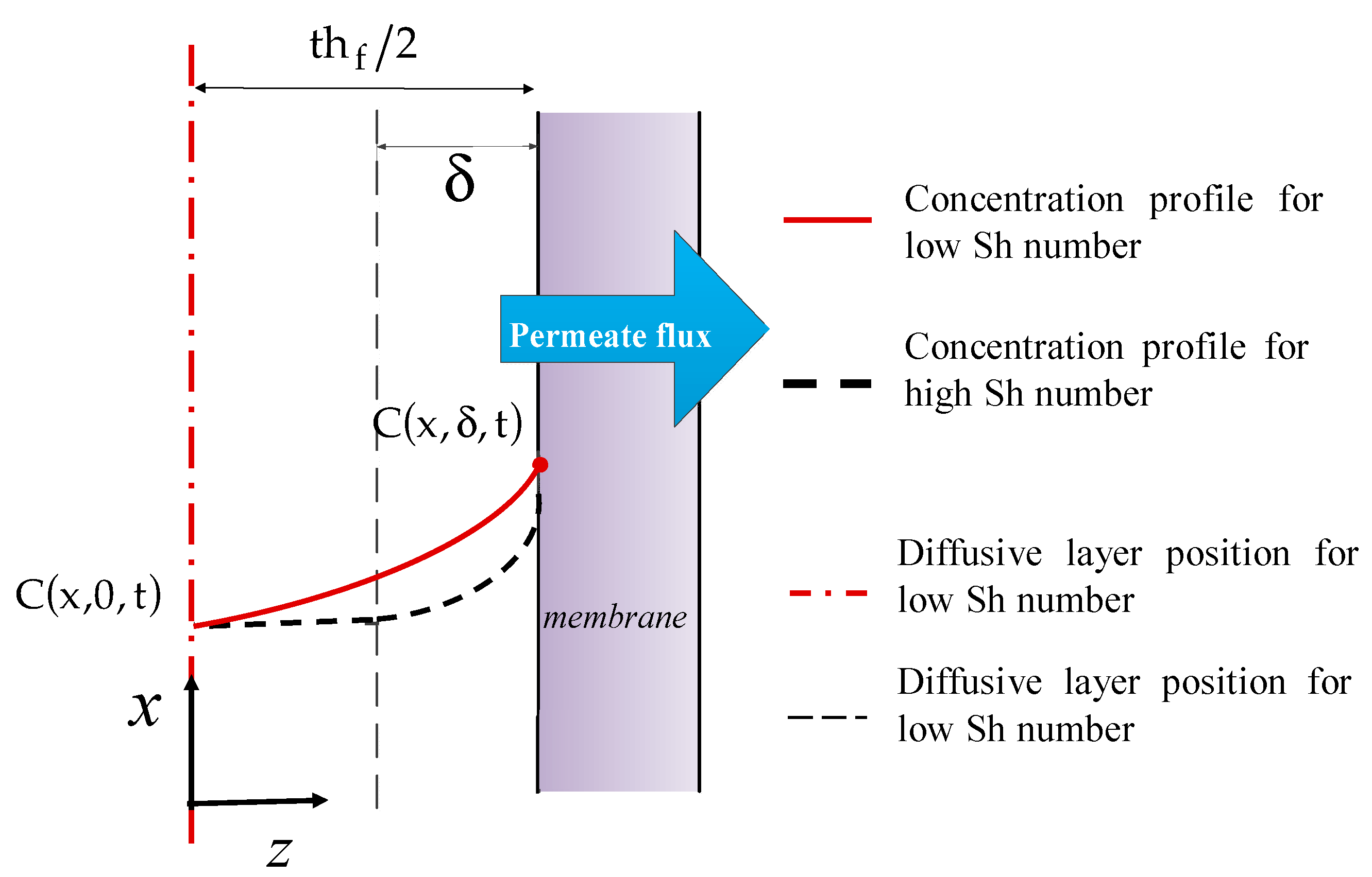Several linked phenomena have been reported, such as membrane compaction [17], higher salt accumulation at the membrane wall, and development of a greater diffusive layer in the feed water channel [18]. The latter phenomenon, called polarization, is well-known when a constant pressure is applied [19]. Yet, studies treating it in dynamic running conditions are not enough to predict the influence of dynamic pressure constraints, which are characteristic of the process studied in this paper.

Some studies have been led on RO processes operating under variable pressure constraints for several applications, such as photovoltaic-powered RO [17] or wastewater treatment [20]. They showed that dynamic running conditions have an impact on the salt concentration profile at the membrane wall which affects the permeation rate. Different kinds of transient modeling have been developed mainly with the assumption of a stationary diffusive layer that is established according to the well-known film theory. Rodgers et al. [21] developed dynamic modeling, and led experiments on an ultrafiltration process with a membrane submitted to pressure pulses. They studied the influence of these pressure pulses on polarization effects, and showed that short pulses of negative transmembrane pressure may increase the permeate flux and minimize the polarization effects. Kim et al. [22] compared the film theory results obtained by an analytical model and a two-dimensional numerical convection–diffusion model. This study, which has been experimentally validated, showed the relevance of the film theory model for steady working conditions. A dynamic model for tubular membranes was also introduced by Ali et al. [23] using a mathematical approach, and showed that a high step-change of the feed mass flow rate does impact the RO membrane behavior significantly. Besides these modeling studies, more practical researches have been made on RO desalination driven by unstable renewable energy sources. Cheddie et al. [24] studied a RO process powered by wave energy, and introduced dynamic modeling of the RO unit. They also showed that a periodic applied pressure may minimize the polarization effects and enhance the performances. Such works suggests that dynamic running conditions impact on RO membrane performances, and the membrane behavior needs to be modeled in a dynamic way in order to assess these impacts.

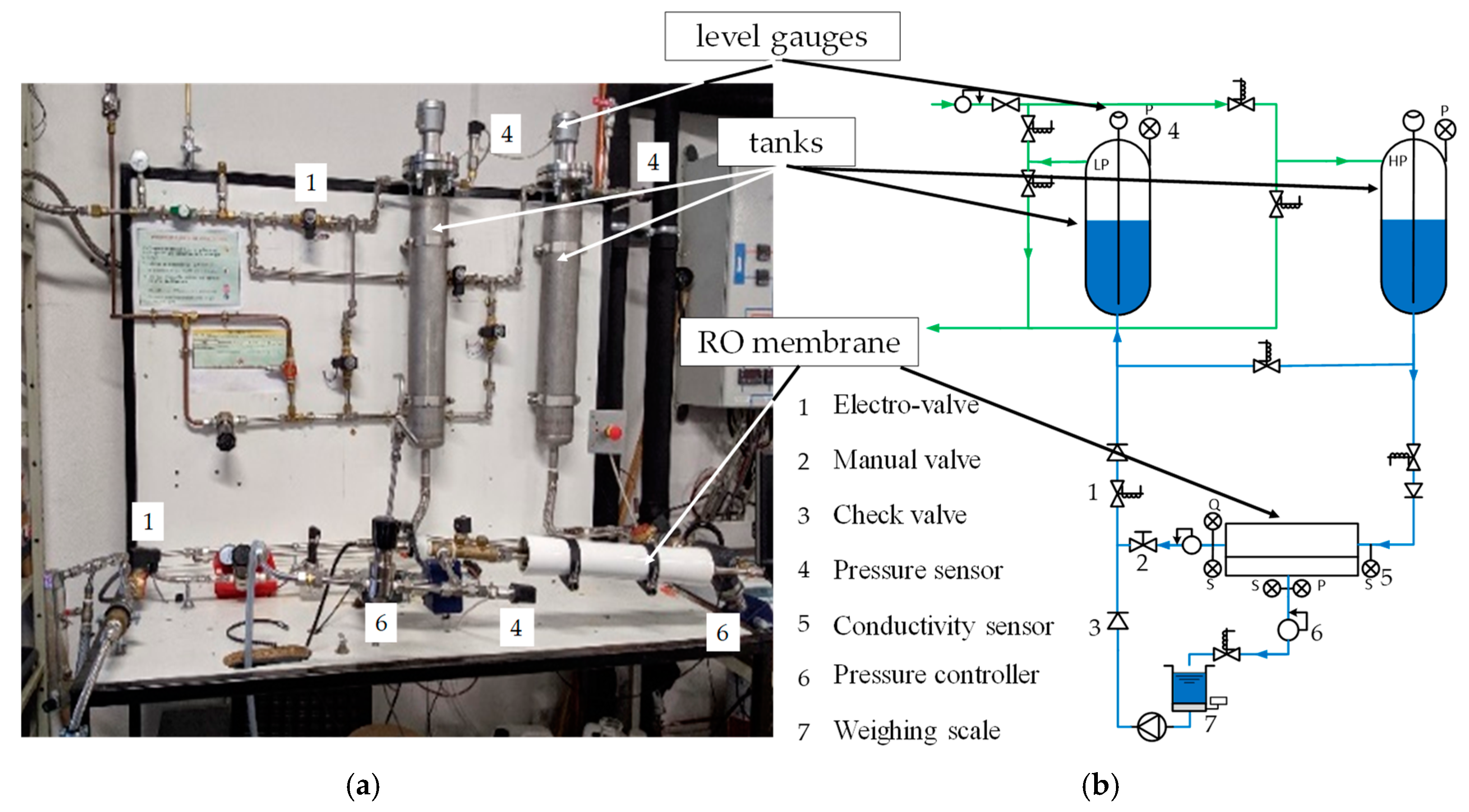
In this paper, a new solar heat-driven RO desalination process is described, and a dynamic modelling of the whole process is developed. In order to take the impacts of the cyclic pressure changes applied to the membrane into account, a 2D dynamic modelling of RO membrane is implemented. This membrane modelling enables a better understanding of the dynamic establishment of the polarization layer. An experimental study has also been carried out on a test bench designed for brackish water desalination under variable pressure evolutions and controlled mass flow rates of the brine in order to allow for a comparison with model results. Experimental data obtained with steady pressure tests are used to identify the parameter of the dynamic model. The experimental results obtained under dynamic operating tests are compared to numerical results in order to validate the dynamic modelling. Simulations of the whole process have been performed to study its dynamic behavior and analyze its performances.

2. Description of the Thermo-Hydraulic Desalination Process

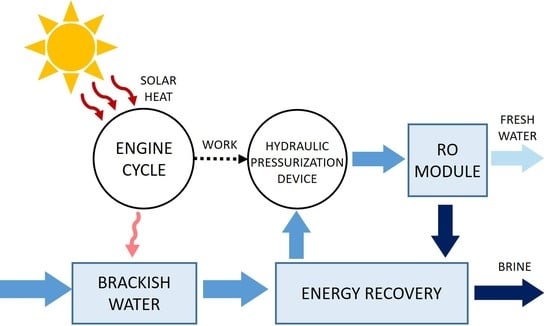
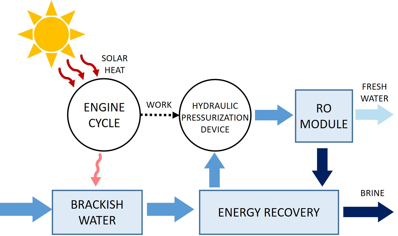
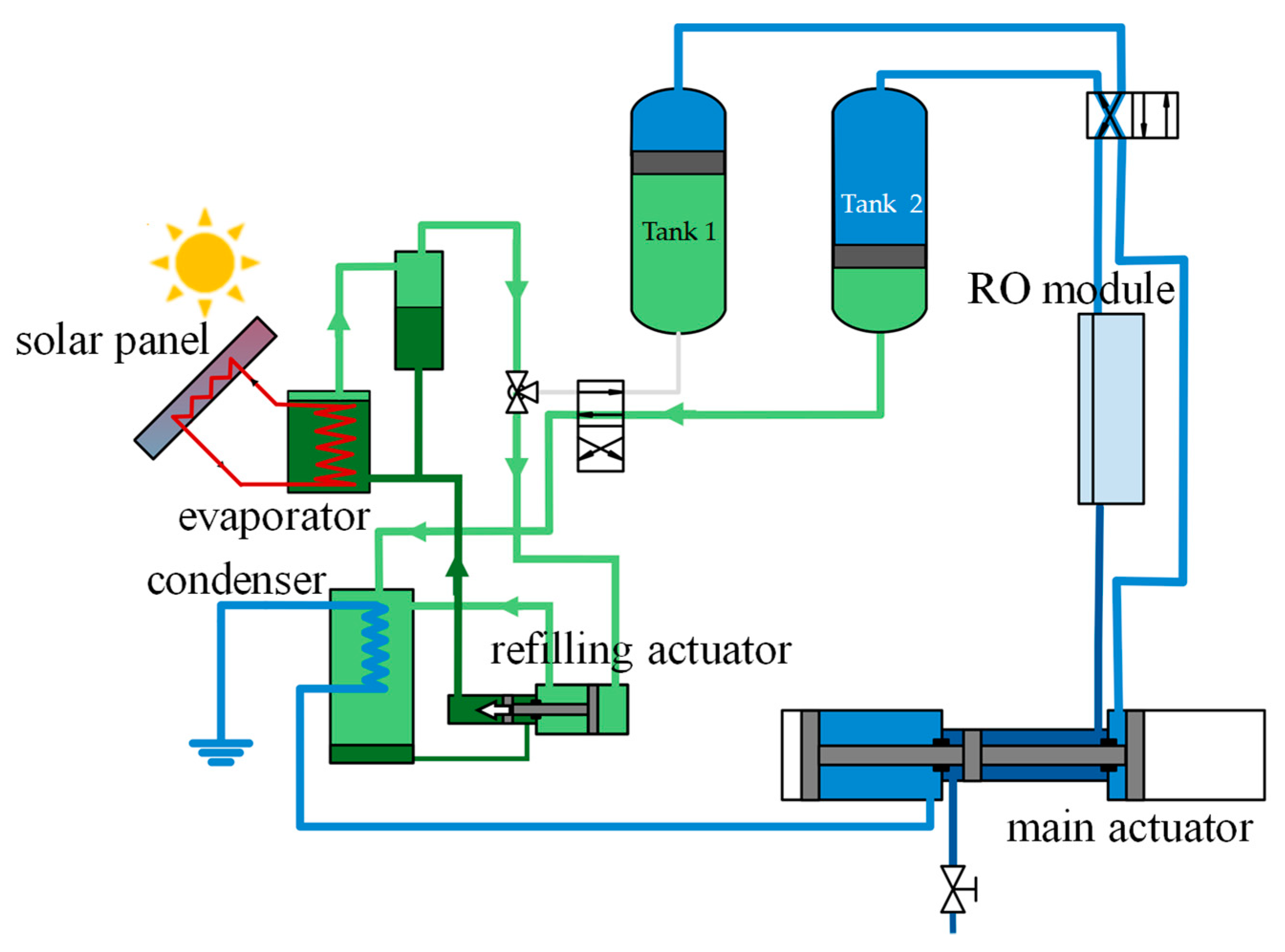
The thermo-hydraulic desalination process is described Figure 1. It results from a direct coupling of a solar-powered, Rankine-like engine cycle with a RO module.

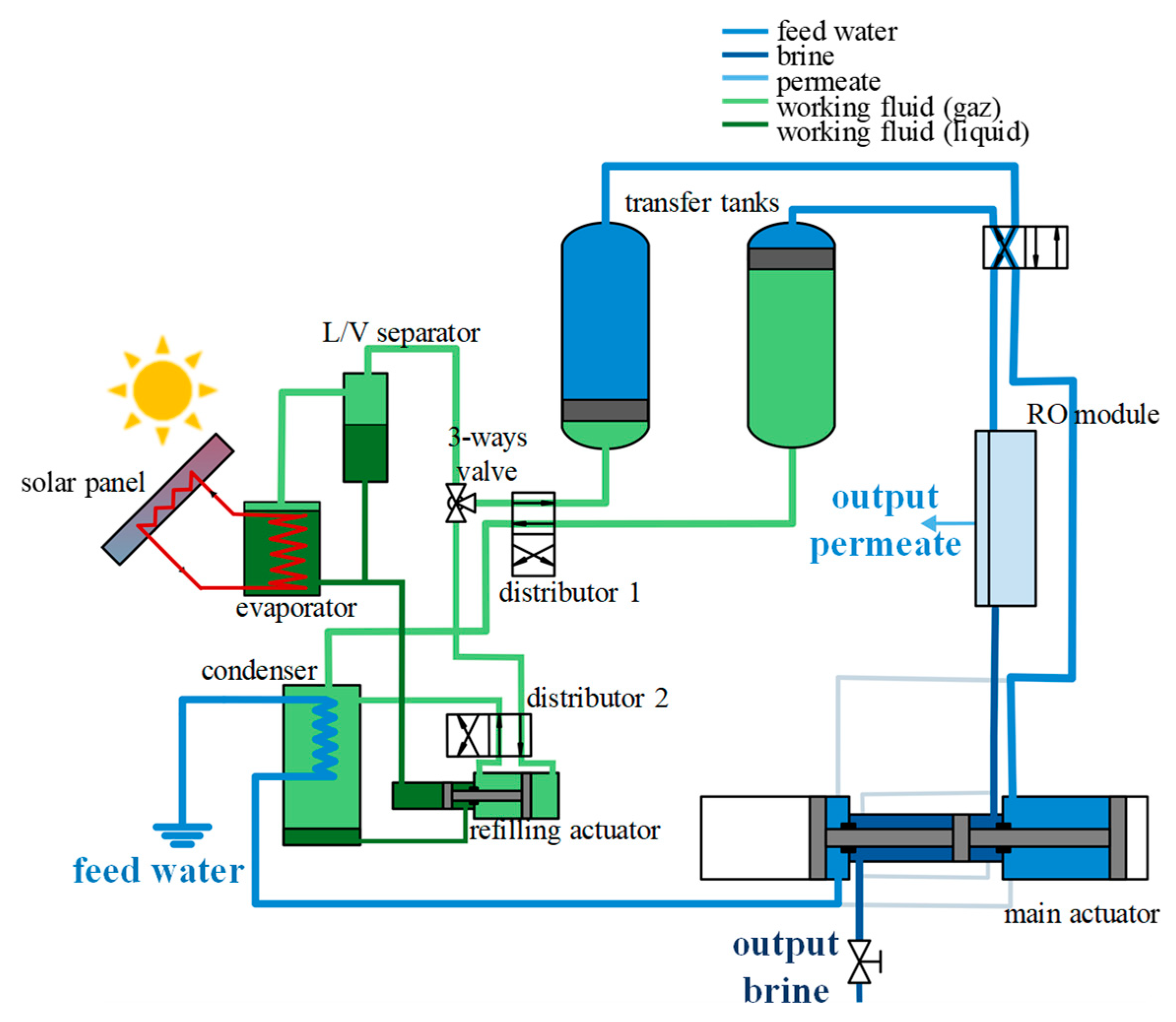
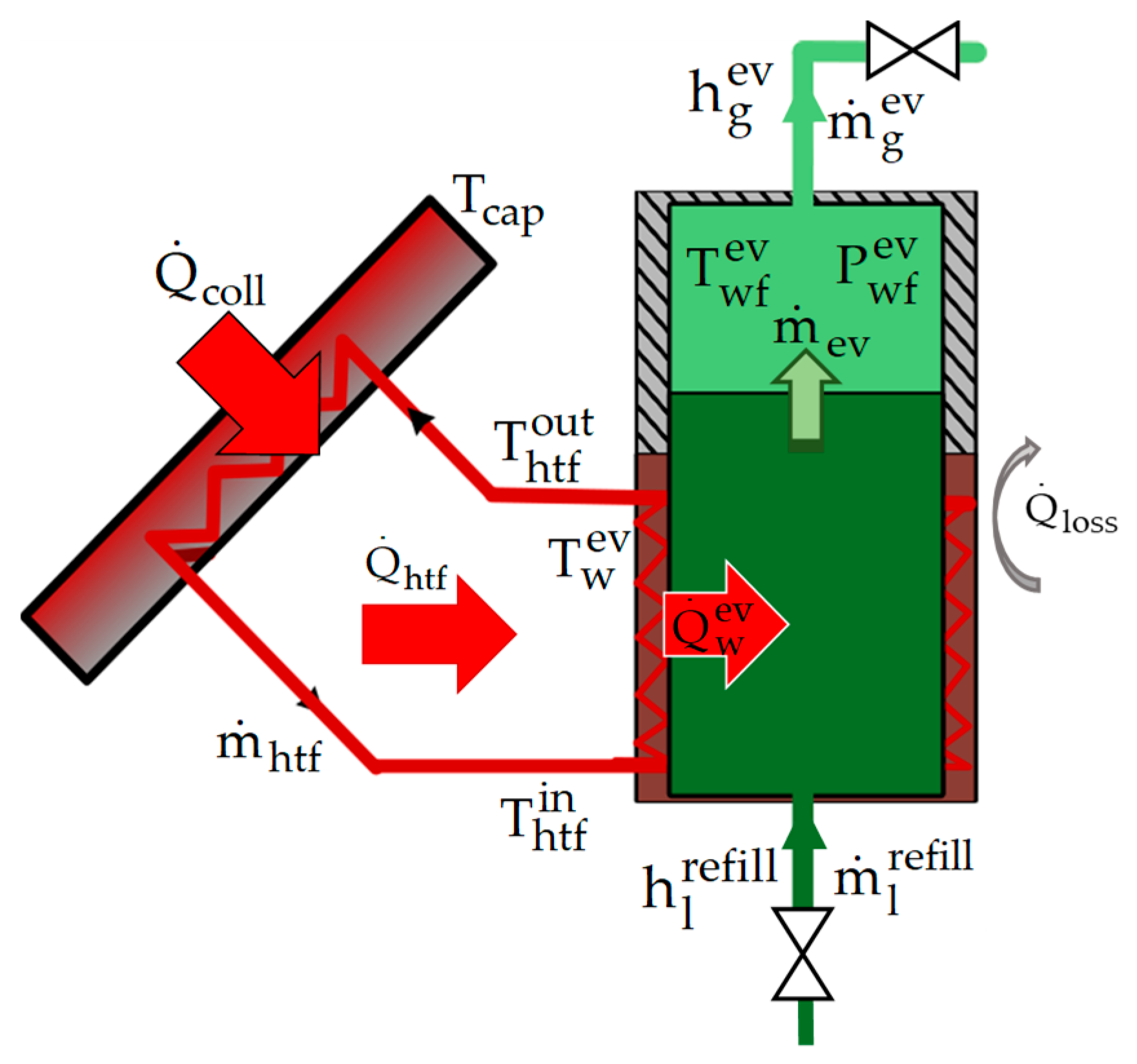
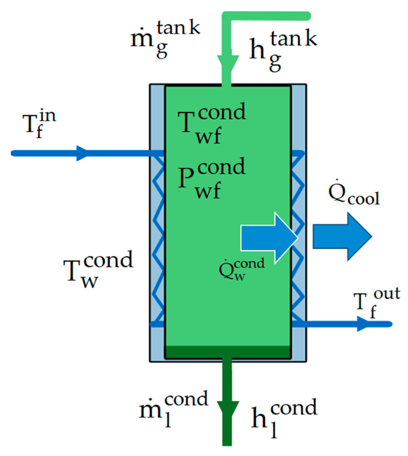
The engine cycle is composed of an evaporator heated by solar flat-plate collectors, and a condenser cooled by the saltwater to be desalinated. The high-pressure vapor of the working fluid that is generated by the evaporator flows into a first transfer tank filled with feed water and pressurizes it above its osmotic pressure. The condenser enables the condensation of the working fluid previously accumulated in a second low-pressure tank.

The pressurization of the water in the tank is realized thanks to an elastically deformable membrane which transfers the mechanical energy from the high-pressure working fluid to the feed water. The working fluid vapor is produced by the evaporator at a pressure ranging from 10 to 20 bars, thanks to the heat delivered at about 50 to 80 °C by the solar collectors. The suitable working fluid for these required operating conditions and for the inflammability criterion has been found to be the sulfur dioxide (SO₂).

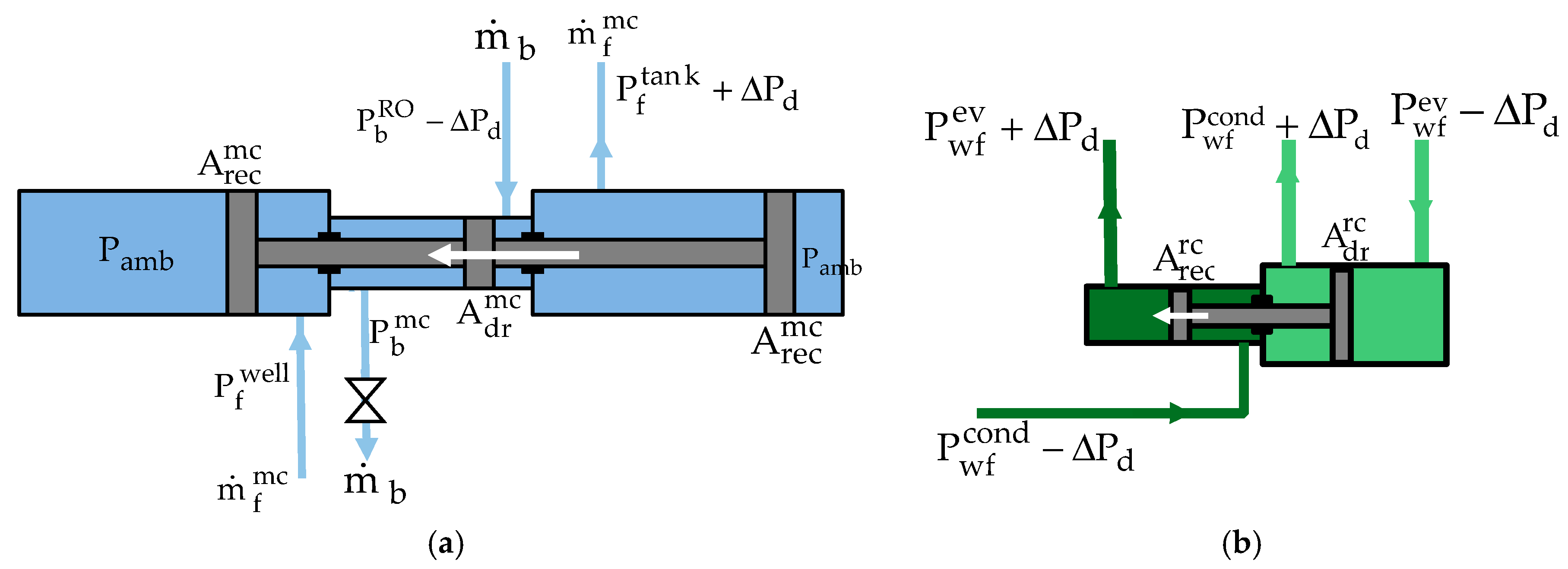
The hydraulic energy of the pressurized concentrated water (brine) flowing out of the RO module is recovered by a specific hydraulic cylinder (main actuator in Figure 1), which enables it to pump and fill the low-pressure reservoir with saltwater. A second hydraulic actuator (refiling actuator in Figure 1) is used to transfer the working fluid from the low-pressure condenser to the high-pressure evaporator. The main actuator is composed of three chambers in order to make it behave in a symmetric way in both directions of movement, that is to say, in order to ensure that the pumped and the pushed-back volumes of water inside the chambers are equal. The pressurization is done in the middle chamber that contains the driving piston, which transmits the mechanical energy and sets the piston in movement in the two lateral chambers in order to realize the pumping of the saltwater and the filling of the transfer tank. Thanks to this main hydraulic cylinder, the feed water to be desalinated is firstly pumped, then goes through the condenser, thus acting as a cold source for the thermodynamic cycle, and is temporarily accumulated in one of the lateral chambers of the hydraulic cylinder. Simultaneously, as the piston moves, the water to be desalinated, which was previously accumulated in the second lateral chamber of the hydraulic cylinder, is pushed out and pressurized in order to fill the low-pressure water tank connected to the condenser. At the same time, the feed water that is pressurized in the other tank by the high-pressure vapor of the engine cycle flows through the RO membrane. Clean water (permeate) is produced and the brine, which is still at high pressure, is used to drive the above-mentioned hydraulic cylinder.

Several distributors and valves allow for the role inversion of the reservoirs and the brine distribution in the process, as well as the control and cycling of the different operating steps of the process. The brine flow is controlled at the main cylinder outlet by a constant flow rate valve, which thus regulates the moving velocity of the cylinder piston.

The other independent actuator, which ensures the pressurization and the transfer of the liquid working fluid from the low-pressure condenser to the high-pressure evaporator tank, is set in motion by high-pressure vapor from the evaporator. The depressurized vapor in this cylinder flows into the condenser.

2.1. Description of the Cycle Phases

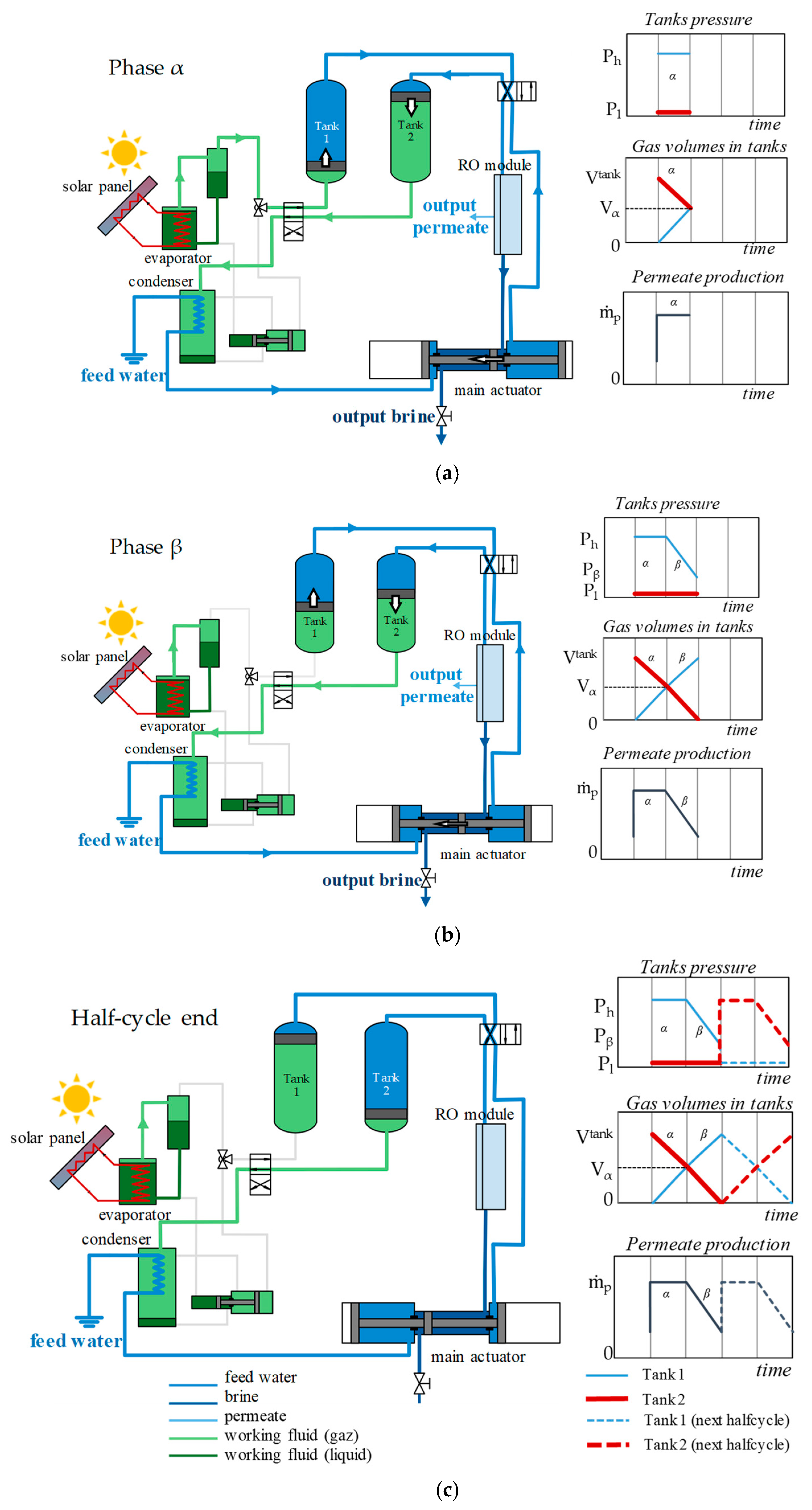
The operating cycle of the process consists of several steps described in Figure 2. An initialization phase enables pressurization at the high-pressure P_h of the transfer tank 1, which is already completely filled with saltwater, by connecting it to evaporator. Note that the high operating pressure has to be beyond the feed-water osmotic pressure to overcome transfer resistance throughout the RO membrane.

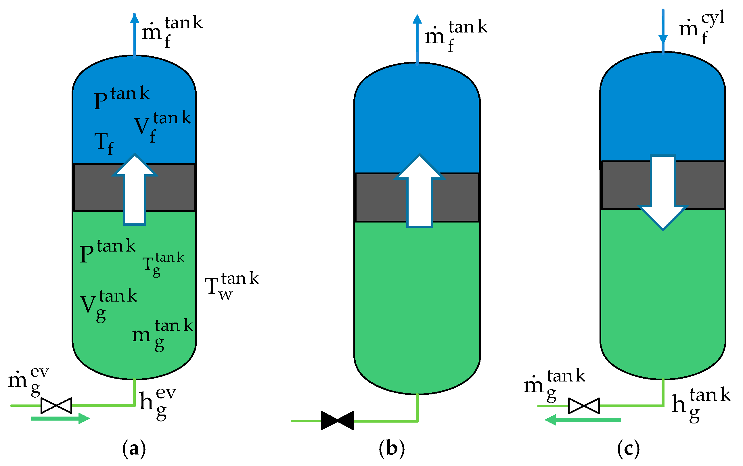
During the first step, or alpha phase (Figure 2a), the transfer tank 1 is linked to the evaporator, and the transfer tank 2 is connected with the condenser. The high-pressure feed water contained in the transfer tank 1 goes through the RO module and produces clean water under ideally constant pressure, P_h. The still-pressurized output brine is recovered and used by the main actuator to pump the saline water and fill the transfer tank 2 that is at the condenser pressure, P_l. The water filling the transfer tank 2 pushes out the vapors of the working fluid from that tank to the condenser, where it condenses at low pressure.

In the second step, or beta phase (Figure 2b), the transfer tank 1 is disconnected from the evaporator. Thus, the tank is no longer fed with high-pressure vapor. Nevertheless, the pressurized vapor contained in this tank continues to push out the saltwater to the RO membrane, generating an expansion of the gas (increasing the gas volume) and thus a decrease of the pressure until a minimum allowable pressure, P_β. That phase is also a desalination phase, but under a decreasing pressure, and thus enables a decreasing clean water production. At the end of this step, the transfer tank 2 is completely filled with feed water that will be later desalinated, and all of the working fluid previously contained in it has been expelled into the condenser. At this point, a half-cycle has been achieved (Figure 2c)—the first tank is then fully filled with vapor at the final pressure P_β of the beta phase, and the second one is full of saltwater at condenser pressure P_l. Distributors are then able to switch the tanks’ roles and run a new half-cycle.

Figure 2 also represents the volume and pressure evolutions of the working fluid vapor contained in each transfer tank. They respectively correspond to the feed tank volume V_α at the end of alpha phase at evaporator pressure P_h, the fully filled tank volume at the end of beta phase 2 at the end of phase pressure P_β, and the tank volume at condenser pressure P_l at the beginning of the next half-cycle after reversing the role of the feed tanks.

The design of the hydraulic cylinders (rod length, piston diameters, …) has been led in order to optimize the hydraulic energy recovery efficiency.

2.2. Refilling

Independently to the two presented phases, the refilling actuator permits refilling of the evaporator with liquid working fluid from the condenser. This cylinder is made with two chambers in which two pistons move with different diameters. The difference in the areas of the pistons allows for the pressure drop between the condenser and the evaporator to be overcome. The motor chamber is fed by the high-pressure vapor supplied by the evaporator, and sets the piston in motion (Figure 3). Then, the piston in the receiving chamber pressurizes, pushes out the liquid to the evaporator, and simultaneously sucks up the liquid from the condenser, and fills the chamber with liquid working fluid to be pressurized later. This refilling phase is activated when the liquid level of working fluid in the liquid/vapor separation tank of the flooded-type evaporator is low, and takes place during the beta phase when transfer tanks are disconnected with the evaporator.

In order to analyze the behavior and the performances of this process, dynamic modeling of the whole process has been developed and described in the following section.

3. Dynamic Process Modelling

The process has been modeled by considering a nodal approach. In this approach, all components of the system, except for the reverse osmosis membrane, are assumed to be at a uniform temperature, pressure, and concentration. The following main assumptions have been considered:

• Heat exchanged between and surrounding the process components are not taken into account, except for the evaporator that operates at a high temperature;
• Thermal equilibrium between the liquid and vapor phases in the evaporator and the condenser;
• Friction forces are negligible in the transfer tanks and pipes;
• Condensation effects are negligible in the actuators.

3.1. Solar Collector Coupled to the Evaporator

The evaporator is heated by a heat transfer fluid circulating between the solar collector and the evaporator, as shown in Figure 4.

In order to determine the heat flux transferred by the solar collector to the heat transfer fluid, the first law is applied to the solar collector:

$${\mathrm{m}}_{\mathrm{cap}}\mathrm{C}{\mathrm{p}}_{\mathrm{cap}}\frac{\mathrm{d}{\mathrm{T}}_{\mathrm{cap}}}{\mathrm{d}\mathrm{t}}={\dot{\mathrm{Q}}}_{\mathrm{coll}}-{\dot{\mathrm{Q}}}_{\mathrm{htf}}$$

(1)

where ${\dot{\mathrm{Q}}}_{\mathrm{coll}}$ is the solar flux collected and absorbed by the captor of area ${\mathrm{A}}_{\mathrm{cap}}$, and ${\dot{\mathrm{Q}}}_{\mathrm{htf}}$ is the heat flux transfer to the heat transfer fluid, which is exchanged with the evaporator wall. The collected solar heat flux is calculated by Equation (3) considering the collector efficiency ${\mathsf{\eta }}_{\mathrm{cap}}$, which is a function of the solar collector temperature T_cap, assumed to be equal to the mean temperature difference of the heat transfer fluid ${\mathrm{T}}_{\mathrm{cap}}=\left({\mathrm{T}}_{\mathrm{htf}}^{\mathrm{out}}+{\mathrm{T}}_{\mathrm{htf}}^{\mathrm{in}}\right)/2$, the ambient temperature T_amb, and the solar irradiation, I.

$${\dot{\mathrm{Q}}}_{\mathrm{htf}}={\dot{\mathrm{m}}}_{\mathrm{htf}}\mathrm{C}{\mathrm{p}}_{\mathrm{htf}}\left({\mathrm{T}}_{\mathrm{htf}}^{\mathrm{in}}-{\mathrm{T}}_{\mathrm{htf}}^{\mathrm{out}}\right)$$

(2)

$${\dot{\mathrm{Q}}}_{\mathrm{coll}}=\mathrm{I}{\mathrm{A}}_{\mathrm{cap}}{\mathsf{\eta }}_{\mathrm{cap}}=\mathrm{I}{\mathrm{A}}_{\mathrm{cap}}\left({\mathsf{\eta }}_{\mathrm{opt}}-\frac{{\mathrm{a}}_1\left({\mathrm{T}}_{\mathrm{cap}}-{\mathrm{T}}_{\mathrm{amb}}\right)}{\mathrm{I}}-\frac{{\mathrm{a}}_2{\left({\mathrm{T}}_{\mathrm{cap}}-{\mathrm{T}}_{\mathrm{amb}}\right)}^2}{\mathrm{I}}\right)$$

(3)

The temperature evolution of the evaporator wall ${\mathrm{T}}_{\mathrm{w}}^{\mathrm{ev}}$ and the heat rate exchange ${\dot{\mathrm{Q}}}_{\mathrm{w}}^{\mathrm{ev}}$ between the evaporator wall and the working fluid are determined by the following equations. The energy balance applied on the evaporator wall gives:

$${\mathrm{m}}_{\mathrm{w}}^{\mathrm{ev}}\mathrm{C}{\mathrm{p}}_{\mathrm{steel}}\frac{\mathrm{d}{\mathrm{T}}_{\mathrm{w}}^{\mathrm{ev}}}{\mathrm{d}\mathrm{t}}={\dot{\mathrm{Q}}}_{\mathrm{htf}}-{\dot{\mathrm{Q}}}_{\mathrm{w}}^{\mathrm{ev}}-{\dot{\mathrm{Q}}}_{\mathrm{loss}}$$

(4)

where ${\dot{\mathrm{Q}}}_{\mathrm{loss}}$ is the heat lost through convection:

$${\dot{\mathrm{Q}}}_{\mathrm{loss}}={\mathrm{k}}_{\mathrm{loss}}\left({\mathrm{T}}_{\mathrm{w}}^{\mathrm{ev}}-{\mathrm{T}}_{\mathrm{amb}}\right)$$

(5)

The heat flux transmitted to the evaporator wall is determined by considering heat exchanger effectiveness ${\mathsf{\epsilon }}_{\mathrm{ev}}$ between the evaporator, the evaporator wall, and the heat transfer fluid (see Equation (6)). The temperature change of the heat transfer fluid can then be expressed by Equation (7) as a function of the mean collector temperature, T_cap, and the evaporator wall temperature, ${\mathrm{T}}_{\mathrm{w}}^{\mathrm{ev}}$.

$${\mathsf{\epsilon }}^{\mathrm{ev}}=\frac{{\mathrm{T}}_{\mathrm{htf}}^{\mathrm{in}}-{\mathrm{T}}_{\mathrm{htf}}^{\mathrm{out}}}{{\mathrm{T}}_{\mathrm{htf}}^{\mathrm{in}}-{\mathrm{T}}_{\mathrm{w}}^{\mathrm{ev}}}$$

(6)

$${\mathrm{T}}_{\mathrm{htf}}^{\mathrm{in}}-{\mathrm{T}}_{\mathrm{htf}}^{\mathrm{out}}=\frac{2{\mathsf{\epsilon }}^{\mathrm{ev}}}{2-{\mathsf{\epsilon }}^{\mathrm{ev}}}\left({\mathrm{T}}_{\mathrm{cap}}-{\mathrm{T}}_{\mathrm{w}}^{\mathrm{ev}}\right)$$

(7)

The heat flux ${\dot{\mathrm{Q}}}_{\mathrm{htf}}$ that is transmitted to the evaporator wall from the solar collector can then be expressed as a function of the exchanger effectiveness and the mean collector temperature, (Equation (8)).

$${\dot{\mathrm{Q}}}_{\mathrm{htf}}={\dot{\mathrm{m}}}_{\mathrm{cap}}\mathrm{C}{\mathrm{p}}_{\mathrm{cap}}\frac{2{\mathsf{\epsilon }}^{\mathrm{ev}}}{2-{\mathsf{\epsilon }}^{\mathrm{ev}}}\left({\mathrm{T}}_{\mathrm{cap}}-{\mathrm{T}}_{\mathrm{w}}^{\mathrm{ev}}\right)$$

(8)

The heat that is transferred from the wall to the liquid working fluid in the evaporator is calculated by considering a convective heat exchange, as described in Equation (9), between the heated wall section and the liquid in touch:

$${\dot{\mathrm{Q}}}_{\mathrm{w}}^{\mathrm{ev}}={\mathrm{k}}_{\mathrm{l}}^{\mathrm{conv}}{\mathrm{S}}_{\mathrm{ev}}\left({\mathrm{T}}_{\mathrm{wf}}^{\mathrm{ev}}-{\mathrm{T}}_{\mathrm{w}}^{\mathrm{ev}}\right)$$

(9)

Then, the vapor and liquid mass variations are deduced from mass balances presented in Equations (10) and (11):

$$\frac{\mathrm{d}{\mathrm{m}}_{\mathrm{g}}^{\mathrm{ev}}}{\mathrm{d}\mathrm{t}}={\dot{\mathrm{m}}}_{\mathrm{ev}}-{\dot{\mathrm{m}}}_{\mathrm{g}}^{\mathrm{ev}}$$

(10)

and

$$\frac{\mathrm{d}{\mathrm{m}}_{\mathrm{l}}^{\mathrm{ev}}}{\mathrm{d}\mathrm{t}}={\dot{\mathrm{m}}}_{\mathrm{l}}^{\mathrm{refill}}-{\dot{\mathrm{m}}}_{\mathrm{ev}}$$

(11)

where ${\dot{\mathrm{m}}}_{\mathrm{ev}}$ is the evaporation rate of the working fluid, and ${\dot{\mathrm{m}}}_{\mathrm{l}}^{\mathrm{refill}}$ is the mass flow rate of the liquid coming from the condenser.

The vapor flow rate ${\dot{\mathrm{m}}}_{\mathrm{g}}^{\mathrm{ev}}$ that leaves the evaporator and flows to the transfer tank in order to pressurize the feed water is determined by the Equation (11) by considering the characteristics of the valve between the evaporator and the reservoir, that is, its flow coefficient K_v, and the pressure difference existing between them [25].

$${\mathrm{Q}}_{\mathrm{v}}=514.\mathrm{K}\mathrm{v}\sqrt{\frac{{\mathsf{\rho }}_{\mathrm{air}}}{{\mathsf{\rho }}_{\mathrm{g}}}\frac{\Delta {\mathrm{P}}_{\mathrm{v}}.{\mathrm{P}}_{\mathrm{g}}^{\mathrm{tank}}}{{\mathrm{T}}_{\mathrm{wf}}^{\mathrm{ev}}}}$$

(12)

This evaporation rate of the working fluid is determined from a chemical affinity law [26] that takes into account the thermodynamic unbalance between the vapor and the liquid phase, and is given by Equation (12) as a function of saturation pressure at the evaporator temperature and the actual evaporator pressure:

$${\dot{\mathrm{m}}}_{\mathrm{ev}}=\mathrm{K}\mathrm{c}\mathrm{i}{\mathrm{n}}_{\mathrm{ev}}\ln \left(\frac{{\mathrm{P}}_{\mathrm{sat}}\left({\mathrm{T}}_{\mathrm{wf}}^{\mathrm{ev}}\right)}{{\mathrm{P}}_{\mathrm{wf}}^{\mathrm{ev}}}\right)$$

(13)

where Kcin_ev is a chemical affinity coefficient that has to be adjusted.

The internal energy variation of the system composed of the liquid and the vapor in the evaporator can then be calculated by the first law of thermodynamics in Equation (14):

$$\frac{\mathrm{d}{\mathrm{U}}^{\mathrm{ev}}}{\mathrm{d}\mathrm{t}}={\dot{\mathrm{Q}}}_{\mathrm{w}}^{\mathrm{ev}}+{\dot{\mathrm{m}}}_{\mathrm{l}}^{\mathrm{refill}}{\mathrm{h}}_{\mathrm{l}}^{\mathrm{refill}}-{\dot{\mathrm{m}}}_{\mathrm{ev}}{\mathrm{h}}_{\mathrm{g}}^{\mathrm{ev}}\left({\mathrm{T}}_{\mathrm{wf}}^{\mathrm{ev}},{\mathsf{\rho }}_{\mathrm{g}}^{\mathrm{ev}}\right)$$

(14)

where the incoming liquid enthalpy is taken at the condenser pressure at a saturated liquid state. The internal energy of this system is the sum of vapor and liquid internal energies calculated in Equation (14) by the CoolProp equations of state as a function of the temperature and densities of each phase, and by assuming a thermal equilibrium between the two phases:

$${\mathrm{U}}^{\mathrm{ev}}={\mathrm{m}}_{\mathrm{l}}^{\mathrm{ev}}{\mathrm{u}}_{\mathrm{l}}^{\mathrm{ev}}\left({\mathrm{T}}_{\mathrm{wf}}^{\mathrm{ev}},{\mathsf{\rho }}_{\mathrm{l}}^{\mathrm{ev}}\right)+{\mathrm{m}}_{\mathrm{g}}^{\mathrm{ev}}{\mathrm{u}}_{\mathrm{g}}^{\mathrm{ev}}\left({\mathrm{T}}_{\mathrm{wf}}^{\mathrm{ev}},{\mathsf{\rho }}_{\mathrm{g}}^{\mathrm{ev}}\right)$$

(15)

The working fluid temperature can then be calculated by numerical resolution from Equation (15).

The evaporator pressure can then be obtained from the CoolProp equation of state (Equation (16)).

$${\mathrm{P}}_{\mathrm{wf}}^{\mathrm{ev}}=\mathrm{f}\left({\mathrm{T}}_{\mathrm{wf}}^{\mathrm{ev}},{\mathsf{\rho }}_{\mathrm{g}}^{\mathrm{ev}}\right)$$

(16)

3.2. Condenser

The condenser modeling is quite similar to the evaporator one. It is assumed here that there is a constant liquid volume in the condenser, as the working fluid condensate is instantaneously evacuated in the reservoir and thus the liquid level is kept constant, as shown in Figure 5. A minimum liquid quantity is nonetheless required for the thermodynamic equilibrium hypothesis to be acceptable.

The heat of condensation is evacuated by the feed water, whose inlet temperature is known. The heat flux is also expressed, as Equation (17) shows, by considering exchanger effectiveness.

$${\dot{\mathrm{Q}}}_{\mathrm{cool}}={\dot{\mathrm{m}}}_{\mathrm{f}}.\mathrm{C}{\mathrm{p}}_{\mathrm{f}}\left({\mathrm{T}}_{\mathrm{f}}^{\mathrm{out}}-{\mathrm{T}}_{\mathrm{f}}^{\mathrm{in}}\right)$$

(17)

The condenser wall temperature and the internal energy of the working fluid, pressure, and temperature are calculated by the set of Equations (19)–(24). These equations are similar to the evaporator ones, that is, from mass and energy balances. By knowing the initial state of the condenser, the evolution of the condenser is then determined. The first law of thermodynamics (energy conservation) can be applied to the condenser wall as:

$${\mathrm{m}}_{\mathrm{w}}^{\mathrm{cond}}\mathrm{C}{\mathrm{p}}_{\mathrm{steel}}\frac{\mathrm{d}{\mathrm{T}}_{\mathrm{w}}^{\mathrm{cond}}}{\mathrm{d}\mathrm{t}}={\dot{\mathrm{Q}}}_{\mathrm{w}}^{\mathrm{cond}}-{\dot{\mathrm{Q}}}_{\mathrm{cool}}$$

(18)

where the heat transfer between the wall condenser and the working fluid is given by the Newton law:

$${\dot{\mathrm{Q}}}_{\mathrm{w}}^{\mathrm{cond}}={\mathrm{k}}_{\mathrm{cond}}^{\mathrm{conv}}{\mathrm{S}}_{\mathrm{cond}}\left({\mathrm{T}}_{\mathrm{wf}}^{\mathrm{cond}}-{\mathrm{T}}_{\mathrm{w}}^{\mathrm{cond}}\right)$$

(19)

The mass balance applied to the gas gives the following, considering the fixed condenser volume control:

$$\frac{\mathrm{d}{\mathrm{m}}_{\mathrm{g}}^{\mathrm{cond}}}{\mathrm{d}\mathrm{t}}={\dot{\mathrm{m}}}_{\mathrm{g}}^{\tan \mathrm{k}}-{\dot{\mathrm{m}}}_{\mathrm{cond}}$$

(20)

The internal energy variation of the working fluid is also given by the first principle:

$$\frac{\mathrm{d}{\mathrm{U}}^{\mathrm{cond}}}{\mathrm{d}\mathrm{t}}=-{\dot{\mathrm{Q}}}_{\mathrm{w}}^{\mathrm{cond}}-{\dot{\mathrm{m}}}_{\mathrm{l}}^{\mathrm{cond}}{\mathrm{h}}_{\mathrm{l}}^{\mathrm{cond}}+{\dot{\mathrm{m}}}_{\mathrm{g}}^{\mathrm{cond}}{\mathrm{h}}_{\mathrm{g}}^{\mathrm{cond}}$$

(21)

where the internal energy is expressed as:

$${\mathrm{U}}^{\mathrm{cond}}={\mathrm{m}}_{\mathrm{l}}^{\mathrm{cond}}{\mathrm{u}}_{\mathrm{l}}^{\mathrm{cond}}\left({\mathrm{T}}_{\mathrm{wf}}^{\mathrm{cond}},{\mathsf{\rho }}_{\mathrm{l}}^{\mathrm{cond}}\right)+{\mathrm{m}}_{\mathrm{g}}^{\mathrm{cond}}{\mathrm{u}}_{\mathrm{g}}^{\mathrm{cond}}\left({\mathrm{T}}_{\mathrm{wf}}^{\mathrm{cond}},{\mathsf{\rho }}_{\mathrm{g}}^{\mathrm{cond}}\right)$$

(22)

The working fluid pressure can be obtained by a CoolProp equation of state as a function of its temperature and its liquid or gas density:

$${\mathrm{P}}_{\mathrm{wf}}^{\mathrm{cond}}=\mathrm{f}\left({\mathrm{T}}_{\mathrm{wf}}^{\mathrm{cond}},{\mathsf{\rho }}_{\mathrm{g}}^{\mathrm{cond}}\right)$$

(23)

Finally, the condensation flow can be given by a chemical affinity law:

$${\dot{\mathrm{m}}}_{\mathrm{cond}}={\dot{\mathrm{m}}}_{\mathrm{l}}^{\mathrm{cond}}=\mathrm{K}\mathrm{c}\mathrm{i}{\mathrm{n}}_{\mathrm{cond}}\ln \left(\frac{{\mathrm{P}}_{\mathrm{wf}}^{\mathrm{cond}}}{{\mathrm{P}}_{\mathrm{sat}}\left({\mathrm{T}}_{\mathrm{wf}}^{\mathrm{cond}}\right)}\right)$$

(24)

3.3. Transfer Tanks

In the transfer tanks, the feed water and the working fluid are physically separated by a deformable or movable frontier. Thus, this physical separation is not necessarily a mobile piston, like that represented in the schema of Figure 6. It can be an elastically deformable membrane or a bladder with a low deformation resistance, so the hypothesis of a pressure equilibrium between the water and the vapor working fluid is considered.

The evolution of the saline water and gaseous working fluid volumes that are present in the transfer tanks are calculated from the mass flow rate of feed water that enters or leaves the transfer tank:

$$\frac{\mathrm{d}{\mathrm{V}}_{\mathrm{g}}^{\mathrm{tank}}}{\mathrm{d}\mathrm{t}}=-\frac{\mathrm{d}{\mathrm{V}}_{\mathrm{f}}^{\mathrm{tank}}}{\mathrm{d}\mathrm{t}}=\frac{{\dot{\mathrm{m}}}_{\mathrm{f}}^{\mathrm{tank}}}{{\mathsf{\rho }}_{\mathrm{f}}}$$

(25)

During the high-pressure phase, the working fluid may partially condense on the walls, leading to an additional pressure decrease. This condensation is due to the cooling of the tank wall during the previous half-cycle by the cold feed saltwater, making the wall cooler than the saturation temperature of the input high-pressure gas. This phenomenon is taken into account throughout Equation (30) in a similar way as to the condenser modeling, and enables assessment of the condensation rate of the vapor on the tank walls. This transfer tank modeling leads to another set of equations also based on mass and energy balances (Equations (26)–(28)), as well as CoolProp state equations (Equation (29)). The mass balance applied on the gas volume gives:

$$\frac{\mathrm{d}{\mathrm{m}}_{\mathrm{g}}^{\tan \mathrm{k}}}{\mathrm{d}\mathrm{t}}={\dot{\mathrm{m}}}_{\mathrm{g}}^{\tan \mathrm{k}}-{\dot{\mathrm{m}}}_{\mathrm{cond}}$$

(26)

where the mass of gaseous working fluid can be obtained by its density from a CoolProp equation of state:

$${\mathrm{m}}_{\mathrm{g}}^{\tan \mathrm{k}}={\mathrm{V}}_{\mathrm{g}}^{\tan \mathrm{k}}{\mathsf{\rho }}_{\mathrm{g}}^{\tan \mathrm{k}}\left({\mathrm{u}}_{\mathrm{g}}^{\tan \mathrm{k}},{\mathrm{P}}_{\mathrm{g}}^{\tan \mathrm{k}}\right)$$

(27)

The gas internal energy balance is given by the first law of thermodynamics:

$$\frac{\mathrm{d}\left({\mathrm{m}}_{\mathrm{g}}^{\tan \mathrm{k}}{\mathrm{u}}_{\mathrm{g}}^{\tan \mathrm{k}}\right)}{\mathrm{d}\mathrm{t}}={\dot{\mathrm{m}}}_{\mathrm{g}}^{\mathrm{ev}}{\mathrm{h}}_{\mathrm{g}}^{\mathrm{ev}}+{\dot{\mathrm{m}}}_{\mathrm{cond}}^{\tan \mathrm{k}}\Delta {\mathrm{h}}_{\mathrm{cond}}\left({\mathrm{T}}_{\mathrm{sat}}\left({\mathrm{P}}_{\mathrm{g}}^{\tan \mathrm{k}}\right)\right)-{\mathrm{P}}_{\mathrm{g}}^{\tan \mathrm{k}}\frac{\mathrm{d}{\mathrm{V}}_{\mathrm{g}}^{\tan \mathrm{k}}}{\mathrm{d}\mathrm{t}}$$

(28)

and the gas temperature can also be calculated by the equation of state of the working fluid:

$${\mathrm{T}}_{\mathrm{g}}^{\tan \mathrm{k}}=\mathrm{f}\left({\mathrm{u}}_{\mathrm{g}}^{\tan \mathrm{k}},{\mathrm{P}}_{\mathrm{g}}^{\tan \mathrm{k}}\right)$$

(29)

The condensation rate of the working fluid at the wall of the tank is also calculated by considering a chemical affinity law:

$${\dot{\mathrm{m}}}_{\mathrm{cond}}^{\mathrm{tank}}=\mathrm{K}\mathrm{c}\mathrm{i}{\mathrm{n}}_{\mathrm{cond}}\ln \left(\frac{{\mathrm{P}}_{\mathrm{g}}^{\mathrm{tank}}}{{\mathrm{P}}_{\mathrm{sat}}\left({\mathrm{T}}_{\mathrm{w}}^{\mathrm{tank}}\right)}\right)$$

(30)

The wall temperature is calculated from the energy balance expressed in Equation (31), as the energy exchange between the wall and the gas is mainly enthalpy of condensation.

$${\mathrm{m}}_{\mathrm{w}}^{\mathrm{tank}}\mathrm{C}{\mathrm{p}}_{\mathrm{steel}}\frac{\mathrm{d}{\mathrm{T}}_{\mathrm{w}}^{\mathrm{tank}}}{\mathrm{d}\mathrm{t}}={\dot{\mathrm{m}}}_{\mathrm{cond}}\Delta {\mathrm{h}}_{\mathrm{cond}}-{\dot{\mathrm{Q}}}_{\mathrm{loss}}$$

(31)

3.4. Hydraulic Cylinders

Cylinders are considered to be adiabatic. The pressure Pb of the output brine and the mass flow rate of the feed saltwater are calculated as described in Figure 7.

Cylinder modeling was developed by considering the strength balances applied to the main rod and pistons of given diameters. For the main cylinder, the forces equilibrium has been expressed as follows by considering a cylinder mechanical efficiency, k_f:

$${\mathrm{A}}_{\mathrm{dr}}^{\mathrm{mc}}\left({\mathrm{P}}_{\mathrm{b}}^{\mathrm{RO}}-\Delta {\mathrm{P}}_{\mathrm{d}}-{\mathrm{P}}_{\mathrm{b}}^{\mathrm{mc}}\right){\mathrm{k}}_{\mathrm{f}}={\mathrm{A}}_{\mathrm{rec}}^{\mathrm{mc}}\left({\mathrm{P}}_{\mathrm{f}}^{\tan \mathrm{k}}+\Delta {\mathrm{P}}_{\mathrm{d}}-{\mathrm{P}}_{\mathrm{f}}^{\mathrm{well}}\right)$$

(32)

ΔP_d corresponds to the pressure drop in the distributors. The output brine pressure can then be determined as follows by taking into account the efficiency of the cylinder:

$${\mathrm{P}}_{\mathrm{b}}^{\mathrm{mc}}=\left({\mathrm{P}}_{\mathrm{b}}^{\mathrm{RO}}-\Delta {\mathrm{P}}_{\mathrm{d}}\right)-\left({\mathrm{P}}_{\mathrm{f}}^{\tan \mathrm{k}}+\Delta {\mathrm{P}}_{\mathrm{d}}-{\mathrm{P}}_{\mathrm{f}}^{\mathrm{well}}\right)\frac{{\mathrm{A}}_{\mathrm{rec}}^{\mathrm{mc}}}{{\mathrm{A}}_{\mathrm{dr}}^{\mathrm{mc}}.{\mathrm{k}}_{\mathrm{f}}}$$

(33)

The mass flow rate of the pumped feed water from the well and of the tank feed water filling are given by the piston speeds’ equality, as expressed in Equation (34):

$$\frac{{\dot{\mathrm{V}}}_{\mathrm{b}}}{{\mathrm{A}}_{\mathrm{dr}}^{\mathrm{mc}}}=\frac{{\dot{\mathrm{V}}}_{\mathrm{f}}^{\mathrm{mc}}}{{\mathrm{A}}_{\mathrm{rec}}^{\mathrm{mc}}}$$

(34)

which gives:

$${\dot{\mathrm{m}}}_{\mathrm{f}}^{\mathrm{mc}}=\frac{{\mathrm{A}}_{\mathrm{rec}}^{\mathrm{mc}}}{{\mathrm{A}}_{\mathrm{dr}}^{\mathrm{mc}}}{\dot{\mathrm{m}}}_{\mathrm{b}}\frac{{\mathsf{\rho }}_{\mathrm{f}}}{{\mathsf{\rho }}_{\mathrm{b}}}$$

(35)

where ṁ_b is the mass flow rate of the outlet brine that is controlled and regulated to a fixed value depending on the evaporator pressure. A similar force balance is applied to the second cylinder which has only two chambers, and leads to Equation (36):

$${\mathrm{A}}_{\mathrm{dr}}^{\mathrm{rc}}\left({\mathrm{P}}_{\mathrm{wf}}^{\mathrm{ev}}-\Delta {\mathrm{P}}_{\mathrm{d}}-\left({\mathrm{P}}_{\mathrm{wf}}^{\mathrm{cond}}+\Delta {\mathrm{P}}_{\mathrm{d}}\right)\right){\mathrm{k}}_{\mathrm{f}}={\mathrm{A}}_{\mathrm{rec}}^{\mathrm{rc}}\left({\mathrm{P}}_{\mathrm{wf}}^{\mathrm{ev}}+\Delta {\mathrm{P}}_{\mathrm{d}}-\left({\mathrm{P}}_{\mathrm{wf}}^{\mathrm{cond}}-\Delta {\mathrm{P}}_{\mathrm{d}}\right)\right)$$

(36)

It can be seen in Equation (35) that the motor piston has to be bigger than the receiver piston in order to overcome the pressure losses due to the check valve placed upstream and downstream of the cylinder and the friction dissipation occurring in the cylinder.

3.5. Reverse Osmosis Membrane

Particular attention was drawn to the reverse osmosis membrane implemented in the spiral wound module. A nodal modeling that considers uniform value in this element is not suitable and cannot correctly represent the dynamic behavior of the permeation through the RO membrane. For this reason, a 1D modeling has been carried out and validated on a test bench in order to better understand the dynamic cycle impacts on the membrane performances.

In this modeling approach, variable input parameters, such as mass flow rate, pressure, and salt concentration were applied at the feed side. The outputs were mass flow rate, pressure, and salt concentration of the output brine and permeate, as detailed in Figure 8.

The reverse osmosis dynamic model was established considering the following assumptions:

• The salt water and permeate are considered to be an incompressible fluid with a constant density;
• No membrane compaction is assumed;
• The pressure is homogeneous in the permeate channel;
• The permeate concentration is considered homogenous according to the radial direction;
• The RO process is considered isothermal.

The mass conservation equation applied to the module can be expressed as follows by considering that the saltwater is neither compressible nor expansible in the membrane channel. This balance thus results in:

$${\dot{\mathrm{m}}}_{\mathrm{f}}^{\mathrm{RO}}\left(0,\mathrm{t}\right)={\dot{\mathrm{m}}}_{\mathrm{f}}^{\mathrm{RO}}\left(\mathrm{L},\mathrm{t}\right)+{\dot{\mathrm{m}}}_{\mathrm{p}}^{\mathrm{RO}}\left(\mathrm{L},\mathrm{t}\right)$$

(37)

Permeate flow can be expressed as a function of the water flux, Jw, and the salt flux, Js:

$${\dot{\mathrm{m}}}_{\mathrm{p}}^{\mathrm{RO}}\left(\mathrm{L},\mathrm{t}\right)=\mathrm{W}\left({\mathsf{\rho }}_{\mathrm{w}}{\displaystyle {\int }_0^{\mathrm{L}}{\mathrm{J}}_{\mathrm{w}}\left(\mathrm{x},\mathrm{t}\right)}\mathrm{d}\mathrm{x}+{\displaystyle {\int }_0^{\mathrm{L}}{\mathsf{\rho }}_{\mathrm{s}}\left(\mathrm{x},\mathrm{t}\right){\mathrm{J}}_{\mathrm{s}}\left(\mathrm{x},\mathrm{t}\right)\mathrm{d}\mathrm{x}}\right)$$

(38)

Similarly, the species conservation, that is, the variation of the mass of dissolved salt between the membrane input and outputs can also be expressed, respectively, at the feed side and the permeate side, as:

$$\frac{\mathrm{d}}{\mathrm{d}\mathrm{t}}\left[{\displaystyle {\int }_0^{\mathrm{L}}{\mathrm{M}}_{\mathrm{f}}^{\mathrm{RO}}\left(\mathrm{x}\right){\mathrm{C}}_{\mathrm{f}}\left(\mathrm{x},\mathrm{t}\right)}\mathrm{d}\mathrm{x}\right]={\dot{\mathrm{m}}}_{\mathrm{f}}^{\mathrm{RO}}\left(0,\mathrm{t}\right){\mathrm{C}}_{\mathrm{f}}\left(0,\mathrm{t}\right)-\left({\dot{\mathrm{m}}}_{\mathrm{f}}^{\mathrm{RO}}\left(\mathrm{L},\mathrm{t}\right){\mathrm{C}}_{\mathrm{f}}\left(\mathrm{L},\mathrm{t}\right)+\mathrm{W}{\displaystyle {\int }_0^{\mathrm{L}}{\mathsf{\rho }}_{\mathrm{s}}\left(\mathrm{x},\mathrm{t}\right){\mathrm{J}}_{\mathrm{s}}\left(\mathrm{x},\mathrm{t}\right)}\mathrm{d}\mathrm{x}\right)$$

(39)

$$\frac{\mathrm{d}}{\mathrm{d}\mathrm{t}}\left[{\displaystyle {\int }_0^{\mathrm{L}}{\mathrm{M}}_{\mathrm{p}}^{\mathrm{RO}}\left(\mathrm{x}\right){\mathrm{C}}_{\mathrm{p}}\left(\mathrm{x},\mathrm{t}\right)}\mathrm{d}\mathrm{x}\right]=\mathrm{W}{\displaystyle {\int }_0^{\mathrm{L}}{\mathsf{\rho }}_{\mathrm{s}}\left(\mathrm{x},\mathrm{t}\right){\mathrm{J}}_{\mathrm{s}}\left(\mathrm{x},\mathrm{t}\right)}\mathrm{d}\mathrm{x}-{\dot{\mathrm{m}}}_{\mathrm{p}}^{\mathrm{RO}}\left(\mathrm{L},\mathrm{t}\right){\mathrm{C}}_{\mathrm{p}}\left(\mathrm{L},\mathrm{t}\right)$$

(40)

These equations allow for determination at each time, the mass flows and concentrations of feed saltwater, brine and permeate, provided the water and salt flux across the membrane, Jw and Js, are known. These fluxes are determined with the following mass transfer laws. Lonsdale et al. [27] developed a model to characterize the solvent (Equation (41)) and solute (Equation (42)) transfers across a semi-permeable membrane. The water transfer law is a Darcy-based law, as it is driven by the difference of applied pressure and osmotic pressure across the membrane. The solute transfer obeys a Fick transfer law and is driven by the difference of salt concentration existing at the membrane walls of the feed channel and permeate channel.

$${\mathrm{J}}_{\mathrm{w}}\left(\mathrm{x},\mathrm{t}\right)={\mathrm{L}}_{\mathrm{w}}\left(\Delta {\mathrm{P}}_{\mathrm{m}}\left(\mathrm{x},\mathrm{t}\right)-\Delta \mathsf{\pi }\left(\mathrm{x},\mathrm{t}\right)\right)$$

(41)

$${\mathrm{J}}_{\mathrm{s}}\left(\mathrm{x},\mathrm{t}\right)={\mathrm{L}}_{\mathrm{s}}\left({\mathrm{C}}_{\mathrm{m}}\left(\mathrm{x},\mathrm{t}\right)-{\mathrm{C}}_{\mathrm{p}}\left(\mathrm{x},\mathrm{t}\right)\right)$$

(42)

The water flux is only possible when the applied pressure difference is beyond the osmotic pressure difference, which is proportional to the salt concentration and water temperature (Equation (43)):

$$\mathsf{\pi }={\mathrm{m}}_{\mathrm{i}}\mathrm{CRT}$$

(43)

where m_i corresponds to the molality number, depending on the dissociation coefficient $\mathsf{\varphi }$. Then, the osmotic pressure difference can be expressed as follows:

$$\Delta \mathsf{\pi }\left(\mathrm{x},\mathrm{t}\right)=2\mathsf{\varphi }\frac{{\mathsf{\rho }}_{\mathrm{NaCl}}}{{\widehat{\mathrm{M}}}_{\mathrm{NaCl}}}\mathrm{R}{\mathrm{T}}_{\mathrm{f}}\left({\mathrm{C}}_{\mathrm{m}}\left(\mathrm{x},\mathrm{t}\right)-{\mathrm{C}}_{\mathrm{p}}\left(\mathrm{x},\mathrm{t}\right)\right)$$

(44)

The water flux across the membrane is impacted by the salt concentration C_m at the membrane wall, which is different from the bulk concentration due to the appearance of the diffusive layer at the membrane wall. This layer, also called the polarization layer, induces a salt concentration increase at the membrane wall. A low Sherwood number, which can be observed for a low feed flowrate case, will induce a thick diffusive layer, as described in Figure 9.

The polarization layer modelling is detailed in Appendix A. Given the lack of studies on RO for this kind of dynamic, an experimental study was then carried out to calibrate this modelling and compare the numerical results.

4. Experimental Study

Experiments were conducted to assess the RO membrane behavior facing dynamic applied pressure and flow constraints. The aim was to compare the experimental data with numerical simulation results in order to build a dynamic predictive model of RO membrane desalination. For this experimental study, a brackish water desalination test bench was set up to operate an RO module under steady or dynamic conditions. Experiments were performed by controlling the evolution of the feed pressure at the inlet of the module and brine flow at the outlet of the module.

4.1. Experimental Setup

The test bench is presented in Figure 10 and consists of two tanks: one pressurized by a controlled high-pressure nitrogen line, while the second tank was emptying at atmospheric pressure. Feed water was directly pressurized in the feed tank with the nitrogen gas, and the valves allowed for the pressurized feed water to circulate thoughout the membrane. The produced permeate was collected and continuously weighted, while the membrane output brine filled the second tank at a nearly atmospheric pressure. The concentrated brine flow rate was controlled and regulated at the outlet of the RO module. The water loop was designed to measure the water flows, pressures, and salinities at the inlet and outlet of the RO module. A pressure regulator maintained the permeate pressure to a value near to the atmospheric pressure to ensure maximal trans-membrane pressure.

The test bench was instrumented with the sensors listed in

Table 1. Sensors description.

Quantity	Sensor	Reference	Range	Accuracy
2	Pressure	KROHNE Optibar 1010C	0–25 bars	±0.25% of max. scale
1	Pressure	KELLER PAA-23S	0–5 bars	±0.2% of max. scale
2	Conductimeter	JUMO CTI-750	0–20 mS·cm−1	±0.5% of max. scale
1	Conductimeter	KROHNE Cond3200	1–1000 µS·cm−1	±3% of measure
1	Flowmeter	KOBOLD DRH-1515	0.3–2.8 L·min−1	±2.5% of max. scale
1	Weighing scale	SCAIME AL5	0–5 kg	±0.017% of max. scale
2	Level gauge	ENDRESS HAUSER	0.1–500 mm	±0.1% of measure

with their measurement range and accuracy. Level gauges installed in the tanks also enabled determination of the water that flowed in or out of the tanks. Permeate production was measured continuously with a connected weighing scale. Measurement of water temperature was realized in the tanks. Three inductive conductimeters enabled determination of the salt concentrations of feed saltwater, brine, and clean water, thanks to the relation given by Aminot et al. [28].

The RO module is a spiral wound membrane designed by DOW Company (TW30-2514) for low salt concentrations, up to 10 g·L⁻¹, and was adapted for brackish water desalination. The membrane was chosen for its compatibility with low flow rates and its wide feed salinity range use. Its geometrical and transfer properties are given in

Table 2. Geometrical and transfer characteristics of the tested reverse osmosis (RO) module.

RO Module Characteristics	Value (TW30-2514)
Feed channel thickness thf	0.7 mm
Permeate channel thickness thp	0.7 mm
Area Am	0.59 m²
Length L	0.295 m
Water Permeability Lw	1.7.10−11 m3·m−2·Pa−1·s−1
Salt permeability Ls	3.5.10−11 m·s−1

. Note that the water and salt permeabilities have been experimentally determined on the presented test bench under stationary regime tests, that is, with constant pressure applied. These calculated permeabilities match with nominal performances given by the manufacturer’s data sheet.

4.2. Model Comparison

A parametrical identification was conducted to calibrate the previously introduced dynamic modeling to match it with the experimental results. The chosen adjusting parameter is the salt diffusion coefficient, which is calculated from a specific correlation (see Appendix A).

Permeate flow and brine concentration resulting from the calibrated dynamic model were then compared to the experimental data for similar operating conditions, that is, applied feed pressure shown in Figure 11, feed concentration, and retentate flow. Results are compared in Figure 12 throughout a dimensionless brine concentration, C_dim expressed by the ratio of the brine concentration to the inlet feed concentration, and the recovery rate, Y, expressed as the ratio of the permeate flow to the inlet feed saltwater flow, as defined in Equations (45) and (46).

$${\mathrm{C}}_{\dim }=\frac{{\mathrm{C}}_{\mathrm{b}}}{{\mathrm{C}}_{\mathrm{f}}}$$

(45)

$$\mathrm{Y}=\frac{{\dot{\mathrm{m}}}_{\mathrm{p}}^{\mathrm{RO}}}{{\dot{\mathrm{m}}}_{\mathrm{f}}^{\mathrm{RO}}}$$

(46)

The studied evolution is the decrease of the applied pressure, which results from the expansion of the pressurized nitrogen gas in the closed feed tank, described in Figure 11. The tests were performed for three pressure profiles at different starting pressures of the feed tank (bars 7, 10, and 12) represented in Figure 12. The feed saltwater concentration was maintained at around 4 g·L⁻¹ and the retentate flow was regulated and maintained to a constant value of around 0.15 L/min.

Figure 12 shows that the permeate flow and brine concentration decreases when the feed pressure decreases. This evolution is normal, as the permeate flow is proportional to the trans-membrane pressure that is thus decreasing. Relative errors from the dimensionless retentate concentration comparison all are under 5%, and under 10% for the recovery rate. There is an exception for the recovery rate at 7 bars, where the numerical data has a relative error of about 35% due to experimental points dispersion in the static part, and this error drops to 20% in the dynamic part. From this comparison, the numerical model seems to be representative of the dynamic behavior of the RO module, giving the scale of the study. These tests allowed us to consider that the RO dynamic modeling presented here gave sufficiently accurate adequacy between simulated and experimental results, and thus can be considered as validated for the whole modeling process.

5. Process Simulations and Results

Once the dynamic modeling was fully established, it was implemented to assess the whole process behavior during a complete day. Simulation parameters were determined from a previous sizing, and simulations were made under static working conditions.

Before the RO model integration in the complete process modeling, an additional study was conducted on local variations along the membrane channels. This local study aimed to evaluate the impact on the membrane’s local performances of a pressure steep variation, similar to the one involved in the process.

5.1. Axial Concentration Evolution Study

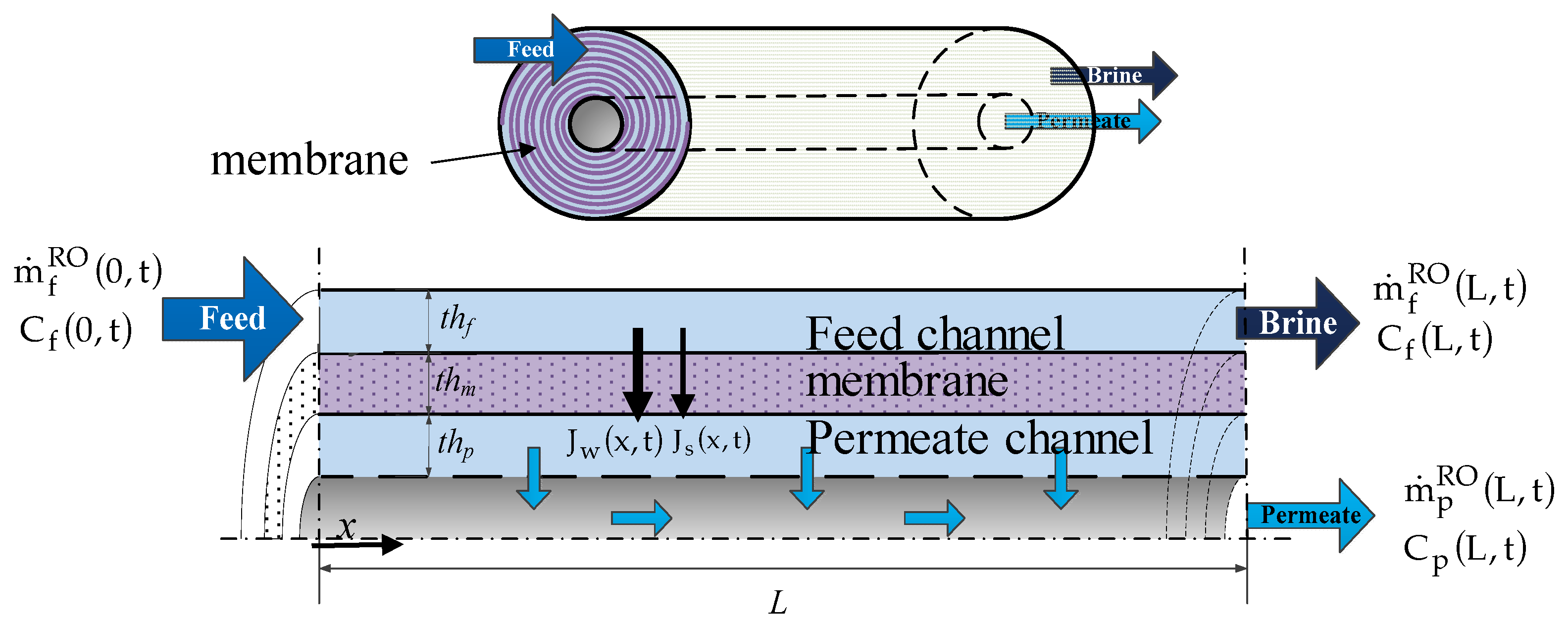
The dynamic model also enables characterization of the longitudinal evolution of the concentrations’ profiles at the wall on each side of the membrane when the applied pressure varies, and thus the resulting evolution of the local permeate flux along the membrane.

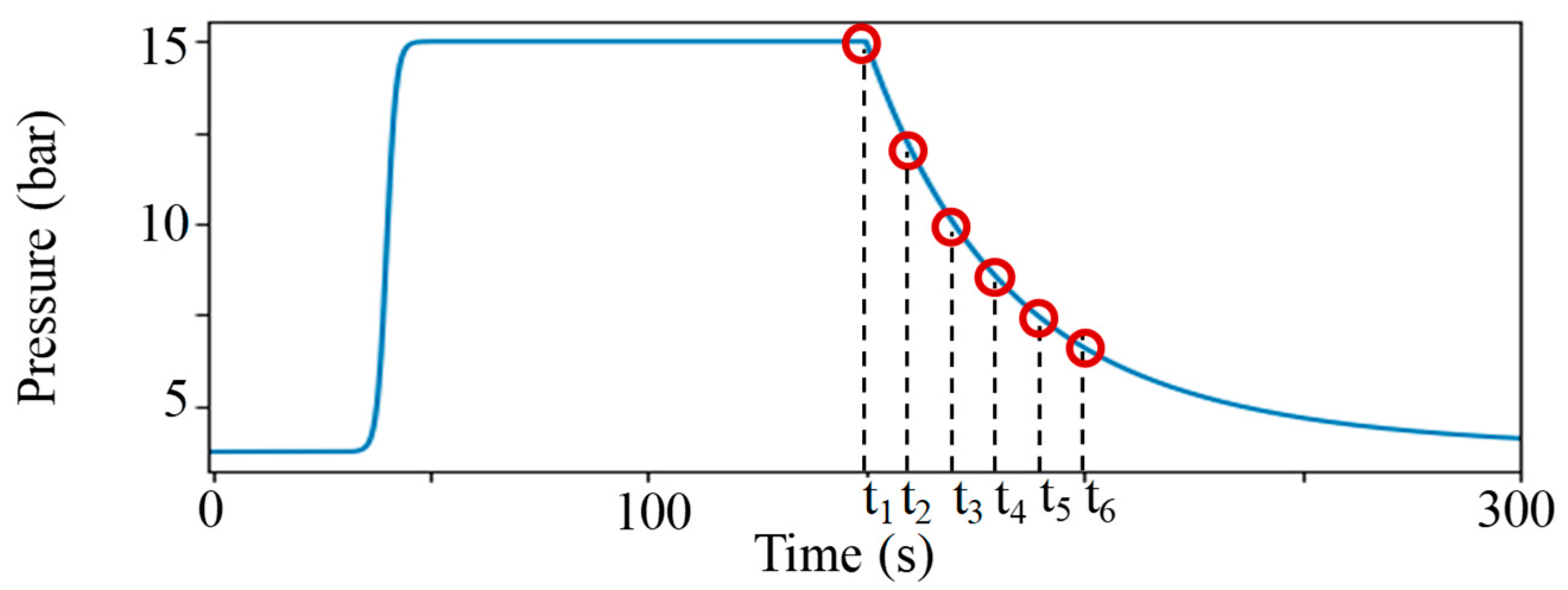
The inlet feed pressure evolution was used to study the local effect in the feed channel along the membrane. The operating conditions are a feed flow rate of about 0.3 L·min⁻¹ and a feed concentration of about 4 g·L⁻¹. As described in Figure 13 and specified in

Table 3. Corresponding times and pressure in the simulation.

Position	Corresponding Time (s)	Pressure (bar)
1	150	15
2	160	12
3	170	9.5
4	180	8
5	190	6.8
6	200	6

, several time positions were chosen to assess the local impacts of the quickly decreasing pressure.

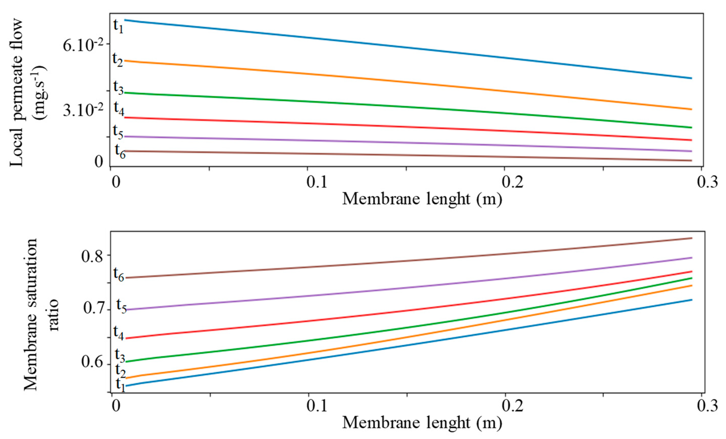
For a better comparison study, a membrane saturation ratio, Sm (Equation (46)) was introduced. It is defined as the ratio between local bulk membrane concentration and the maximum membrane concentration, C_max that would be obtained when the applied trans-membrane pressure equals the osmotic pressure, neglecting the permeate concentration (Equation (47)).

$${\mathrm{S}}_{\mathrm{m}}\left(\mathrm{x},\mathrm{t}\right)=\frac{{\mathrm{C}}_{\mathrm{m}}\left(\mathrm{x},\mathrm{t}\right)}{{\mathrm{C}}_{\max }(\mathrm{x},\mathrm{t})}$$

(47)

$${\mathrm{C}}_{\max }\left(\mathrm{x},\mathrm{t}\right)=\frac{\Delta {\mathrm{P}}_{\mathrm{m}}\left(\mathrm{x},\mathrm{t}\right)}{2\mathsf{\varphi }\frac{{\mathsf{\rho }}_{\mathrm{NaCl}}}{{\widehat{\mathrm{M}}}_{\mathrm{NaCl}}}\mathrm{R}\mathrm{T}}$$

(48)

This saturation ratio can be understood as a saturation degree of the membrane in the channel. When S_m = 1, the maximal concentration is reached regarding the applied pressure; then there is no longer water transfer occurring across the membrane.

Figure 14 shows the local permeate flux and membrane saturation ratio evolutions for six time positions considered during the pressure-decreasing phase (corresponding to the beta phase of the desalination process). This case study enables assessment of the effects of a decreasing feed pressure on local membrane concentration and recovery rates.

From this preliminary study, it can be seen that the influence of a variable applied pressure on membrane wall concentration and the resulting permeate flow is not negligible. A decreasing evolution of the permeate production is observed along the membrane as the membrane concentration rises. Variations of the membrane saturation ratio are more important at the membrane input.

Several cycles are then simulated with a constant solar irradiation applied to the solar collector. Next, the process was simulated over a full day, by considering two data sets of real weather conditions: one sunny and one cloudy.

5.2. Operating and Geometrical Simulation Parameters of the Process

Firstly, size parameters were established to give a scale to the process. These parameters were determined with the aim of an average daily production of desalted water of 500 L·m⁻² of solar collectors from brackish water with a salt concentration of 4 g·L⁻¹. Thermodynamic coefficients were chosen to fit the technical data from selected components. These parameters are summarized in

Table 4. Component sizes of the process and simulation parameters.

Description	Value
Feed tanks volume	3 L
Membrane area	7.2 m²
Solar collectors area	1.5 m²
Linear thermal loss coefficient	3.72 W·m−2·K−1
Quadratic thermal loss coefficient	0.018 W·m−2·K−2
Evaporator exchanger efficiency	0.7
Global Heat transfer coefficient (evaporator)	1000 W·m−2·K−1
Global Heat transfer coefficient (condenser)	1000 W·m−2·K−1
Chemical affinity coefficient (evaporator)	0.8 kg·s−1
Chemical affinity coefficient (condenser)	1.6 kg·s−1
Convection losses coefficient	1 W.K-1
Cylinders mechanical efficiency	0.85

.

Operating conditions were also determined and gathered in

Table 5. Process operating and control conditions.

Description	Value
Working fluid	Sulfur Dioxide (SO2)
Feed water salinity	4 g·L−1
Feed water temperature	18 °C
Ambient temperature	22 °C
Heat transfer fluid mass flow	3.10−2 kg·s−1
Brine flow	2 L·min−1
Beta phase end pressure	8 bars

. Sulfur dioxide was selected as working fluid for its suitable saturation conditions, i.e., it gives high evaporator pressure with a low-grade heat temperature ranging from 50 °C to 80 °C. Feed salt concentration was chosen as typical brackish groundwater and lakes. The final pressure at the beta phase end was chosen to be around a value of 8 bars that maximize clear water production during a cycle.

Controlled brine flow at the outlet of the feed pressure recovery cylinder was determined from the pressure at the end of beta phase and the inlet evaporator power in order to ensure that the main actuator piston had completed its full stroke at the end of each half-cycle.

5.3. Simulations with a Constant Thermal Power Supplied to the Evaporator

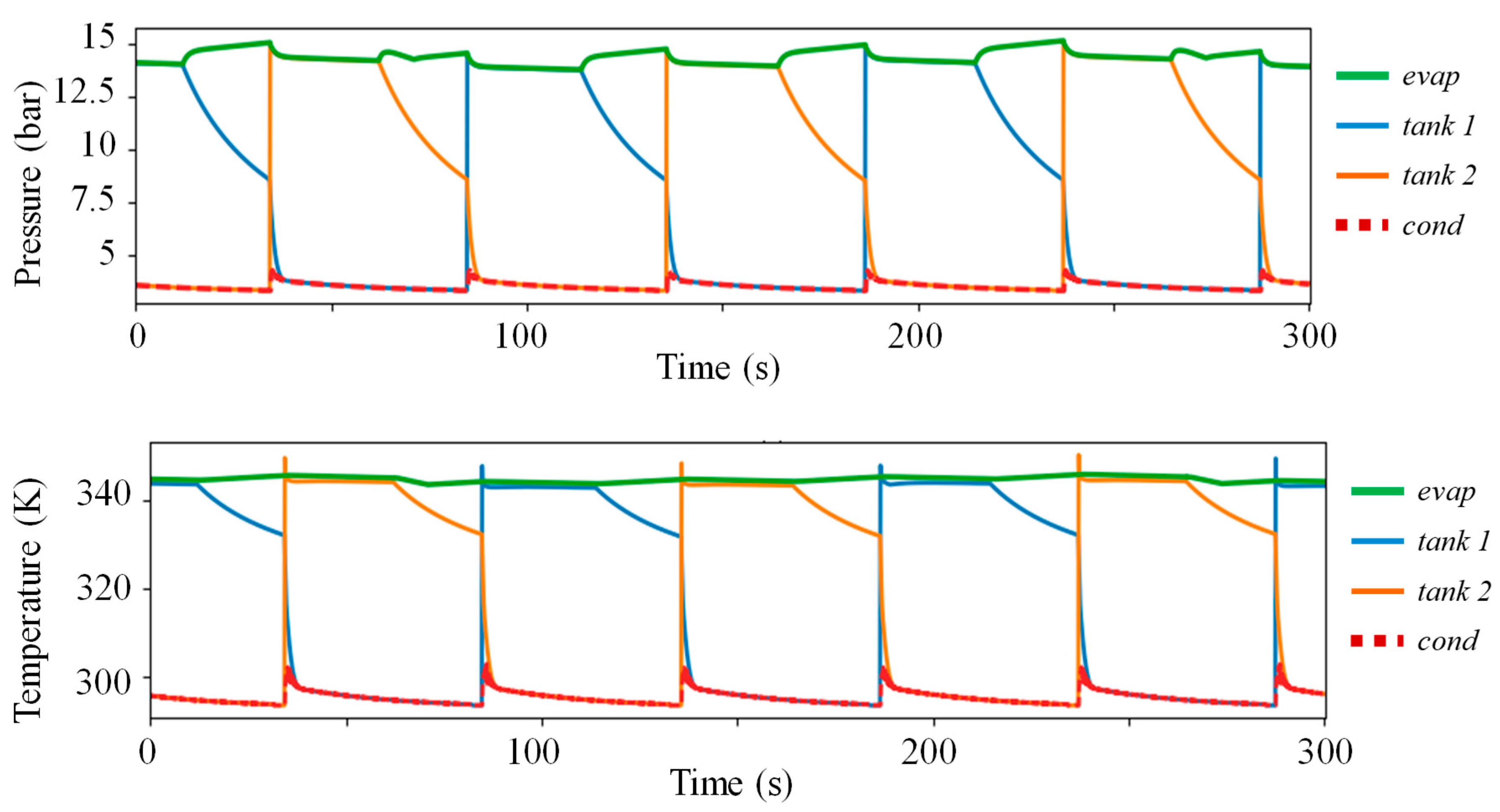
In the first stage, simulations were realized over several cycles with a constant thermal power of 500 W supplied to the evaporator. Figure 15 shows the pressure evolutions in the main components of the process. From this representation, the two main half-cycle phases clearly appear: the alpha phase, where the feed tank is maintained at high pressure, and the beta phase, where its pressure decreases since it is no longer linked to the evaporator. At the beginning of the alpha phase, the second tank is linked to the condenser, so its pressure suddenly drops to reach the condensation pressure. These results show the highly dynamic behavior of the process with half-cycles of about 50 s, shared between the alpha and beta phases. The refilling phase happens each three half-cycles, and can be identified from the pressure drop that occurs in the evaporator during its pressurization, that is, during the beta phase (here at 125 s).

It appears that the evaporator efficiently enables the pressurization of the reservoir to equal to nearly 15 bars, which is a pressure level sufficiently high enough to ensure the RO desalination of the brackish water with a salt concentration ranging from 3 to 8 g·L⁻¹. It also appears that, during the first step, the pressurization is realized at a pressure that is almost constant, which is as expected, taking into account the dimensioning of the evaporator. The condenser pressure evolution shows that the mass flow rate of the pumped feed water is enough to cool it efficiently and maintain a stable condensing pressure. It appears that the temperature and pressure evolutions are similar, and varies between (298 K, 3.5 bars) in the condenser and (340 K, 15 bars) in the evaporator. The temperature of the evaporator and the condenser remains stable over the cycle, whereas the tanks’ ones decrease during the beta phase due to the vapor expansion. When the condenser is connected to the tank, the condenser temperature rises a little and stabilizes quickly.

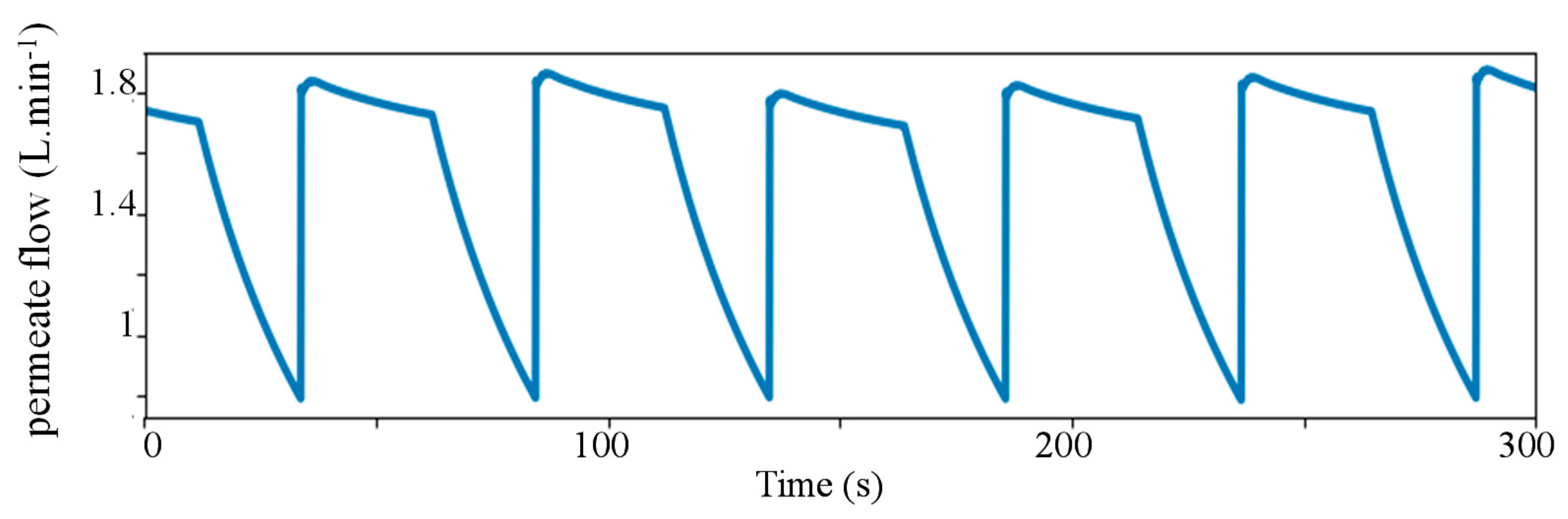
In the permeate production plot presented in Figure 16, the two working phases can also be identified. During the alpha phase, the permeate flow is quite stable even when a slight decrease can be noticed, meaning that the pressure applied to the membrane is unstable, as mentioned before. The decrease during the beta phase is, however, well-pronounced. Nevertheless, this flow decrease never drops to zero because the chosen end-pressure of the beta phase, here being 8 bars, is far beyond the feed-water osmotic pressure (3 bars).

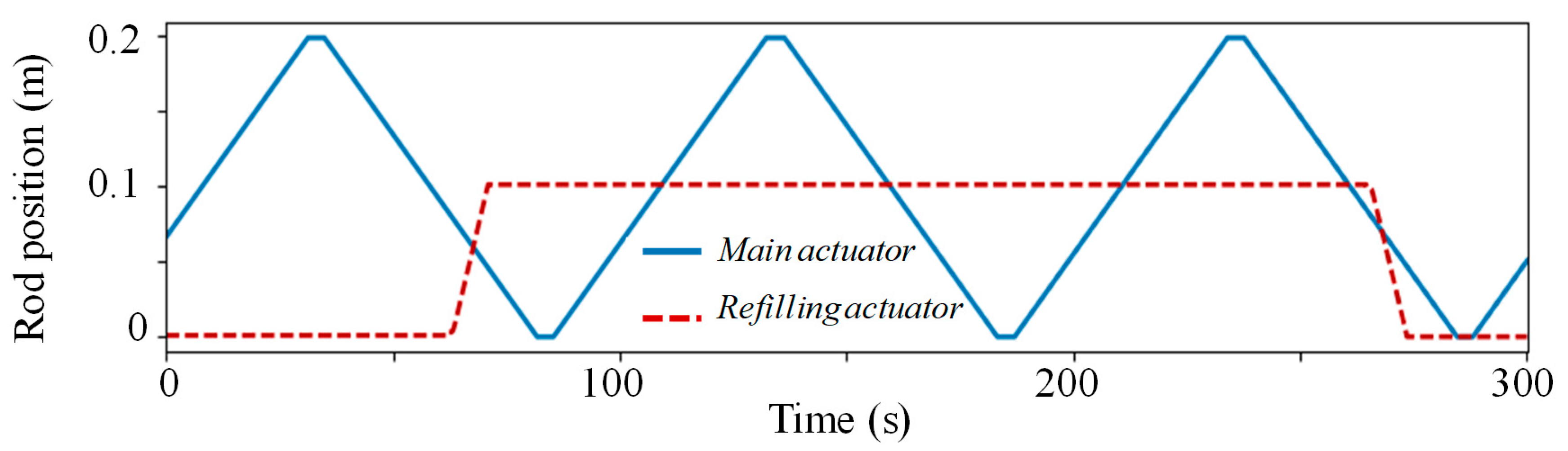
Figure 17 shows the operation of the two actuators and their rods’ positions during the running cycles. The design of these actuators, that is, the piston surface design, has led to consider a total stroke of 0.2 m for the main actuator and 0.1 m for the refilling actuator. The main actuator rod is always in movement, oscillating between its initial position and its end stroke with a constant speed, as the mass flow rate of the brine is controlled and maintained to a constant value. This oscillating movement demonstrates the correct actuator sizing. The other actuator, the refilling one, is activated at every refilling phase, which takes place during a beta phase. It goes until its total stroke is reached, and remains in its position until the next refilling phase, activated by a low liquid level of working fluid in the evaporator.

This first study with a constant power source enables a better understanding of the dynamic of the cycles and offers a comparison between the simulations with the theoretical plots presented in Figure 2. However, there exists a second type of dynamic perturbation, the one linked to the variation of the solar irradiation over the day, that may impact this behavior and the performances of the process. This then needs to be simulated in order to assess the process response over a full day.

5.4. Full-Day Simulation

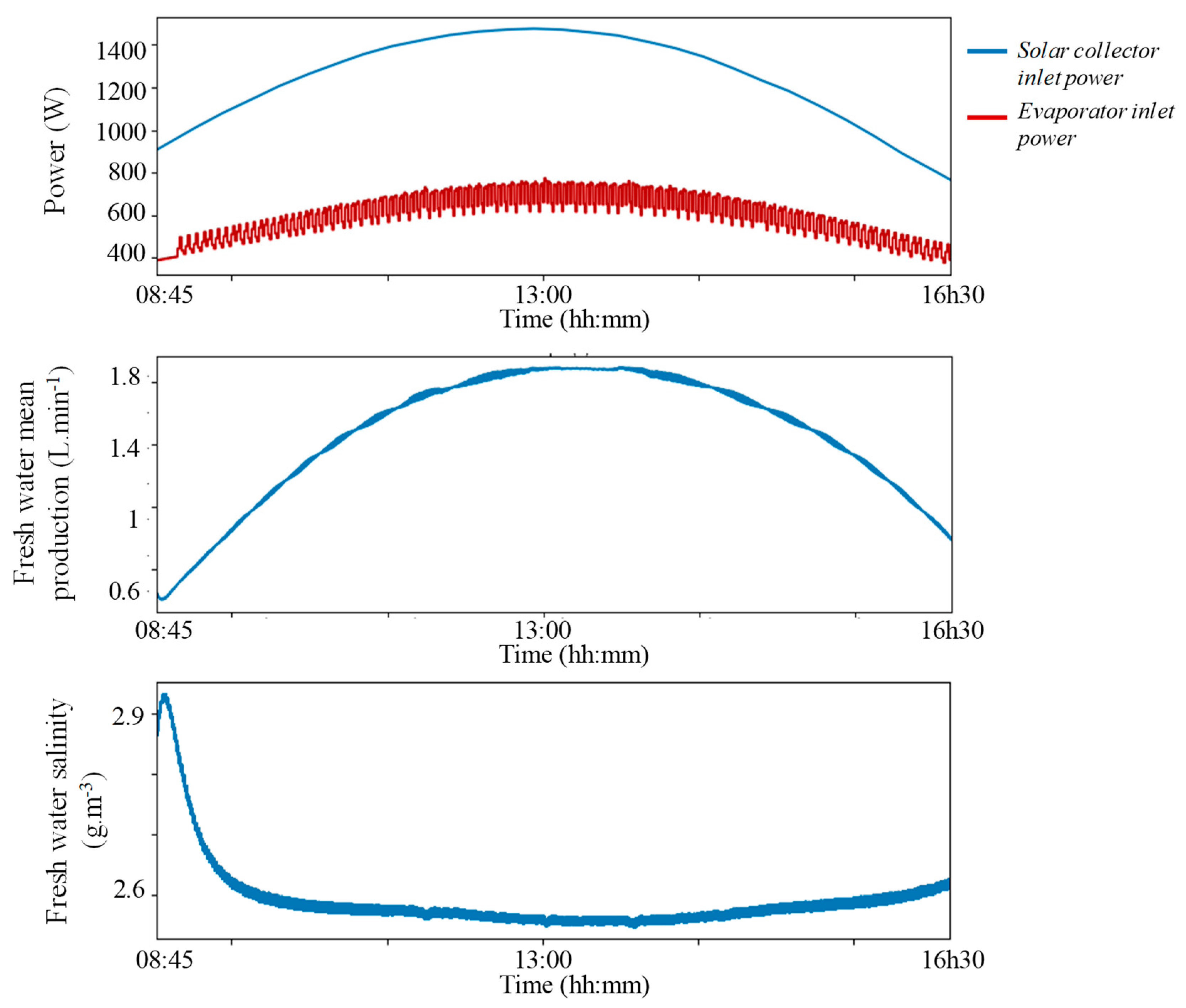
A full-day simulation was thus carried out, and the resulting production and quality of fresh water have been represented aside from the solar irradiation evolution in Figure 18. The data gives the global solar irradiation collected by a solar captor facing south, with an inclination of 40° at the latitude of Perpignan (France). It varies between 550 and 1000 W.m⁻², which corresponds to a power of 800 to 1500 W that is received by the 1.5 m² solar collector and a collected thermal power of 400 to 800 W that is transmitted to the evaporator. This first plot allows for an estimation of the simulated solar collector efficiency of about 50%. The second graph shows the evolution of the permeate flow averaged for each half-cycle during the day, thus demonstrating a trend which clearly correlates with the input thermal power of the system. The obtained recovery ratio of saltwater varies between 30 and 60% during the day. The last plot shows the fresh-water quality over the daily run. The produced water quality is also impacted by the solar power, but its variation is less noteworthy than the permeate production.

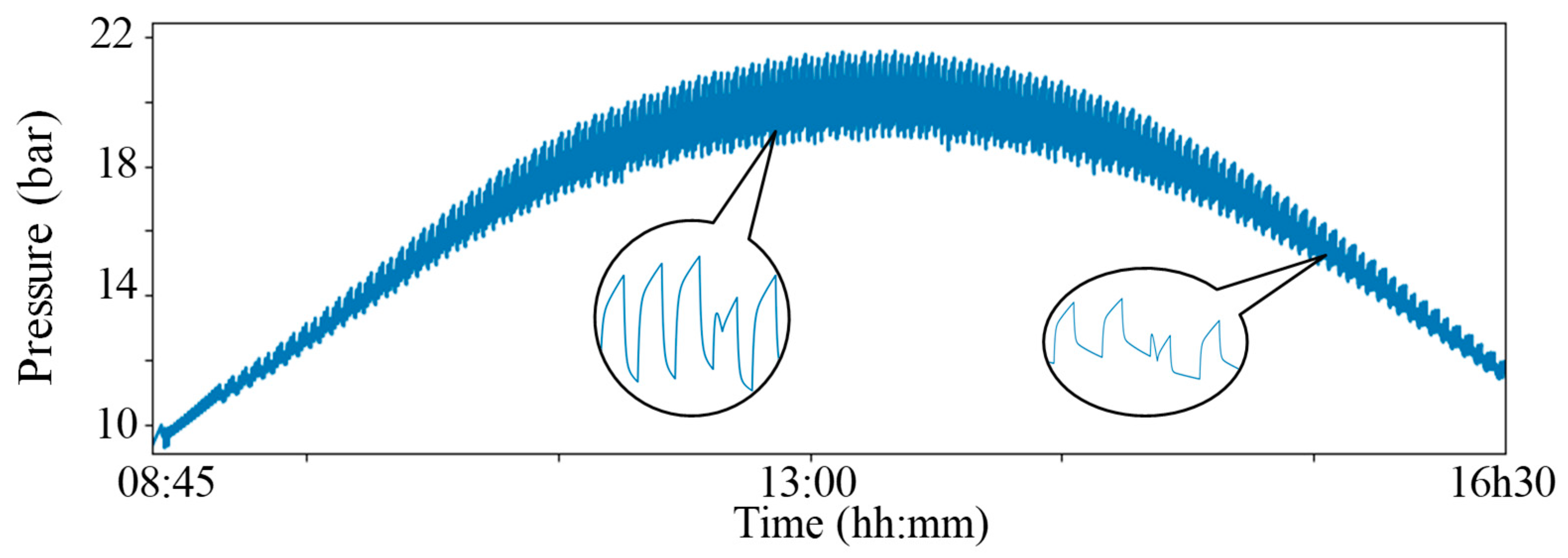
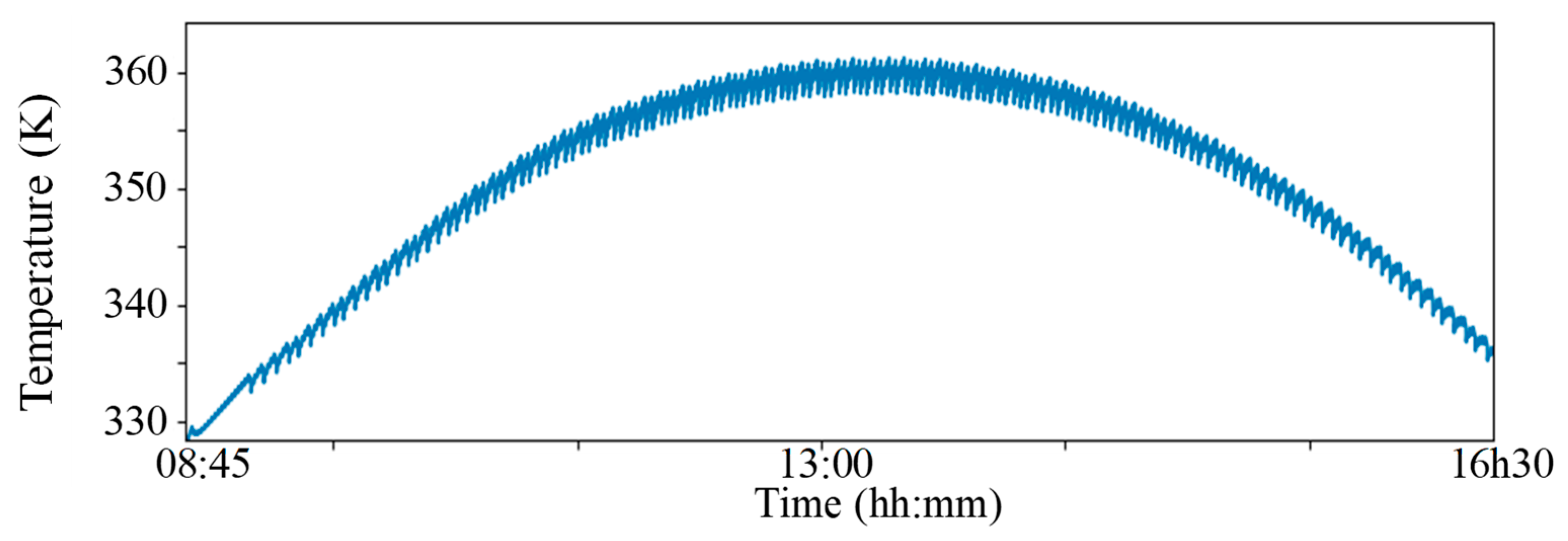
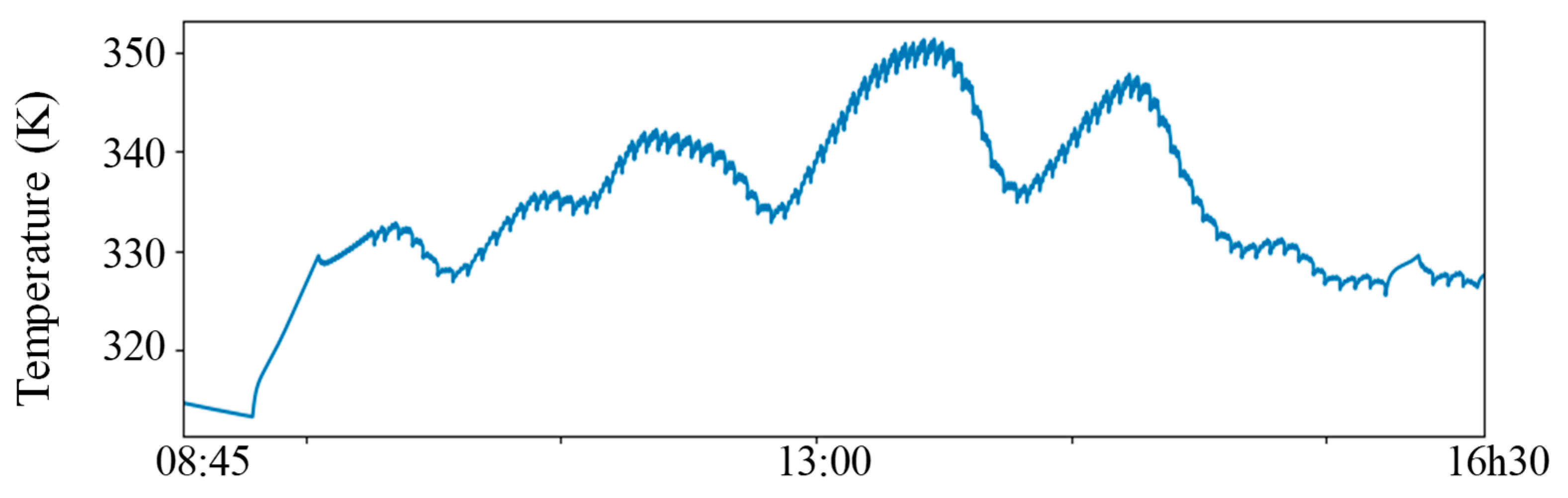
Figure 19 and Figure 20, respectively, show the computed pressure and temperature evolutions of the evaporator over the day. The high pressure varies from 11 to 21 bars, which corresponds to a temperature range from 330 K to 360 K. It can be noticed that the evaporator pressure drop during the alpha phase rises with higher thermal power input. This is due to the increase of the vapor flow across the valve between the evaporator and the transfer tanks.

Such preliminary results allowed us to estimate the daily production of fresh water to 743 L, which corresponds to the community needs of about 5 to 10 families [29]. A salt concentration of around 2.6 mg·L⁻¹ was obtained by this thermo-hydraulic process operating during 136 cycles with 1.5 m² of solar collectors under the climatic conditions of a very sunny day. The specific thermal energy consumption was evaluated to be about 5.8 kWh·m⁻³ of produced fresh water, with daily fresh-water productivity of around 500 L per m² of thermal solar collectors. These performances seem to be competitive in comparison to other solar RO desalination processes that lead to similar energy performances [30,31].

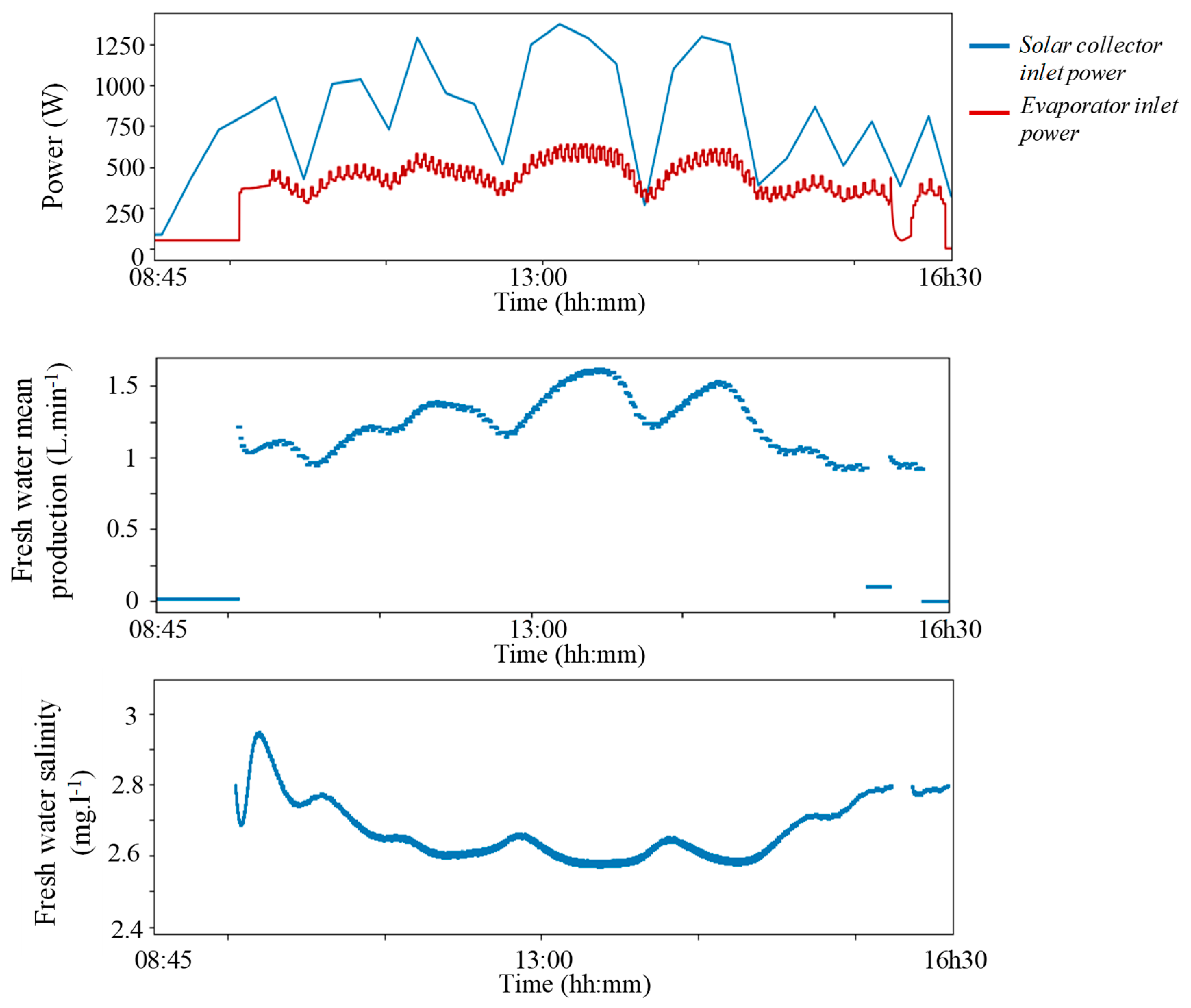
To supplement this performance analysis of the process operating under stable climatic conditions, another simulation has been led considering a highly cloudy day. The results are plotted in Figure 21. This test aims to determine the system reaction to thermal power perturbations at the evaporator. The studied day is disturbed by several cloudy periods, and the irradiation variates between 20 and 900 W·m⁻² with the same daytime duration as the sunny day simulation. The process starts when the evaporator pressure is sufficiently high (approximately 9.5 bars) and operates during almost all of the time period. In Figure 21, the first plot shows solar power that is transmitted to the solar collector and the inlet evaporator power. During the cloudy periods, the evaporator and collector temperatures reach a thermal equilibrium, and then the evaporator inlet power drops to zero. The second plot shows the permeate production averaged over each half-cycle. The permeate flow follows the evaporator power over the day and is rarely null, thanks to the process inertia. The last plot shows the permeate salt concentration that oscillates between 2.5 and 3 mg·L⁻¹, and is higher for low inlet power. Missing points in this plot correspond to the process shutdown period, due to an evaporator pressure that is too low (lower than 9 bars).

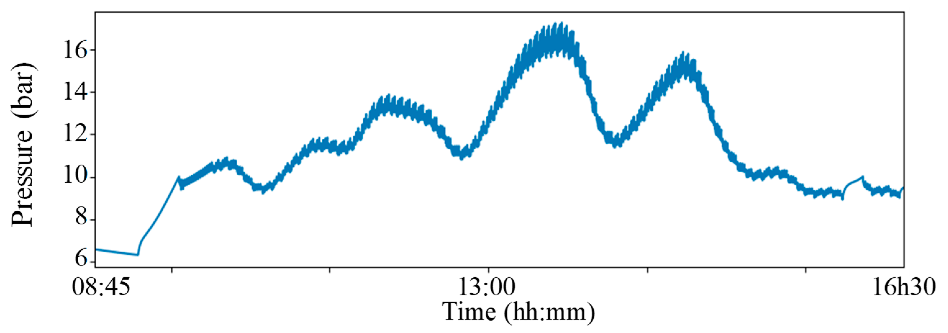
Figure 22 and Figure 23 respectively show the pressure and temperature evolutions in the evaporator simulated over the cloudy day. It can be noticed that the start of the process matches an evaporator temperature of about 325 K and a pressure of about 8.8 bars, and reaches a maximum of 350 K for 16 bars. These plots show that the evaporator is able to supply a pressure that is high enough for operating the RO module and the main cylinder despite the power disturbances, and enables the process to work for almost the entire day.

The results from this second simulation gives a daily production of 275 L with an average quality of about 2.7 mg·L⁻¹ and a specific energy consumption of about 5.67 kWh_th·m⁻³. The water production is much lower on cloudy days due to a lower solar energy input, but the simulation shows that the process inertia allows the production to almost continue over the day despite the disturbances of the source. The operation of the process facing irregular thermal power supply at the evaporator shows that performances could be improved by a continuous control of brine flow and end pressure of the beta phase. This kind of regulation can enable the process to run in the case of low evaporator pressure, and maximize water production during high evaporation pressure periods.

6. Conclusions

Directly powering an RO device by low-temperature heat through an integrated thermodynamic engine cycle without energy storage can lead to drastic reduction of installation, maintenance, and operating costs in comparison to current implemented PV-operated RO desalination plants. The solar-driven thermo-hydraulic process described in this study was designed for these objectives, and can be an interesting alternative for remote populations facing water and energy scarcity, thanks to its autonomous operation and the low cost of the implemented hydraulic and thermal components. This innovative process was presented in this paper, and its working has been described in detail.

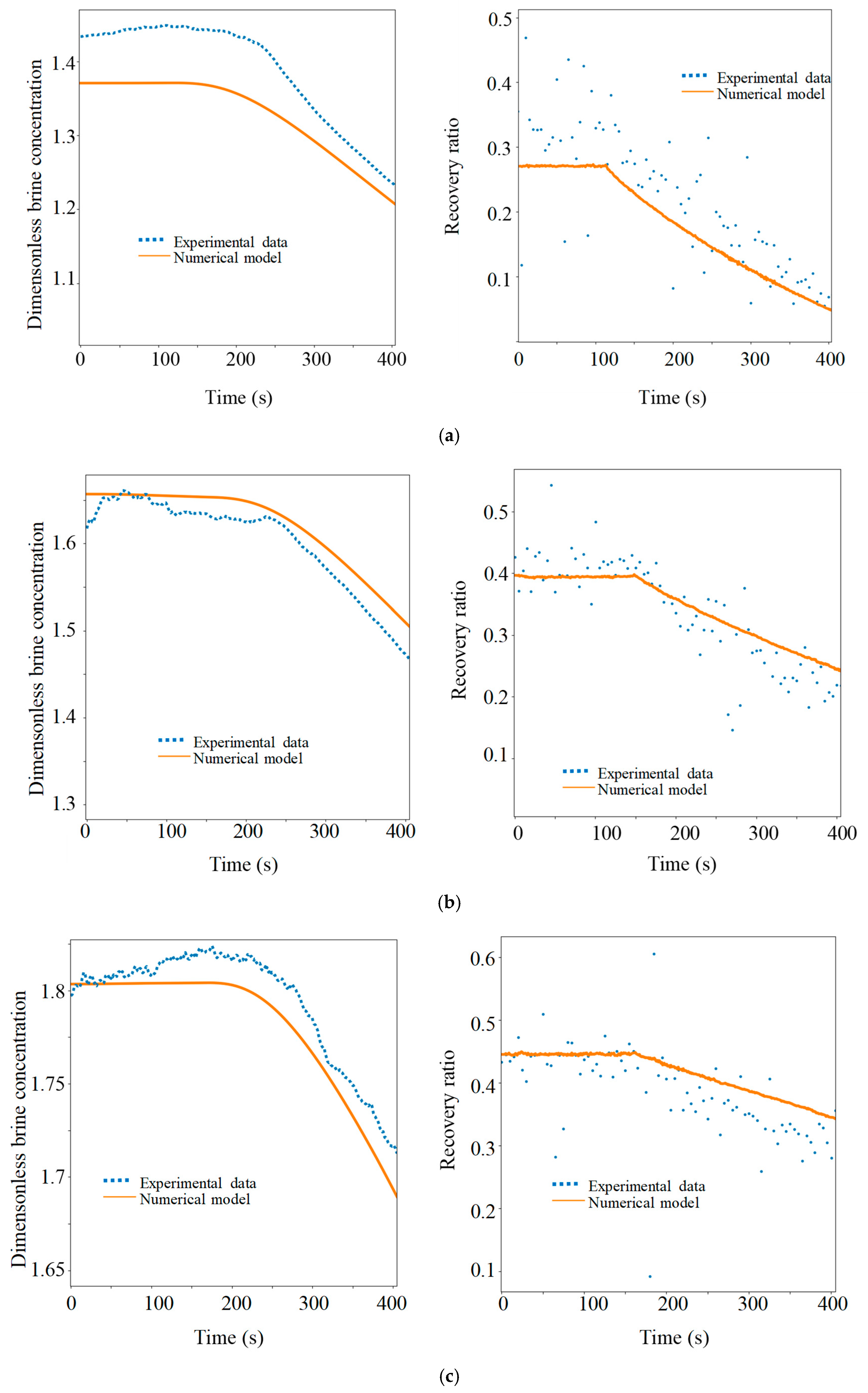
Dynamic modeling of each component of this process has been established considering mass and energy balances under detailed hypothesis. Particular attention has been paid to reverse osmosis membrane modeling, since the dynamic behavior of RO membranes has not been studied much in the literature. An experimental and numerical study on the RO module operating in variable pressure conditions was then presented. An RO membrane adapted for brackish water desalination was experimentally tested under different pressure constraints to calibrate the dynamic model. The evolution of the recovery rate and brine dimensionless concentration obtained by the numerical model matched closely with the experimental one. An analysis of the recovery rate and the saturation ratio along the membrane also showed the high influence of the variability of the feed pressure on the diffusive layer establishment delay, thus impacting the permeate flow across the membrane. This demonstrates that precise dynamic modeling of the RO module is required to take into account the impacts of highly transient running conditions on this innovative, solar, thermally driven RO process.

The simulation of the whole process that has been carried out in this study showed that it is possible to produce approximately 750 L per day from 4 g·L⁻¹ of brackish water by such an installation by only implementing 1.5 m² of solar collectors operating at a low temperature (55 to 85 °C). These preliminary analyses demonstrate that this process may be competitive in comparison to other renewable energy driven desalination systems, especially to PV-RO autonomous processes with SEC of around 2–4 kWh_el·m⁻³ [32,33]. A second simulation was also led in order to assess the process behavior during a cloudy day. The results show that the evaporator inertia minimizes the irradiation perturbation effects and allows for an almost continuous running over the day, but results in lower fresh-water productivity.

The numerical results are promising, but further simulations are necessary to optimize the process working parameters in the aim of lowering the thermal energy consumption, and to improve the process operations facing solar energy variations. A parametrical study also needs to be carried out in order to assess its technical and economical relevancy. An experimental set-up is currently in progress to validate this dynamic modeling and experimentally demonstrate the feasibility of the technical process.

References

1. Ng, K.C.; Thu, K.; Kim, Y.D. Solar-assisted adsorption cycle for the production of cooling effect and potable water. In Proceedings of the 2nd European Conference on Polygeneration, Tarragona, Spain, 30 March–1 April 2011; pp. 1–20. [Google Scholar]
2. Malek, P.; Ortiz, J.; Schulte-Herbrüggen, H. Decentralized desalination of brackish water using an electrodialysis system directly powered by wind energy. Desalination 2016, 377, 54–64. [Google Scholar] [CrossRef]
3. Veza, J.; Peñate, B.; Castellano, F. Electrodialysis desalination designed for off-grid wind energy. Desalination 2004, 160, 211–221. [Google Scholar] [CrossRef]
4. Burn, S.; Hoang, M.; Zarzo, D.; Olewniak, F.; Campos, E.; Bolto, B.; Barron, O. Desalination techniques—A review of the opportunities for desalination in agriculture. Desalination 2015, 364, 2–16. [Google Scholar] [CrossRef]
5. Ali, M.T.; Fath, H.E.; Armstrong, P.R. A comprehensive techno-economical review of indirect solar desalination. Renew. Sustain. Energy Rev. 2011, 15, 4187–4199. [Google Scholar] [CrossRef]
6. Kalogirou, S. Survey of solar desalination systems and system selection. Energy 1997, 22, 69–81. [Google Scholar] [CrossRef]
7. Abutayeh, M.; Li, C.; Goswami, D.Y.; Stefanakos, E.K. Solar Desalination. In Desalination: Water from Water; Scrivener Publishing: Beverly, MA, USA, 2014; pp. 551–581. ISBN 978-1-118-20852-6. [Google Scholar]
8. Thomson, M.; Infield, D. A photovoltaic-powered seawater reverse-osmosis without batteries. Desalination 2002, 153, 1–8. [Google Scholar] [CrossRef]
9. Mascara OSMODEL V1.5. 2015. Available online: https://mascara-nt.fr (accessed on 28 March 2017).
10. Helal, A.; Al-Malek, S.; Al-Katheeri, E. Economic feasibility of alternative designs of a PV-RO desalination unit for remote areas in the United Arab Emirates. Desalination 2008, 221, 1–16. [Google Scholar] [CrossRef]
11. Ghermandi, A.; Messalem, R. Solar-driven desalination with reverse osmosis: The state of the art. Desalin. Water Treat. 2009, 7, 285–296. [Google Scholar] [CrossRef]
12. Pouyfaucon, A.B.; García-Rodríguez, L. Solar thermal-powered desalination: A viable solution for a potential market. Desalination 2018, 435, 60–69. [Google Scholar] [CrossRef]
13. Peñate, B.; García-Rodríguez, L. Seawater reverse osmosis desalination driven by a solar Organic Rankine Cycle: Design and technology assessment for medium capacity range. Desalination 2012, 284, 86–91. [Google Scholar] [CrossRef]
14. Manolakos, D.; Kosmadakis, G.; Kyritsis, S.; Papadakis, G. On site experimental evaluation of a low-temperature solar organic Rankine cycle system for RO desalination. Sol. Energy 2009, 83, 646–656. [Google Scholar] [CrossRef]
15. Igobo, O.N.; Davies, P.A. Isothermal Organic Rankine Cycle (ORC) driving Reverse Osmosis (RO) desalination: Experimental investigation and case study using R245fa working fluid. Appl. Therm. Eng. 2018, 136, 740–746. [Google Scholar] [CrossRef]
16. Nihill, J.; Date, A.; Lappas, P.; Velardo, J. Investigating the prospects of water desalination using a thermal water pump coupled with reverse osmosis membrane. Desalination 2018, 445, 256–265. [Google Scholar] [CrossRef]
17. Dimitriou, E.; Boutikos, P.; Mohamed, E.S.; Koziel, S.; Papadakis, G. Theoretical performance prediction of a reverse osmosis desalination membrane element under variable operating conditions. Desalination 2017, 419, 70–78. [Google Scholar] [CrossRef]
18. Aimar, P.; Bacchin, P.; Maurel, A. Filtration membranaire (OI, NF, UF, MFT) Aspects théoriques: Mécanismes de transfert. Tech. L’ingénieur 2013, 33. ref: J2789 v1. [Google Scholar]
19. Sherwood, T.K.; Brian, P.L.T.; Fisher, R.E. Desalination by reverse osmosis. Ind. Eng. Chem. Fundam. 1967, 6, 2–12. [Google Scholar] [CrossRef]
20. Al-Obaidi, M.; Mujtaba, I. Steady state and dynamic modeling of spiral wound wastewater reverse osmosis process. Comput. Chem. Eng. 2016, 90, 278–299. [Google Scholar] [CrossRef]
21. Rodgers, V.; Sparks, R. Effect of transmembrane pressure pulsing on concentration polarization. J. Membr. Sci. 1992, 68, 149–168. [Google Scholar] [CrossRef]
22. Kim, S.; Hoek, E.M. V Modeling concentration polarization in reverse osmosis processes. Desalination 2005, 186, 111–128. [Google Scholar] [CrossRef]
23. Ali, M.A.-H.; Ajbar, A.; Ali, E.; Alhumaizi, K. Modeling the transient behavior of an experimental reverse osmosis tubular membrane. Desalination 2009, 245, 194–204. [Google Scholar]
24. Cheddie, D.; Maharajh, A.; Ramkhalawan, A.; Persad, P. Transient modeling of wave powered reverse osmosis. Desalination 2010, 260, 153–160. [Google Scholar] [CrossRef]
25. ASCO. Evaluation du Coefficient de Débit et du Diamètre de Passage. Données Tech. pp. 1–6. Available online: http://asco.com (accessed on 4 May 2018).
26. Prigogine, I.; Outer, P.; Herbo, C. Affinity and reaction rate close to equilibrium. J. Phys. Colloid Chem. 1947, 52, 321–331. [Google Scholar] [CrossRef]
27. Lonsdale, H.K.; Merten, U.; Riley, R.L. Transport properties of cellulose acetate osmotic membranes. J. Appl. Polym. Sci. 1965, 9, 1341–1362. [Google Scholar] [CrossRef]
28. Aminot, A.; Kérouel, R. Mesure de la salinité. In Hydrologie des Écosystèmes Marins: Paramètres et Analyses; Editions Quae; 2004; pp. 74–78. Available online: https://books.google.com.hk/books?hl=zh-CN&lr=&id=dd7qZIWQGb8C&oi=fnd&pg=PA9&dq=In+Hydrologie+des+%C3%89cosyst%C3%A8mes+Marins:+Param%C3%A8tres+et+Analyses&ots=4MjXT8A2iu&sig=hU7VGqnZVSoGu79oaT5bfgvpdjA&redir_esc=y&hl=zh-CN&sourceid=cndr#v=onepage&q=In%20Hydrologie%20des%20%C3%89cosyst%C3%A8mes%20Marins%3A%20Param%C3%A8tres%20et%20Analyses&f=false (accessed on 11 September 2019).
29. Jun, Y.-J.; Song, Y.-H.; Park, K.-S. A Study on the Prediction of the Optimum Performance of a Small-Scale Desalination System Using Solar Heat Energy. Energies 2017, 10, 1274. [Google Scholar] [CrossRef]
30. Manolakos, D.; Mohamed, E.S.; Karagiannis, I.; Papadakis, G. Technical and economic comparison between PV-RO system and RO-Solar Rankine system. Case study: Thirasia island. Desalination 2008, 221, 37–46. [Google Scholar] [CrossRef]
31. Cavalcante Júnior, R.G.; Vasconcelos Freitas, M.A.; da Silva, N.F.; de Azevedo Filho, F.R. Sustainable Groundwater Exploitation Aiming at the Reduction of Water Vulnerability in the Brazilian Semi-Arid Region. Energies 2019, 12, 904. [Google Scholar] [CrossRef]
32. Richards, B.S.; Capão, D.P.; Fruh, W.G.; Schäfer, A.I. Renewable energy powered membrane technology: Impact of solar irradiance fluctuations on performance of a brackish water reverse osmosis system. Sep. Purif. Technol. 2015, 156, 379–390. [Google Scholar] [CrossRef]
33. Cheah, S. Photovoltaic Reverse Osmosis Desalination System; Desalination and Water Purification Research and Development Report No. 104; ITN Energy Systems, Inc.: Littleton, CO, USA, 2015. [Google Scholar]
34. Schock, G.; Miquel, A. Mass transfer and pressure loss in spiral wound modules. Desalination 1987, 64, 339–352. [Google Scholar] [CrossRef]
35. Koroneos, C.; Dompros, A.; Roumbas, G. Renewable energy driven desalination systems modelling. J. Clean. Prod. 2007, 15, 449–464. [Google Scholar] [CrossRef]
Figure 1. Global diagram of the thermo-hydraulic desalination process.
Energies 12 04015 g001
Figure 2. Flow diagram of the thermo-hydraulic desalination process during a half-cycle: (a) alpha phase, (b) beta phase, (c) end of half-cycle. Schematic representation of the evolution of the pressure and volume in the transfer tanks, and the mass flow rate of the permeate over one complete cycle.
Energies 12 04015 g002
Figure 3. Flow diagram of the thermo-hydraulic desalination process during the liquid refilling phase of the evaporator by the second cylinder, which is put in motion by the high-pressure vapor supplied by the evaporator during the beta phases of the cycle.
Energies 12 04015 g003
Figure 4. Schematic of evaporator modeling.
Energies 12 04015 g004
Figure 5. Schematic of condenser modeling.
Energies 12 04015 g005
Figure 6. Schematic of transfer tanks modeling during: (a) pressurization, (b) working fluid expansion, and (c) water filling.
Energies 12 04015 g006
Figure 7. Modeling of hydraulic cylinders: (a) main cylinder, (b) refilling cylinder.
Energies 12 04015 g007
Figure 8. Schematic of the reverse osmosis (RO) membrane modeling.
Energies 12 04015 g008
Figure 9. Schematic concentration profile in the half-feed channel in the case of a low (in red line) or a high feed-flow rate (dot line).
Energies 12 04015 g009
Figure 10. Picture (a) and schematic diagram (b) of the experimental setup.
Energies 12 04015 g010
Figure 11. Applied pressure profiles starting at 7, 10, or 12 bars, consisting in a plateau followed by a decreasing evolution.
Energies 12 04015 g011
Figure 12. Comparison of experimental data with the simulated results obtained by the dynamic model for different starting pressures: (a) 7 bars, (b) 10 bars, and (c) 12 bars.
Energies 12 04015 g012
Figure 13. Graph of feed pressure evolution applied to the spiral wound module.
Energies 12 04015 g013
Figure 14. Longitudinal evolution of the local permeate flow and membrane saturation ratio when applied pressure is decreasing.
Energies 12 04015 g014
Figure 15. Simulated temperature and pressure evolutions of the vapor contained in the tanks over several cycles, considering a constant thermal power at the evaporator.
Energies 12 04015 g015
Figure 16. Permeate-simulated flow rate over time, considering a constant thermal power at the evaporator.
Energies 12 04015 g016
Figure 17. Stroke evolutions of the main and refilling actuators over time, considering a constant thermal power at the evaporator.
Energies 12 04015 g017
Figure 18. Simulated fresh-water production and quality over a sunny day.
Energies 12 04015 g018
Figure 19. Simulated evaporator pressure over a sunny day.
Energies 12 04015 g019
Figure 20. Simulated evaporator temperature over a sunny day.
Energies 12 04015 g020
Figure 21. Simulated fresh-water production and quality during a disturbed and cloudy day.
Energies 12 04015 g021
Figure 22. Simulated evaporator pressure during the disturbed day.
Energies 12 04015 g022
Figure 23. Simulated evaporator temperature over the disturbed day.
Energies 12 04015 g023