Article

A New Method of Determination of the Angle of Attack on Rotating Wind Turbine Blades

1
Jiangsu Key Laboratory of Hi-Tech Research for Wind Turbine Design, Nanjing University of Aeronautics and Astronautics, Nanjing 210016, China
2
Department of Wind Energy, Technical University of Denmark, 2800 Lyngby, Denmark
3
School of Hydraulic Energy and Power Engineering, Yangzhou University, Yangzhou 225009, China
*
Authors to whom correspondence should be addressed.
Energies 2019, 12(20), 4012; https://doi.org/10.3390/en12204012
Submission received: 17 September 2019 / Revised: 10 October 2019 / Accepted: 18 October 2019 / Published: 22 October 2019
(This article belongs to the Section A3: Wind, Wave and Tidal Energy)

Abstract

:
The angle of attack (AoA) is the key parameter when extracting the aerodynamic polar from the rotating blade sections of a wind turbine. However, the determination of AoA is not straightforward using computational fluid dynamics (CFD) or measurement. Since the incoming streamlines are bent because of the complex inductions of the rotor, discrepancies exist between various existing determination methods, especially in the tip region. In the present study, flow characteristics in the region near wind turbine blades are analyzed in detail using CFD results of flows past the NREL UAE Phase VI rotor. It is found that the local flow determining AOA changes rapidly in the vicinity of the blade. Based on this finding, the concepts of effective AoA as well as nominal AoA are introduced, leading to a new method of AOA determination. The new method has 5 steps: (1) Find the distributed vortices on the blade surface; (2) select two monitoring points per cross-section close to the aerodynamic center on both pressure and suction sides with an equal distance from the rotor plane; (3) subtract the blade self-induction from the velocity at each monitoring point; (4) average the velocity of the two monitoring points obtained in Step 3; (5) determine the AoA using the velocity obtained in Step 4. Since the monitoring points for the first time can be set very close to the aerodynamic center, leading to an excellent estimation of AoA. The aerodynamic polar extracted through determination of the effective AoA exhibits a consistent regularity for both the mid-board and tip sections, which has never been obtained by the existing determination methods.

Graphical Abstract

1. Introduction

Wind energy has become an important and growing source of electric power. CO2 emission reduction targets and rapidly falling costs per kilowatt-hour have made wind energy the priority option for new power generating capacity in many places of the world. The country with the largest new and total wind power capacities is China (23 GW and 211 GW in 2018, respectively [1]). The region with the highest proportion of wind power in electricity consumption is Europe. In 2018, wind energy covered an estimated 14% of the EU’s annual electricity consumption and a much higher share of 40.8% was achieved in its Member State Denmark [2]. The utilization of wind energy is expected to grow steadily in the future [1], though as a natural energy it still has some unfavorable factors such as unstable output and its related demand for control [3,4].
The great achievements of wind power were driven by the continuous improvement of wind turbine technologies, among which the aerodynamics [5,6,7] is primary. Accurate aerodynamic computation is essential for the design of advanced wind turbines with high power efficiency and low structural loads. There are mainly three general methods in wind turbine aerodynamic computation: the blade-element momentum (BEM) theory [8,9,10], the vortex wake theory (VWT) [11,12], and the computational fluid dynamics (CFD) [13,14]. CFD is the most general one with a minimum of hypotheses, giving the most complete flow information in the whole simulation field. On the other hand, it is the most computationally expensive method. It is meaningful to relate the results of CFD to BEM theory or VWT and validate some key issues such as interference factors [15], tip loss [16,17], rotational effect [18], etc. Many of these investigations highly depend on the determination of the angle of attack (AoA). For example, researchers have to know the AoA in order to compare the lift and drag of a blade section in CFD with those in the BEM theory. However, the determination of AoA in CFD is not straightforward.
Several methods have been introduced for determining AoA using CFD or experimental data. These can be divided into three categories: inverse BEM or VWT, averaging technique (AT), and self-induction subtraction (SIS).
Inverse BEM was developed and used by Snel et al. [19], Bruining et al. [20], Laino et al. [21], Lindenburg [22], and Bak et al. [23], applying the equations of BEM theory to solve the AoA with given forces on blade sections. Inverse VWT was developed by Sant et al. [24,25] and Bretton et al. [26], in which the bound circulation of a free-wake vortex model is computed with section forces by the Kutta–Joukowski law, and AoA is consequently determined from the converged wake structure. An advantage of inverse BEM/VWT is its simplicity: it is easy to convert the normal BEM/VWT code into an inverse one. Nevertheless, the accuracy is restricted to the reliability of BEM/VWT method itself.
The AT method determines AoA by averaging the velocity at multiple locations. Hansen et al. [27] and Johansen et al. [28] performed an annular average along certain rings upstream and downstream of the rotor plane. This is usually called the azimuthal average technical (AAT). The average of Jost et al. [29] is along a symmetric, closed line (usually a circle) around the rotor blade. Rahimi et al. [30] used three monitoring points along the chord length on each side of the rotor. The above two ways of averaging are called the line AT and 3-point AT, respectively. The main function of various types of AT is the same: to cancel out the blade self-induction and estimate the required velocity in rotor plane. Inspired by the idea of cancelling out, Herráez et al. [31] employed only one monitoring point in the rotor plane for each cross-section. The point is located on the bisectrix of the angle between two arbitrary blades where the influence of the self-induction of each blade is cancelled out by the other blades.
Instead of cancelling out blade self-induction, SIS developed by Shen et al. [32,33] directly subtracts self-induction from the velocity of a monitoring point in front of the blade. The Biot–Savart law is used to compute self-induction from the bound circulation. The bound circulation is simplified to a concentrated vortex in [32], which only requires section forces as an input, but leads to a shortcoming that the monitoring point must be kept at a certain distance from the leading edge of the blade. As an improvement, the bound circulation is represented by distributed vortices in [33], which requires the pressure distribution over blade sections as an input. In this situation, the monitoring point can be chosen closer to the blade and a distance between 0.5c to 2.0c (c is the chord length) is recommended. For the sake of simplicity, the technique using a concentrated vortex [32] is hereinafter referred to as SIS1 and that using distributed vortices [33] is referred to as SIS2.
The above methods have played significant roles in the research of wind turbine aerodynamics. The accuracy of BEM method was improved by using the so-called three-dimensional (3-D) lift and drag coefficients extracted through the determined AoA. Such kinds of work were made by Yang et al. [34,35] using SIS1, Schneider et al. [36] using inverse BEM as well as AAT, and Syed Ahmed Kabir et al. [37] using inverse BEM. There exists several other applications with AoA determination, such as improving the actuator line/Navier–Stokes (AL/NS) simulation (Wimshurst et al. [38]), investigating stall delay as well as dynamic stall (Zhu et al. [18]), discussing unsteady phenomena under yawed conditions (Elgammi et al. [39] and Wen et al. [40]), and analyzing the measurements of a wind turbine in the field (Wu et al. [41]). As a key parameter, accurate determination of AoA is of superior importance.
However, discrepancies between the methods were observed by many researchers. In the IEA Task 29 project [42], several methods were attempted to determine the AoA and the corresponding aerodynamic polar of blade sections, including inverse BEM, inverse VWT, and SIS1, but they resulted in remarkable difference (greater than 25%) in lift coefficient for some cases. Guntur et al. [43] observed a discrepancy between inverse BEM and AAT even in the mid-board sections, and attributed it to the effect of trailing vortices. Schneider et al. [36] found that the AoA determined by AAT produced a lower tangential force than the CFD values. Rahimi et al. [30] implemented four different methods of inverse BEM, AAT, 3-point AT, and SIS1. In their results, AAT and SIS1 lead to about 15% lower axial interference factor. Jost et al. [29] analyzed several AT and SIS methods, pointing out that the different considerations of trailing vortices lead to the discrepancies in the tip region. A recent comprehensive evaluation of different methods, including inverse BEM, AAT, line AT, 3-point AT, SIS1, and SIS2, was made by Rahimi et al. [44] on two different 10 MW reference wind turbines. The results are consistent with each other in the mid-board area but discrepancies arise and increase as approaching the tip. In addition, the chosen locations of monitoring points of AT methods were found to be a significant influence on the resulting induced velocity. The above investigations indicate that a deeper understanding of the determination of AoA is still necessary, especially for the tip region.
The present study presents a new method of AoA determination using the CFD velocity field. It combines the advantages of SIS2 and AT methods and determines the effective AoA by five steps: (1) Find the distributed vortices on the blade surface; (2) select two monitoring points per cross-section close to the aerodynamic center on both pressure and suction sides with an equal distance; (3) subtract the blade self-induction from the velocity at the monitoring points; (4) average the velocity obtained in Step 3; (5) determine the AoA using the velocity obtained in Step 4. In addition to the new method itself, the innovation of this study lies in the following items: (a) Based on an analysis of the induction variation in the vicinity of a rotor blade, the definitions of effective AoA and nominal AoA are proposed; (b) effective AoA is found to be different from nominal AoA in the tip region, which to some extent explains the observed discrepancies between the existing methods; (c) the lift and drag coefficients extracted through the effective AoA are largely consistent with those of the 2-D airfoil for both the mid-board and tip sections, which has never been obtained by the existing AT or SIS methods.
The CFD results used in the present study are from the simulations of the NREL UAE Phase Ⅵ rotor [45] solving the Reynolds averaged Navier–Stokes (RANS) equations using the k-ω SST turbulence model. The detailed computational settings and validations can be found in [13].
The paper is organized as follows. In Section 2, an analysis of AoA is made and the concepts of effective AoA and nominal AoA are introduced. In Section 3, the method of computing self-induction is derived. In Section 4, the velocity field after self-induction subtraction is analyzed. In Section 5, the effective AoA is determined by averaging the velocity on two monitoring points adjacent to the aerodynamic center. In Section 6, a comparison is performed between the determined effective AoA and nominal AoA, and the aerodynamic coefficients extracted through them are compared. In Section 7, conclusions of the present study are given.

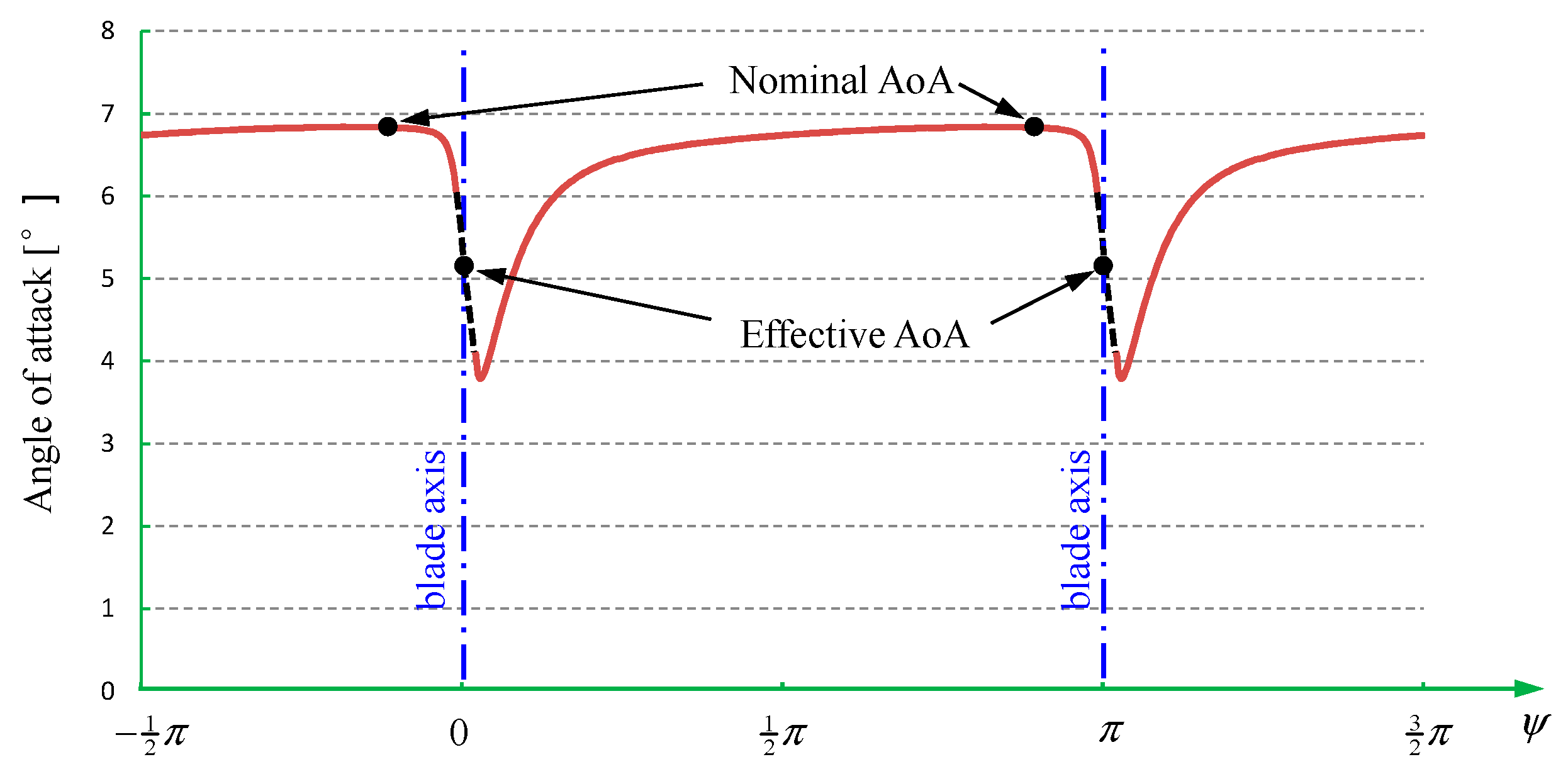
2. Definitions of Effective AoA and Nominal AoA

The classic definition of AoA for a two-dimensional (2-D) airfoil is the angle between the chord line of the airfoil and the undisturbed uniform inflow. The direction of the undisturbed inflow can be obtained by setting a monitoring point far away from the airfoil where the self-induction of the airfoil is negligible. If we have to define the AoA using a monitoring point close to the airfoil, the self-induction at the monitoring point must be subtracted from the measured velocity. In the present paper, self-induction is defined as the velocity induced by the bound circulation of an airfoil/wing/blade.
For a fixed blade with a finite span, an additional induction generated by the tip and root vortices (as well as the trailing vortices before rolling up into the tip and root vortices) arises, which is called tip-root-induction in the present paper. Accordingly, there are two kinds of AoA definition: the geometric AoA and the effective AoA. The geometric AoA is the angle between the local chord and the undisturbed inflow, while the effective AoA is defined by the inflow with tip-root-induction included. The difference between the geometric AoA and the effective AoA of a blade section is an angle determined by the downwash because of the tip-root-induction. It is clear that the effective AoA varies along the wingspan, since the strength of downwash changes at different wing sections.
The inflow experienced by a blade section of a rotor is more complex than described above since the tip and root vortices become helical and there are three kinds of induction. The first induction, which is the azimuthally uniform part of the tip-root induction, corresponds to the induced velocity in which the rotor is simplified to a theoretical disc with an infinite number of blades. It is hereinafter referred to as disc-induction. The second is the blade self-induction. The third is the azimuthally non-uniform part of the tip-root induction, which leads to tip/root loss and is hereinafter referred to as 3D-induction because of its 3-D nature. The disc-induction leads to a continuous increase of the axial interference factor a as well as the tangential inference factor a in the axial direction, causing bended streamlines shown in Figure 1a. In lifting line theory, the most reasonable definition of AoA in this situation should employ the velocity at the aerodynamic center (point C in Figure 1) of the blade section. In practice, however, it is impossible to detect any velocity at the aerodynamic center since it is inside the blade (that is, outside the flow field). As an alternative choice, a monitoring point (point P in Figure 1) in the rotor plane can be set in front of the blade (along the azimuthal direction). The velocity of point P could be regarded to be equal to that of point C (supposing there is a theoretical permeable flow), if the self-induction illustrated in Figure 1b and the downwash (due to 3D-induction) illustrated in Figure 1c were excluded, according to the azimuthally uniform assumption of BEM theory.
Let us think about the effects of the three inductions to the aerodynamic center. The disc-induction and 3D-induction make realistic contributions to the (theoretical) velocity of the aerodynamic center, while the self-induction makes no such a contribution because the aerodynamic center is exactly the center of the bound vortex. Therefore, excluding the self-induction is always necessary for any monitoring point away from the aerodynamic center, but excluding the 3D-induction leads to a different physical meaning of the determined AoA. In the present paper, after the self-induction is subtracted, the AoA defined by the velocity in a certain front of a blade section (where the 3D-induction is negligible) is called the nominal AoA, while the AoA defined at the aerodynamic center is called the effective AoA.
The existing methods of AoA determination lead to AoA with different physical meanings. The inverse BEM (with a tip / root loss correction) or inverse VWT method determines the velocity at the blade axis (which usually is very close to, even coincident with, the aerodynamic center), leading to an estimation of effective AoA. The AAT method estimates the annularly averaged velocity in the rotor plane, which significantly weakens the effect of 3D-induction and thus results in an AoA close to the nominal AoA. The line AT and 3-point AT methods attempt to estimate the velocity of the aerodynamic center but their monitoring points have to be kept within a certain distance (usually about 1 chord length) from the aerodynamic center, leading to a blend of effective AoA and nominal AoA. The SIS1 and SIS2 methods employ a monitoring point in front of the blade where the 3D-induction is small and thus results in a nominal AoA.
The methods as well as their corresponding kinds of determined AoA are listed in Table 1. It is obvious that different methods should be employed for different purposes, depending on which kind of AoA is required. For the blade sections of mid-board, the effect of 3D-induction is usually small and thus the nominal AoA and the effective AoA tend to be consistent.

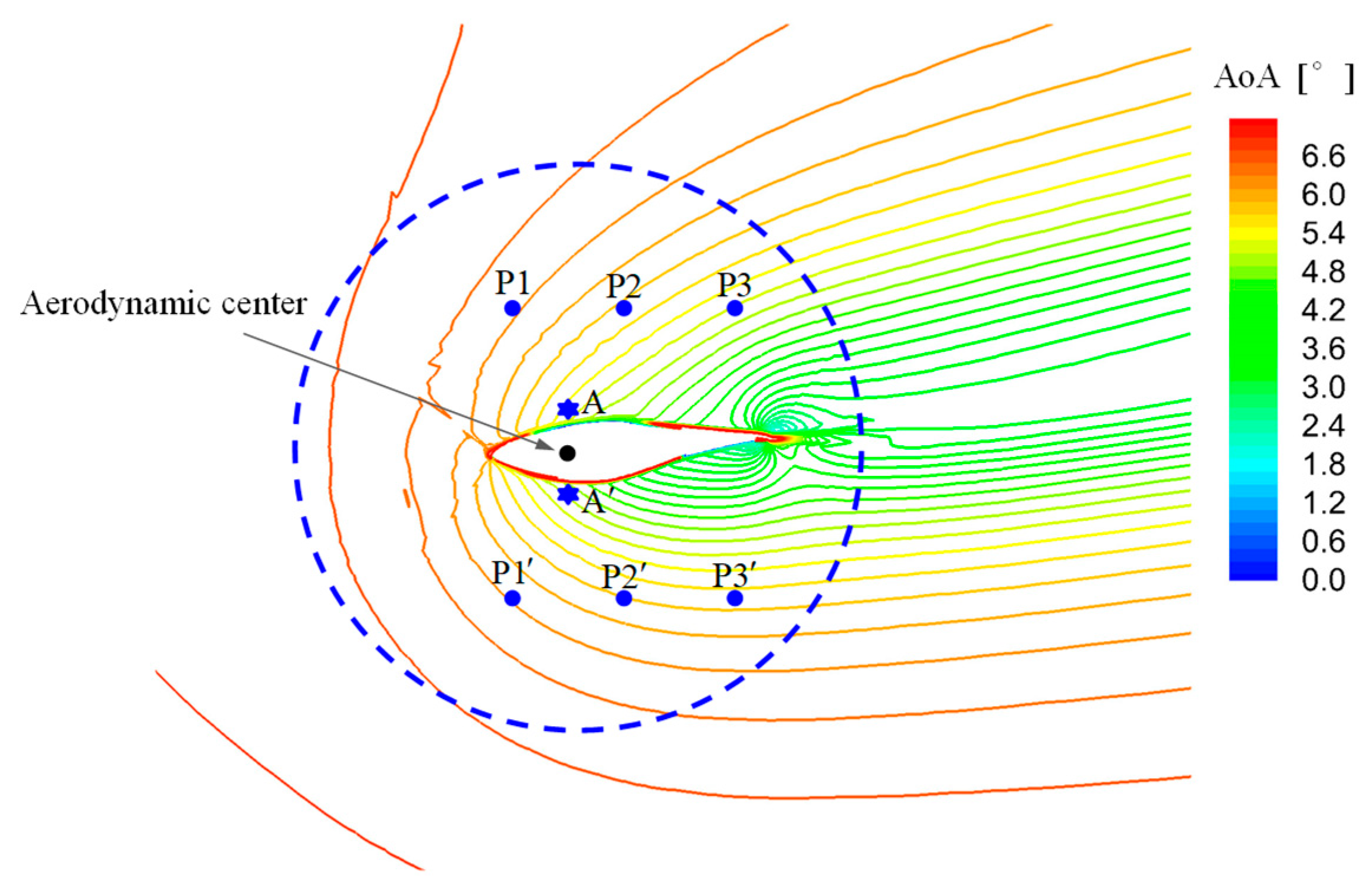
3. Method of Computing Self-Induction

3.1. Representing Airfoil by Distributed Vortices

According to the Kutta–Joukowski law, the lift of an airfoil in a potential flow can be related to a bound circulation of the airfoil by
L = ρ V Γ
where L is lift, ρ is air density, V is inflow speed, and Γ is the circulation of a concentrated vortex which typically is located at the quarter chord point of the airfoil. The concentrated vortex of an airfoil at a positive AoA is illustrated in Figure 2. The circulation is defined as positive when the induced velocity of the vortex is clockwise in the present paper, meaning that the illustrated circulation is positive and leads to a positive lift according to Equation (1). A shortcoming of representing the airfoil by a concentrated vortex is that the induced velocity of the vortex, e.g. v at a point P(x,y) in Figure 2, is different from that of the airfoil entity in the near field, because of the ignorance of the airfoil’s geometry.
Another choice is to properly distribute vortices over the airfoil, as illustrated in Figure 3a. The vortex distribution needs to meet two requirements. First, the sum of the circulations of the distributed vortices should be equal to the circulation of the concentrated vortex,
Γ = k = 1 n γ k
where γ k is the circulation of the kth vortex, and n is the total number of the distributed vortices. Second, at any point P(x,y), the velocity induced by the distributed vortices should be consistent with that induced by the airfoil entity,
v v o r t i c e s ( x , y ) = v a i r f o i l ( x , y )
The above two conditions will be met only when γ k is determined by the actual velocity distribution over the airfoil.
In order to determine γ k , the airfoil surface is divided into n small segments, each corresponding to one of the distributed vortices. Figure 3b illustrates the viscous boundary-layer flow on the kth small segment. The definition of circulation leads to
γ k = A B v d s + B C v d s + C D v d s + D A v d s
where d s is a microelement along the clockwise and closed circuit A-B-C-D-A, and v is the corresponding local velocity. The segment BC is located on the edge of the boundary-layer. According to the boundary-layer theory [46], the velocity along DA (on the wall) is zero, and the velocity on AB or CD is almost perpendicular to the segment itself. As a result, the integrations along the segments AB, CD, and DA are zero, and the equation becomes
γ k = B C v d s v k l k
where v k is the averaged velocity on BC, and l k is a vector pointing from B to C with | l k | = B C = A D
Although the velocity at any location in the flow field can be obtained from CFD simulations, | v k | is difficult to be directly determined because the thickness of boundary-layer varies along the airfoil surface. Instead of calculating the thickness of boundary layer, Shen et al. [33] suggested determining v k from the local pressure by applying the Bernoulli equation. For an airfoil with fully attached flow, the viscous effect is substantially limited within the boundary-layer that is usually very thin. Therefore, the Bernoulli equation can be regarded as valid outside the boundary-layer, giving the relation between the velocity and pressure,
p + 1 2 ρ V 2 = p k + 1 2 ρ | v k | 2
or
| v k | = V 2 2 ( p k p ) ρ
where p k is the pressure at the location of the kth vortex, which can be taken from the airfoil surface since pressure is almost unchanged across the boundary-layer.
The circulation of the kth vortex, γ k , can now be determined by Equations (5) and (7). The filaments of the distributed vortices can be regarded infinitely long in the direction perpendicular to the plane of the airfoil, since the concept of airfoil is 2-D. The induced velocity at any point P(x,y) can then be computed by the following formula according to the Biot–Savart law for infinitely long vortex filaments,
v v o r t i c e s ( x , y ) = k = 1 n γ k 2 π | r k | 2 ( e × r k )
where r k is the vector pointing from the kth vortex to point P ( x , y ) , and e is the unit vector in the direction of the vortex (perpendicular to the airfoil plane and points inside in Figure 2.
The velocity field around the airfoil can now be reproduced by the distributed vortices, through a simple summation of
v v o r t i c e s ( x , y ) = V + v v o r t i c e s ( x , y )
In order to evaluate the method introduced above, | v a i r f o i l | / V is compared with | v a i r f o i l | / V in Figure 4, where | v a i r f o i l | is the induced velocity of the airfoil entity,
v a i r f o i l ( x , y ) = v ( x , y ) V
in which v ( x , y ) is the velocity at point P(x,y), obtained from CFD in the present paper. As shown in Figure 4, the two contour maps look largely similar to each other. There is no difference observed except in a slender region of the viscous wake originated from the trailing edge. The vortices give a result with no viscous wake because of the potential assumption.
A relative error can further be defined as
δ = | v v o r t i c e s v a i r f o i l | V × 100 %
which is contoured in Figure 5. It is observed that: (1) The relative error is generally small in the flow domain, and can be considered negligible ( δ < 0.5 % ) beyond a certain distance from the airfoil; (2) the error is negligible in the region close to the front half of the upper surface of the airfoil; (3) the error increases as approaching the trailing edge, but is almost less than 5% except in the viscous wake.
In general, the results shown in Figure 4 and Figure 5 indicate a good representation of the airfoil entity by the distributed vortices.

3.2. Representing Blade by Distributed Vortices

As in the airfoil case, a blade can also be represented by bound vortices distributed over its surface. Part of a rotor blade is illustrated in Figure 6 where the surface is divided into small faces. Supposing that the pressure distributions of the two neighboring blade sections (Section 1 and Section 2 in Figure 6) are known, the bound vortices between the two sections can be determined.
Let us consider a small face ABCD in Figure 6, which is indexed as the kth face in the next derivation. Points A and B are located at the equal dimensionless locations on their respective sections, as well as points C and D. The vortex of this face can be simplified to a line vortex starting from point P1(x1,y1,z1) and ending at point P2(x2,y2,z2) if the lengths of AD and BC are small enough. Points P1 and P2 are the midpoints of AD and BC, respectively.
In a rotational reference frame fixed with the rotor, supposing the pressure values of points P1 and P2 are known, the Bernoulli equation leads to
p + 1 2 ρ ( V 2 + ω 2 r S 1 2 ) = p 1 + 1 2 ρ | v 1 | 2
p + 1 2 ρ ( V 2 + ω 2 r S 2 2 ) = p 2 + 1 2 ρ | v 2 | 2
resulting in
| v 1 | = V 2 + ω 2 r S 1 2 2 ( p 1 p ) ρ
| v 2 | = V 2 + ω 2 r S 2 2 2 ( p 2 p ) ρ
where v 1 and v 2 are the velocity of points P1 and P2, respectively; p 1 and p 2 are the pressure of the points P1 and P2, respectively; r S 1 and r S 2 are the radial location of the Section 1 and Section 2, respectively. The circulation of the line vortex can then be estimated by the following average:
γ k = 1 2 ( v 1 A D + v 2 B C )
where A D and B C are the path vectors ( | A D | = A D , | B C | = B C , the vector directions are consistent with the clockwise direction in Figure 6).
At point P(x,y,z) in the flow domain, the velocity induced by the kth line vortex can then be determined by the Biot–Savart law,
v k = γ k 4 π r 1 × r 2 | r 1 × r 2 | 2 ( r 1 r 12 | r 1 | r 2 r 12 | r 2 | )
in which
r 1 = ( x x 1 ) i + ( y y 1 ) j + ( z z 1 ) k
r 2 = ( x x 2 ) i + ( y y 2 ) j + ( z z 2 ) k
r 12 = ( x 2 x 1 ) i + ( y 2 y 1 ) j + ( z 2 z 1 ) k
and i , j , k are unit vectors in the x, y, z directions.
The velocity induced by all the distributed vortices can be computed by a summation,
ν v o r t i c e s ( x , y , z ) = i = 1 B k = 1 n v k
where B is the number of rotor blades, and n is the number of small faces on each blade. ν v o r t i c e s ( x , y , z ) is exactly the blade self-induction. It is clear that the result will be more accurate if the faces are smaller.

4. Subtraction of Blade Self-Induction

One basic assumption of BEM theory is that the flow remains uniform in the azimuthal direction. However, this assumption cannot be directly validated by the velocity field simulated by CFD, because of the existence of the blade self-induction. Taking a mid-board section of r/R = 47% as an example, Figure 7 shows the contours of axial interference factor defined by using a CFD velocity field before the self-induction is subtracted. It is clearly shown that a strong variation exists around the blade, which is obviously far from the azimuthally uniform assumption of BEM theory and can only be caused by the blade self-induction. In order to make the CFD and BEM results comparable, the blade self-induction must be subtracted.
The method of representing the blade entity by distributed vortices provides a way for subtracting the blade self-induction. The velocity after the subtraction, denoted by v ˜ , can be computed by:
v ˜ ( x , y , z ) = v ( x , y , z ) ν v o r t i c e s ( x , y , z )
The axial interference factor defined by the velocity v ˜ is shown in Figure 8. The thick dashed line represents the rotor plane with many fewer contours than that in Figure 7, implying much less variation in the azimuthal direction.
The azimuthal ( ψ ) variation of axial interference factor in the rotor plane is plotted in Figure 9, with the results before and after the self-induction subtraction. In front of the blade (left of the blade axis), the curve of “After subtraction” is approximately horizontal in a wide range of azimuthal angle, while the curve of “Before subtraction” presents a significant decline. Obviously, the result of “After subtraction,” rather than that of “Before subtraction,” is comparable with the BEM theory. As for the sharp fluctuation behind the blade (right of the blade axis), it is a result of the viscous effect of trailing wake.

5. Determination of Effective AoA

Figure 10 shows the contours of axial interference factor in the flattened section of r/R = 95%, defined by the velocity after the self-induction subtraction. The 3D-induction dominates the flow field of this tip section, which is very different from the result of r/R = 47% (Figure 8). Figure 11 shows the local perspectives of the two sections. In the r/R = 47% section, the influence of viscous trailing wake is limited to an area after the trailing edge. In the r/R = 95% section, the 3D-induction covers the whole blade section including the aerodynamic center, implying a significant influence of the effective AoA.
The 3D-induction causes an azimuthally non-uniform flow in the rotor plane, leading to a dependence of the determined AoA on the locations of monitoring points. Figure 12 illustrates the definition of nominal AoA and effective AoA. If the AoA is determined at a monitoring point that is a certain distance in front of the blade, it should be regarded as nominal AoA. The closer the monitoring point is to the aerodynamic center the closer the determined AoA is to the effective AoA. However, it is never possible to get an exact effective AoA since no velocity can be detected if the monitoring point is placed inside the blade.
A technique has to be introduced to estimate the virtual velocity at the aerodynamic center, if the effective AoA needs to be determined. The contours of AoA determined by the local velocity (after the self-induction subtraction) are shown in Figure 13. The monitoring points of the 3-point AT and the monitoring circle of the Line AT are also illustrated. It is clear that the determination would be more accurate if the monitoring points (circle) were closer to the airfoil. However, the two techniques have to be set at a certain distance between the monitoring points (circle) and the blade in order to avoid the error introduced by the blade self-induction, because no self-induction subtraction was performed. Once the blade self-induction is subtracted, much closer monitoring points can be set.
In the present determination, two monitoring points (A and A’ in Figure 13) are set adjacent to the airfoil surface, being above and below the aerodynamic center and with a same distance to the rotor plane, respectively. In the present study, the aerodynamic center is assumed to be at the 25% chord and the specific locations of the points A and A’ are defined as: their azimuthal coordinates are identical and are equal to that of the 25% chord, and their axial distances from the rotor plane are also identical and are determined by a minimum range covering the inside area and the boundary-layer (which can be easily identified by the velocity contours) of the blade. The two locations are very close to the aerodynamic center and thus can be expected as the best choice for determining the effective AoA. The final determined effective AoA is
α e = arctan ( v ˜ a ( A ) + v ˜ a ( A ) v ˜ t ( A ) + v ˜ t ( A ) ) θ
where v ˜ a and v ˜ t are the axial and tangential velocity after the self-induction subtraction.
To summarize, the new method of determination of AOA has five steps: (1) Find the distributed vortices on the blade surface (Section 3); (2) select two monitoring points per cross-section close to the aerodynamic center on both pressure and suction sides with an equal distance from the rotor plane; (3) subtract the blade induction from the velocity at each monitoring point (Section 4); (4) average the velocity of the two monitoring points obtained in Step 3; (5) determine the AoA using the velocity obtained in Step 4 (Equation (20)).

6. Comparison and Validation

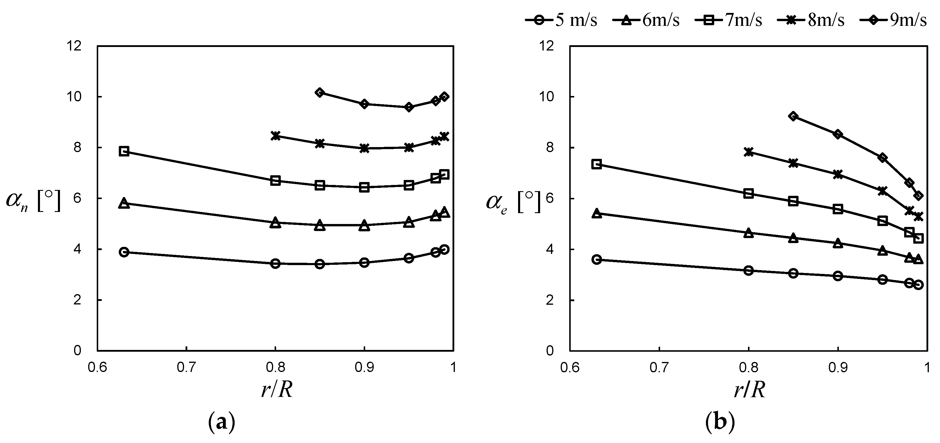
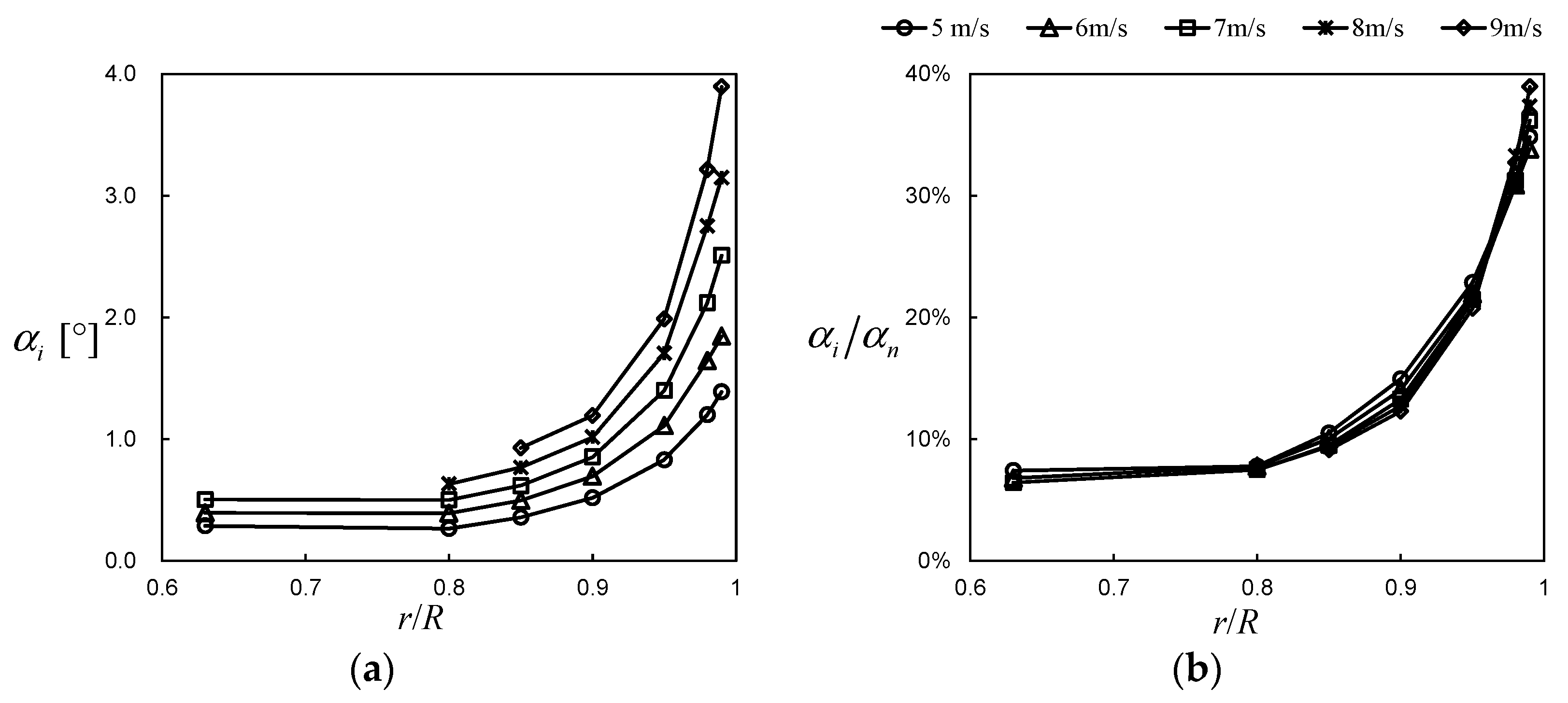
6.1. Comparison Between Nominal AoA and Effective AoA

A comparison between the nominal AoA ( α n ) and the effective AoA ( α e ) is shown in Figure 14. The nominal AoA is determined by setting a monitoring point in the 0.5c front of the blade in the velocity field after the self-induction subtraction. From the mid-board to the tip, the nominal AoA goes down first and then goes up, while the effective AoA presents a downward trend and drops faster in the tip region. This result answers the question raised from the existing evaluations [43,44]; why different AoA determination methods lead to different trends in the tip region. The reason is that different determinations may lead to different definitions of AoA (nominal, effective, or blended).
The difference between the nominal AoA and the effective AoA is the induced angle because of downwash which is called downwash angle in the present paper,
α i = α n α e
The trend of α i along r/R is shown in Figure 15a. The curves rise faster as r/R approaches the tip. In addition, a higher wind speed leads to a larger value of α i at a certain location of r/R. The ratio of α i to α n , which is shown in Figure 15b, looks interesting: all the curves generally coincide with each other. That implies a rule exists in the relationship between α i and α n . The value of α i might be estimated from α n that can be more easily determined, if a model of their relationship could be established in the future work.

6.2. Validation of Extracted Lift and Drag Coefficients

As AoA is determined, the lift and drag coefficients of blade elements can be extracted through the following relation,
C l = C n cos ϕ C t sin ϕ
C d = C n sin ϕ C t cos ϕ
in which ϕ = α + θ is the flow angle, C n and C t are the normal and tangential force coefficients determined by
C n = F n 1 2 ρ V r e l 2 c
C t = F t 1 2 ρ V r e l 2 c
where F n and F t are the normal and tangential forces of the blade section, and V r e l is the relative velocity.
Figure 16a,b shows the lift coefficients extracted through α n and α e , respectively. The forces used to determine the coefficients are obtained from pressure integration over the airfoil/blade sections. The 2-D experimental data [47] and 2-D CFD data are for the airfoil S809 at Reynolds number of 1 × 10 6 . Remarkable differences between C l ( α n ) and C l ( α e ) are seen. For the sections of r/R = 63% and r/R = 85%, the curves of C l ( α n ) is slightly lower than the 2-D experimental/CFD data, while the curves of C l ( α e ) are in good agreement with each other as well as the 2-D experimental/CFD data. For the sections closer to the tip (r/R = 95% and r/R = 99%), the curves of C l ( α n ) are observed to decline significantly, being far away from the 2-D data. In contrast, the curves of C l ( α e ) do not show a sustained decline. The curves of r/R = 95% and r/R = 99% are consistent with each other. They are only slightly lower than the 2-D curves, which could be caused by some phenomena, e.g., the de-cambering effect [48], which are not taken into account in the present study.
Figure 17a,b shows the drag coefficients corresponding to α n and α e , respectively. The curves of C d ( α n ) are observed much higher than the 2-D experimental/CFD data. In contrast, the curves of C d ( α e ) match much better with each other and the 2-D experimental/CFD data, except the curve of r/R = 99%. The exception implies some physical difference in the mechanism of drag between the section of extreme tip and the 2-D airfoil.
The above results have definitely shown that the lift and drag coefficients extracted through the effective AoA are largely consistent with those of the 2-D airfoil for both the mid-board and tip sections. This regularity of consistence has never been obtained by existing AT or SIS methods.

7. Conclusions

A new method has been developed and presented for determining the AoA of rotating wind turbine blades. For AT methods, there must be a sufficient distance between the monitoring points and the blade in order to avoid the errors caused by the blade self-induction. The present method completely overcomes this shortcoming by representing the blade entity with distributed vortices and subtracting their induction from the velocity at monitoring points. The monitoring points are for the first time set very close to the aerodynamic center of the blade, leading to an excellent estimation of the effective AoA. The success of this method is based on a combination of the advantages of the SIS2 and AT methods. The method may be regarded as an extension of the SIS2, and thus can be called SIS3. The following conclusions are drawn from the present study:
  • The determination of AoA depends on the consideration of different inductions (disc-induction, blade self-induction, and 3D-induction) experienced by the rotor blade. The blade self-induction should always be excluded, disc–induction leads to the nominal AoA, and the sum of disc-induction and 3D-induction, i.e., the tip-root-induction, leads to the effective AoA. The discrepancies between existing methods observed by other researchers are to some extent caused by the unclassified comparisons.
  • The effective AoA and the nominal AoA are close to each other at mid-board sections but have different trends when approaching the tip. From the mid-board to the tip of the studied rotor, nominal AoA decreases first and then increases, while the effective AoA presents a downward trend and drops faster in the tip region.
  • The difference between the nominal AoA and the effective AoA is the downwash angle. The ratio of the downwash angle to the nominal AoA keeps an identical regularity along the blade for different wind speeds, implying the feasibility to relate the effective AoA to the nominal AoA by establishing an engineering model.
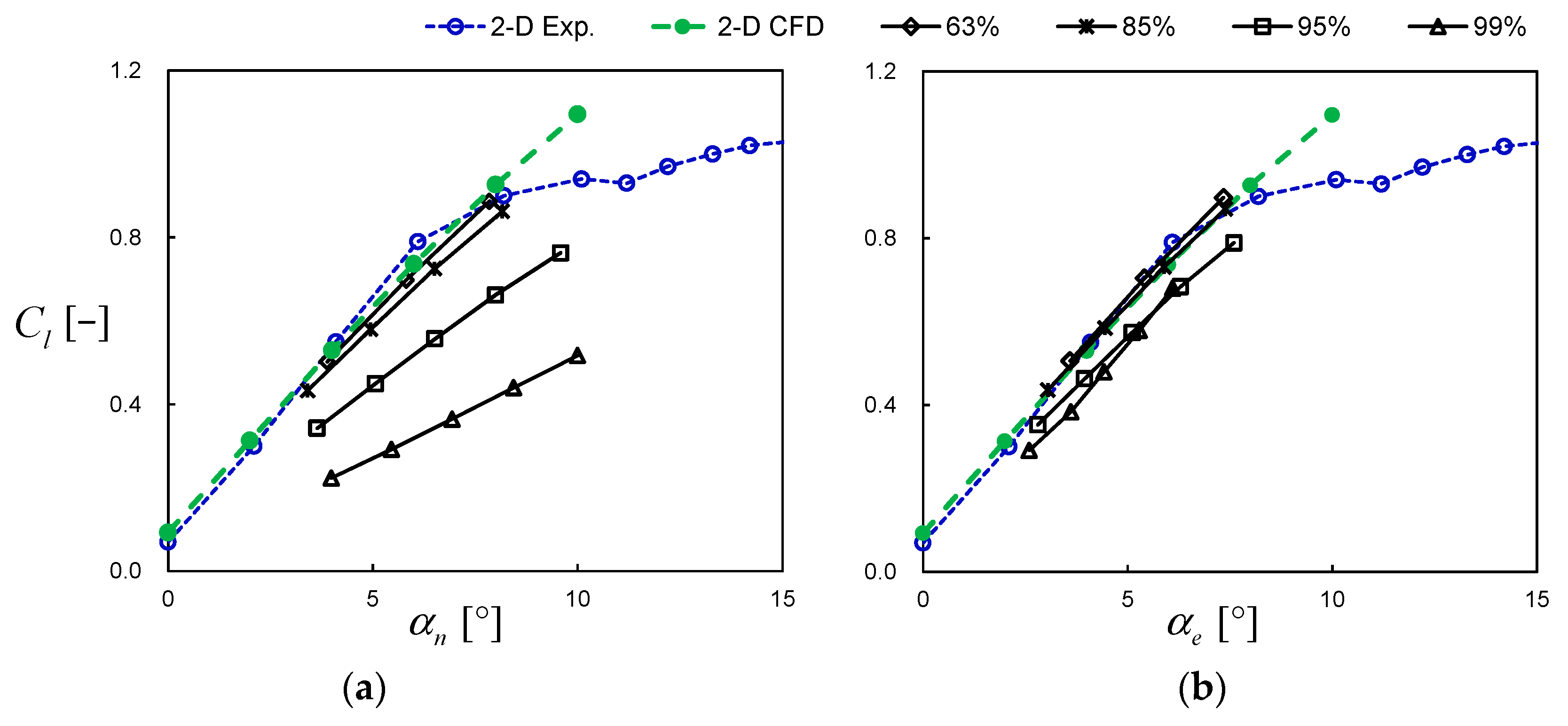
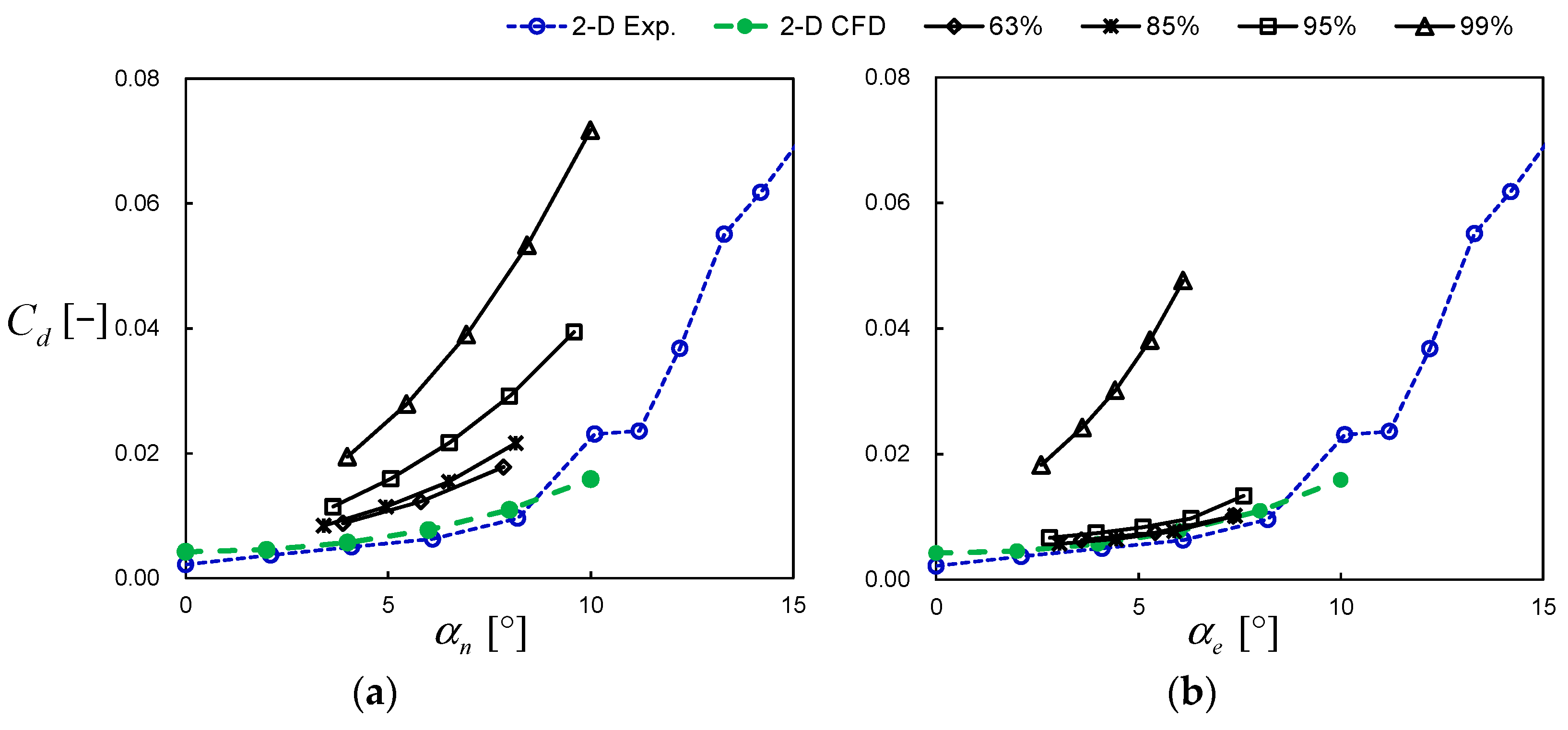
  • The extracted aerodynamic polar of both the mid-board and tip sections are consistent with each other as well as with the 2-D polar, which proves that the so-called 3-D polar is an appearance rather than a substance and the fundamentally aerodynamic difference between a blade section and its 2-D airfoil is caused by the variation of effective AoA. In fact, this conclusion is a basis of the BEM, VWT, or AL/NS method that determines the section forces from the 2-D airfoil data according to the effective AoA.
In addition, the present method provides a potential approach to use the full CFD simulation with blade entities to validate the velocity at the blade axis in BEM, VWT, or AL/NS computations. The present method could also be applicable to experimental results if the velocity of the monitoring points and the pressure distribution of multiple sections are measured. Nevertheless, the method becomes questionable when flow separation occurs, since the Kutta–Joukowski law no longer holds under this situation. In the present study, the determination of AoA is not performed in conditions of high wind speed ( V 10 m/s) at which flow separation occurs on a large area of this stall-regulated rotor, which is a limitation of the present method. Fortunately, for modern commercial wind turbines with pitch control, flow separation rarely happens in the blade tip region where the effective AoA is of great significance. In the future work, the present method can be applied to more wind turbines under axial and yawed conditions for a more comprehensive evaluation.

Author Contributions

Formal analysis, W.Z.; funding acquisition, W.Z. and T.G.W.; investigation, W.Z.; methodology, W.Z. and W.Z.S.; resources, W.J.Z.; supervision, W.Z.S. and T.G.W.; writing—original draft, W.Z.; writing—review and editing, W.Z.S., T.G.W., and W.J.Z.

Funding

This work was funded jointly by the National Natural Science Foundation of China (No. 51506088), the National Basic Research Program of China (“973” Program) under Grant No. 2014CB046200, the Priority Academic Program Development of Jiangsu Higher Education Institutions, and the Key Laboratory of Wind Energy Utilization, Chinese Academy of Sciences (No. KLWEU- 2016-0102).

Acknowledgments

The first author was awarded a scholarship by the China Scholarship Council (CSC) for studying in Department of Wind Energy, Technical University of Denmark (DTU) as a visiting scholar in a period of 1 year from January 2015 to January 2016 when the present study was started. The first author wishes to express his gratitude to CSC and DTU.

Conflicts of Interest

The authors declare no conflict of interest.

Nomenclature

a axial interference factor
Bnumber of blades
cchord length
Cl, Cdlift and drag coefficients
Cn, Ctnormal and tangential force coefficients
e an unit vector
i unit vector in the x direction
j unit vector in the y direction
k unit vector in the z direction
Llift
l k length of a segment
p pressure
p k pressure on the kth segment
p pressure of the undisturbed wind
rradial location of a blade cross-section
Rrotor radius
v local velocity
v ˜ a axial velocity after self-induction subtraction
v ˜ t tangential velocity after self-induction subtraction
v k local velocity on the kth segment
v induced velocity
v v o r t i c e s induced velocity of distributed vortices
v a i r f o i l induced velocity of airfoil entity
V wind speed
αangle of attack
αeeffective angle of attack
αidownwash angle
αnnominal angle of attack
γ k circulation of kth vortex
Γcirculation of concentrated vortex
δ relative error
θlocal pitch angle
ρair density
ψazimuthal angle
ω rotational speed

References

  1. Global Wind Report 2018; Global Wind Energy Council: Brussels, Belgium, April 2019.
  2. Renewables 2019 Global Status Report; REN21: Paris, France, 2019.
  3. Ghanaatian, M.; Lotfifard, S. Control of Flywheel Energy Storage Systems in the Presence of Uncertainties. IEEE Trans. Sustain. Energy 2018, 10, 36–45. [Google Scholar] [CrossRef]
  4. Ghanbari, N.; Shabestari, P.M.; Mehrizi-Sani, A.; Bhattacharya, S. State-Space Modeling and Reachability Analysis for a DC Microgrid. In Proceedings of the 2019 IEEE Applied Power Electronics Conference and Exposition (APEC), Anaheim, CA, USA, 17–21 March 2019; Institute of Electrical and Electronics Engineers (IEEE): Washington, DC, USA, 2019; pp. 2882–2886. [Google Scholar]
  5. Shen, W.Z. Special Issue on Wind Turbine Aerodynamics. Appl. Sci. 2019, 9, 1725. [Google Scholar] [CrossRef]
  6. Bai, C.-J.; Wang, W.-C. Review of computational and experimental approaches to analysis of aerodynamic performance in horizontal-axis wind turbines (HAWTs). Renew. Sustain. Energy Rev. 2016, 63, 506–519. [Google Scholar] [CrossRef]
  7. Snel, H. Review of Aerodynamics for Wind Turbines. Wind Energy 2003, 6, 203–211. [Google Scholar] [CrossRef]
  8. Hansen, M.O.L. The classical blade element momentum method. In Aerodynamics of Wind Turbines, 3rd ed.; Routledge: Abingdon, UK, 2015; pp. 38–53. [Google Scholar]
  9. Sørensen, J.N. General Momentum Theory for Horizontal Axis Wind Turbines; Springer Science and Business Media LLC: New York, NY, USA, 2016; Volume 4, pp. 123–132. [Google Scholar]
  10. Rehman, S.; Alam, M.M.; Alhems, L.M.; Rafique, M.M. Horizontal Axis Wind Turbine Blade Design Methodologies for Efficiency Enhancement—A Review. Energies 2018, 11, 506. [Google Scholar] [CrossRef]
  11. Wang, T.G. Unsteady Aerodynamic Modeling of Horizontal Axis Wind Turbine Performance. Ph.D. Thesis, University of Glasgow, Glasgow, UK, 1999. [Google Scholar]
  12. Shaler, K.; Kecskemety, K.M.; McNamara, J.J. Benchmarking of a Free Vortex Wake Model for Prediction of Wake Interactions. Renew. Energy 2019, 136, 607–620. [Google Scholar] [CrossRef]
  13. Zhong, W.; Tang, H.; Wang, T.; Zhu, C. Accurate RANS Simulation of Wind Turbine Stall by Turbulence Coefficient Calibration. Appl. Sci. 2018, 8, 1444. [Google Scholar] [CrossRef]
  14. Sumner, J.; Watters, C.S.; Masson, C. CFD in Wind Energy: The Virtual, Multiscale Wind Tunnel. Energies 2010, 3, 989–1013. [Google Scholar] [CrossRef] [Green Version]
  15. Van Kuik, G.A.M.; Sørensen, J.N.; Okulov, V.L. Rotor theories by professor Joukowsky: Momentum theories. Prog. Aerosp. Sci. 2015, 73, 1–18. [Google Scholar] [CrossRef]
  16. Shen, W.Z.; Mikkelsen, R.; Sørensen, J.N.; Bak, C. Tip loss corrections for wind turbine computations. Wind Energy 2005, 8, 457–475. [Google Scholar] [CrossRef]
  17. Zhong, W.; Shen, W.; Wang, T.; Li, Y. A tip loss correction model for wind turbine aerodynamic performance prediction. Renew. Energy 2020, 147, 223–238, in press. [Google Scholar] [CrossRef]
  18. Zhu, C.; Wang, T.; Zhong, W. Combined Effect of Rotational Augmentation and Dynamic Stall on a Horizontal Axis Wind Turbine. Energies 2019, 12, 1434. [Google Scholar] [CrossRef]
  19. Snel, H.; Houwink, R.; Bosschers, J. Sectional Prediction of Lift Coefficients on Rotating Wind Turbine Blades in Stall; ECN-C-93-052; ECN: Petten, The Netherlands, 1993. [Google Scholar]
  20. Buining, A.; van Bussel, G.J.W.; Corten, C.P.; Timmer, W.A. Pressure Distributions from a Wind Turbine Blade: Field Measurements Compared to 2-Dimensional Wind Tunnel Data; DUT-IVW-93065R; Delft University of Technology: Delft, The Netherlands, 1993. [Google Scholar]
  21. Laino, D.; Hansen, A.; Minnema, J. Validation of the AeroDyn subroutines using NREL unsteady aerodynamics experiment data. Wind Energy 2002, 5, 227–244. [Google Scholar] [CrossRef]
  22. Lindenburg, C. Investigation into Rotor Blade Aerodynamics—Analysis of the Stationary Measurements on the UAE Phase-VI Rotor in the NASA-Ames Wind Tunnel; ECN: Petten, The Netherlands, 2003. [Google Scholar]
  23. Bak, C.; Johansen, J.; Andersen, P.B. Three-dimensional corrections of airfoil characteristics based on pressure distributions. In Proceedings of the European Wind Energy Conference (EWEC 06), Athens, Greece, 27 February–2 March 2006. BL3.356. [Google Scholar]
  24. Sant, T.; Van Kuik, G.; Van Bussel, G.J.W. Estimating the angle of attack from blade pressure measurements on the NREL Phase VI rotor using a free wake vortex model: Axial conditions. Wind Energy 2006, 9, 549–577. [Google Scholar] [CrossRef]
  25. Sant, T.; van Kuik, G.; van Bussel, G.J.W. Estimating the angle of attack from blade pressure measurements on the NREL phase VI rotor using a free wake vortex model: Yawed conditions. Wind Energy 2009, 12, 1–32. [Google Scholar] [CrossRef]
  26. Bretton, S.-P.; Sibuet Watters, C.; Masson, C. Study of the Angle of Attack on a Wind Turbine Blade Using a Vortex Wake Lifting Line Method; The Science of Making Torque from Wind: Crete, Greece, 2010. [Google Scholar]
  27. Hansen, M.O.; Sørensen, N.N.; Michelsen, J.N. Extraction of lift, drag and angle of attack from computed 3-D viscous flow around a rotating blade. In Proceedings of the EWEC, Dublin, Ireland, 6–9 October 1997; pp. 499–501. [Google Scholar]
  28. Johansen, J.; Sørensen, N. Aerofoil characteristics from 3D rotor CFD simulations. Wind Energy 2004, 7, 283–294. [Google Scholar] [CrossRef]
  29. Jost, E.; Klein, L.; Leipprand, H.; Lutz, T.; Krämer, E. Extracting the angle of attack on rotor blades from CFD simulations. Wind Energy 2018, 21, 807–822. [Google Scholar] [CrossRef]
  30. Rahimi, H.; Hartvelt, M.; Peinke, J.; Schepers, J. Investigation of the current yaw engineering models for simulation of wind turbines in BEM and comparison with CFD and experiment. J. Phys. Conf. Ser. 2016, 753, 022016. [Google Scholar] [CrossRef] [Green Version]
  31. Herráez, I.; Daniele, E.; Schepers, J.G. Extraction of the wake induction and angle of attack on rotating wind turbine blades from PIV and CFD results. Wind Energy Sci. 2018, 3, 1–9. [Google Scholar] [CrossRef] [Green Version]
  32. Shen, W.Z.; Hansen, M.O.L.; Sørensen, J.N. Determination of angle of attack (AOA) for rotating blades. In Proceedings of the Euromech Colloquium—Wind Energy; Springer: Berlin/Heidelberg, Germany, 2006; pp. 205–209. [Google Scholar]
  33. Shen, W.Z.; Hansen, M.O.L.; Sørensen, J.N.; Sørensen, J.N. Determination of the angle of attack on rotor blades. Wind Energy 2009, 12, 91–98. [Google Scholar] [CrossRef]
  34. Yang, H.; Shen, W.Z.; Sørensen, J.N.; Zhu, W.J. Extraction of airfoil data using PIV and pressure measurements. Wind Energy 2011, 14, 539–556. [Google Scholar] [CrossRef]
  35. Yang, H.; Shen, W.; Sørensen, J.N.; Zhu, W. Investigation of load prediction on the Mexico rotor using the technique of determination of the angle of attack. Chin. J. Mech. Eng. 2012, 25, 506–514. [Google Scholar] [CrossRef]
  36. Schneider, M.S.; Nitzsche, J.; Hennings, H. Accurate load prediction by BEM with airfoil data from 3D RANS simulations. J. Phys. Conf. Ser. 2016, 753, 82016. [Google Scholar] [CrossRef] [Green Version]
  37. Syed Ahmed Kabir, I.F.; Ng, E.Y.K. Insight into stall delay and computation of 3D sectional aerofoil characteristics of NREL phase Ⅵ wind turbine using inverse BEM and improvement in BEM analysis accounting for stall delay effect. Energy 2017, 120, 518–536. [Google Scholar] [CrossRef]
  38. Wimshurst, A.; Willden, R.H.J. Extracting lift and drag polars from blade-resolved computational fluid dynamics for use in actuator line modelling of horizontal axis turbines. Wind Energy 2017, 20, 815–833. [Google Scholar] [CrossRef]
  39. Elgammi, M.; Sant, T. Combining Unsteady Blade Pressure Measurements and a Free-Wake Vortex Model to Investigate the Cycle-to-Cycle Variations in Wind Turbine Aerodynamic Blade Loads in Yaw. Energies 2016, 9, 460. [Google Scholar] [CrossRef]
  40. Wen, B.; Tian, X.; Dong, X.; Peng, Z.; Zhang, W.; Wei, K. A numerical study on the angle of attack to the blade of a horizontal-axis offshore floating wind turbine under static and dynamic yawed conditions. Energy 2019, 168, 1138–1156. [Google Scholar] [CrossRef]
  41. Wu, G.; Zhang, L.; Yang, K. Development and Validation of Aerodynamic Measurement on a Horizontal Axis Wind Turbine in the Field. Appl. Sci. 2019, 9, 482. [Google Scholar] [CrossRef]
  42. Schepers, J.G.; Boorsma, K.; Cho, T.; Gomez-Iradi, S.; Schaffarczyk, P.; Jeromin, A.; Lutz, T.; Meister, K.; Stoevesandt, B.; Schreck, S.; et al. Final Report of IEA Task 29, Mexnext (Phase 1): Analysis of MEXICO Wind Tunnel Measurements; Technical Report ECN-E12-004; Energy Research Centre of the Netherlands (ECN): Amsterdam, The Netherlands, 2012. [Google Scholar]
  43. Guntur, S.; Sørensen, N.N. An evaluation of several methods of determining the local angle of attack on wind turbine blades. J. Phys. Conf. Ser. 2014, 555, 012045. [Google Scholar] [CrossRef] [Green Version]
  44. Rahimi, H.; Schepers, J.; Shen, W.; García, N.R.; Schneider, M.; Micallef, D.; Ferreira, C.S.; Jost, E.; Klein, L.; Herráez, I. Evaluation of different methods for determining the angle of attack on wind turbine blades with CFD results under axial inflow conditions. Renew. Energy 2018, 125, 866–876. [Google Scholar] [CrossRef] [Green Version]
  45. Hand, M.M.; Simms, D.A.; Fingersh, L.J.; Jager, D.W.; Cotrell, J.R.; Schreck, S.; Larwood, S.M. Unsteady Aerodynamics Experiment Phase VI: Wind Tunnel Test Configurations and Available Data Campaigns; NREL/TP-500-29955; National Renewable Energy Laboratory: Golden, CO, USA, 2001. [Google Scholar]
  46. Schlichting, H. Boundary-Layer Theory, 7th ed.; McGraw-Hill Book Company: New York, NY, USA, 1979. [Google Scholar]
  47. Ramsay, R.; Hoffman, M.; Gregorek, G. Effects of Grit Roughness and Pitch Oscillations on the S809 Airfoil; NREL/TP-442-7817; National Renewable Energy Laboratory: Golden, CO, USA, 1995. [Google Scholar]
  48. Sørensen, J.N.; Dag, K.O.; Ramos-Garía, N. A new tip correction based on the decambering approach. J. Phys. Conf. Ser. 2015, 524, 012097. [Google Scholar] [CrossRef]
Figure 1. Different kinds of inductions in the flattened section of a certain radial location: (a) Bent streamlines because of disc-induction; (b) self-induction; (c) downwash because of 3D-induction.
Energies 12 04012 g001
Figure 2. Illustration of the concentrated vortex of an airfoil.
Energies 12 04012 g002
Figure 3. Illustration of the distributed vortices on an airfoil: (a) vortices; (b) viscous flow on a small segment.
Energies 12 04012 g003
Figure 4. Contours of dimensionless-induced velocity: (a) Induced by the airfoil entity, | v a i r f o i l | / V ; (b) induced by the distributed vortices, | v v o r t i c e s | / V (Airfoil S809, α = 6 ° , Reynolds number = 1 × 10 6 ).
Energies 12 04012 g004
Figure 5. Contours of relative error (Airfoil S809, α = 6 ° , Reynolds number = 1 × 10⁶).
Energies 12 04012 g005
Figure 6. Illustration of the vortex at a small face of blade surface: the faces are intentionally enlarged in order to be displayed clearly.
Energies 12 04012 g006
Figure 7. Contours of axial interference factor before self-induction subtraction in the flattened section of r/R = 47%, where ψ denotes the azimuthal angle ( V = 7 m / s , ω = 72 rpm ).
Energies 12 04012 g007
Figure 8. Contours of axial interference factor after self-induction subtraction in the flattened section of r/R = 47% ( V = 7 m / s , ω = 72 rpm ).
Energies 12 04012 g008
Figure 9. Variation of axial interference factor with azimuthal angle in the rotor plane at r/R = 47% ( V = 7 m / s , ω = 72 rpm ).
Energies 12 04012 g009
Figure 10. Contours of axial interference factor after the self-induction subtraction in the flatten section of r/R = 95% ( V = 7 m / s , ω = 72 rpm ).
Energies 12 04012 g010
Figure 11. Contours of axial interference factor after the self-induction subtraction around the blade the dashed black line is a typical contour line ( V = 7 m / s , ω = 72 rpm ).
Energies 12 04012 g011
Figure 12. Values of AoA determined by the local velocity after the self-induction subtraction at various azimuthal locations on the r/R = 95% ring in the rotor plane; the dashed black curves near the blade axis as well as the effective AoA are estimated ( V = 7 m / s , ω = 72 rpm ).
Energies 12 04012 g012
Figure 13. Contours of AoA determined by the local velocity after the self-induction subtraction in the flattened section of r/R = 95%; the solid points P1, P2, P3, P1’, P2’, P3’ are the monitoring points of 3-point AT; the dashed circle are used for Line AT; the star points A and A’ are the monitoring points of the present determination ( V = 7 m / s , ω = 72 rpm ).
Energies 12 04012 g013
Figure 14. Variation of AoA along the blade span: (a) nominal AoA; (b) effective AoA.
Energies 12 04012 g014
Figure 15. Variation of the downwash angle along the blade span: (a) downwash angle; (b) the ratio of downwash angle to nominal AoA.
Energies 12 04012 g015
Figure 16. Lift coefficient extracted through: (a) nominal AoA; (b) effective AoA.
Energies 12 04012 g016
Figure 17. Drag coefficient extracted through: (a) nominal AoA; (b) effective AoA.
Energies 12 04012 g017
Table 1. List of the angle of attack (AoA) determination methods and their corresponding kinds of AoA.
MethodAoAMethodAoA
Inverse BEM [19,20,21,22,23]Effective3-point AT [30]Blended
Inverse VWT [24,25,26]EffectiveSIS1 [32]Nominal
AAT [27,28]NominalSIS2 [33]Nominal
Line AT [29]Blended

