Article

An Electro-Pneumatic Force Tracking System using Fuzzy Logic Based Volume Flow Control

1
Jiangsu Province Key Laboratory of Aerospace Power System, College of Energy and Power Engineering, Nanjing University of Aeronautics and Astronautics, Nanjing 210016, China
2
Centre for Propulsion Engineering, School of Aerospace, Transport, and Manufacturing, Cranfield University, Central Bedfordshire MK43 0AL, UK
*
Author to whom correspondence should be addressed.
Energies 2019, 12(20), 4011; https://doi.org/10.3390/en12204011
Submission received: 25 September 2019 / Revised: 17 October 2019 / Accepted: 19 October 2019 / Published: 22 October 2019

Abstract

:
In this paper, a fuzzy logic based volume flow control method is proposed to precisely control the force of a pneumatic actuator in an electro-pneumatic system including four on-off valves. The volume flow feature, which is the relationship between the duty cycle of the pulse width modulation (PWM) period, pressure difference, and volume flow of an on-off valve, is based on the experimental data measured by a high-precision volume flow meter. Through experimental data analysis, the maximum and minimum duty cycles are acquired. A new volume flow control method is introduced for the pneumatic system. In this method, the raw measured data are innovatively processed by a segmented, polynomial fitting method, and a newly designed procedure for calculating the duty cycle is adopted. This procedure makes it possible to combine the original data with fuzzy logic control (FLC). Additionally, the method allows us to accurately control the minimum and maximum opening pulse width of the valve. Several experiments are performed based on the experimental data, instead of the traditional theoretical models. Only 0.141 N (1.41%) overshoot and 0.03 N (0.03%) steady-state error are observed in the step response experiment, and 0.123 N average error is found while tracking the sine wave reference.

Graphical Abstract

1. Introduction

In modern society, especially in industry, pneumatic control systems which use compressed gas to transfer and control energy have been widely used to drive automated machinery such as the metro door switch, production line operations, robotic arms, and in the aerospace industry. Compared to hydraulic control systems, it has a number of irreplaceable advantages: high efficiency, durability and reliability, simple structure, clean energy, easy maintenance, and low price. Pneumatic control valves have developed rapidly over the past twenty years. In the early research, proportional or servo valves are mentioned mostly for their continuous and linear output characteristics [1,2]. However, the defects of this kind of valve are equally distinct: a slow response speed, high expense, and difficult maintenance. An alternative is solenoid on-off valves, due to their low price and easy maintenance. Traditional on-off valves do not have the characteristic of fast response, and the opening times for those valves are usually more than 5 ms [3,4]. Over the past ten years, research on increasing the switching speed of the on-off valve using digital acceleration technology [5,6] has shown increasing possibilities for using the on-off valves instead of the servo valves.
There are two approaches which are often mentioned in traditional pneumatic control studies: pulse width modulation (PWM) and theoretical modeling. The conventional PWM technique is generally used for on-off valves [7,8]. For on-off valves, especially the fast response on-off valves using digital acceleration technology, the PWM technique is a very effective way to make the volume flow close to linearity [9,10]. However, for the PWM method and the high-speed on-off valve, the dead zone problem has always existed, which severely restricts the development of the high-speed on-off valve [11,12]. Many improved methods such as modified differential PWM (MD-PWM) [13], the five and seven modes switching method [14], and phase-change PWM [15] are proposed to deal with the dead zone problem. These methods do have a particular effect on the dead zone compensation, but they are not perfect.
Theoretical modeling is the basis of pneumatic control research. Many early works present the modeling of pneumatic actuators [16,17]. Similarly, there are also articles which study the modeling of pneumatic valves. Taghizadeh M. et al. [5] described the complete nonlinear dynamic modeling method for a 3/2 solenoid on-off valve, and some identifications are also given. Pohl J. et al. [18] present a model of the 2/2 solenoid valve, and the model parameters are well tuned. However, the complete valve models are often ignored in control-oriented researches [19,20]. This type of research usually uses the traditional theoretical model for the mass or volume flow rate through an orifice to represent the whole valve model. It is very inaccurate to use the simplified model and may cause problems in the following experiments. To solve this problem, Pipan M. and Herakovič N. [21,22] proposed a measuring method to find the correlation between the PWM frequency, the PWM duty cycle, and the volume flow of a PWM-driven valve. This method is a good replacement for traditional modeling. It is especially suitable to be used in the controller design. Based on these works, an improved volume flow control method is introduced in this paper. A segmented, polynomial fitting method and a newly designed method for calculating the duty cycle are adopted.
Several advanced control algorithms [23,24,25] including the proportional–integral–derivative (PID) control and fuzzy logic control (FLC) have been widely studied over the past decade. Many advanced PID controllers such as the nonlinear PID (N-PID) controller and multi-rate nonlinear PID (MN-PID) controller have been proposed to solve the strong nonlinear problem of the pneumatic control systems [26,27], as fuzzy logic control can be easily combined with PWM or other controllers. Shih M.C. and Hwang C.G. [28] proposed a fuzzy PWM method in 1997 to control a pneumatic robot cylinder with solenoid valves. Salim S. et al. [27] proposed a unique method to combine the fuzzy nonlinear gain with the N-PID controller. These methods showed excellent performance when tracking the referenced position signals. This paper is focused on an improved volume flow control method with fuzzy logic control. The fuzzy logic controller is adjusted for the force tracking system, which is a highly asymmetrical and nonlinear system. Additionally, a field programmable gate array (FPGA) platform is utilized as the primary control platform for real-time control in this paper.
In this paper, an improved volume flow control method with fuzzy logic control is applied in a force tracking system. The volume flow data are firstly acquired by several high-precision instruments. In the original volume flow control method from Pipan M. and Herakovič N. [21,22], the method of raw volume flow data with simple interpolation was used to control the valve. Based on their research, we manage to apply the segmented, polynomial fitting method to process the data. At the same time, we develop a new method for calculating the duty cycle which is completely different from the original method. By utilizing this method, the raw data of the volume flow can be combined with the classic fuzzy logic controller. Due to strong nonlinearities of the force tracking system, fuzzy rules are completely asymmetrical, and every rule is designed based on the real experimental results. The force tracking system includes a double-acting double-rod-end cylinder and four fast response on-off valves. Following the introduction section, the article is organized as follows: the testing method, experimental setup of measuring the volume flow, and testing results for the volume flow feature of the solenoid on-off valve are introduced in Section 2. In Section 3, controller designs for the force tracking system including the improved volume flow control method, fuzzy logic controller, and mode selector are introduced. The complete experimental setups are presented in Section 4. In Section 5, experimental results are shown as well as the corresponding discussions. Finally, the conclusion of the work is presented in Section 6.

2. Volume Flow Feature of the Solenoid On-Off Valve
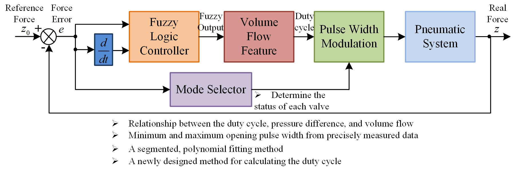
According to the ISO 6358 standard [29], the traditional equation for the volume change rate of the air flow through the orifice of an on-off valve is described as:
d V ( P i n , P o u t ) d t = V ˙ ( P i n , P o u t ) = { P i n C d T 0 T i n , P c P c r P i n C d T 0 T i n 1 ( P c P c r 1 P c r ) 2 , P c > P c r
where V is the volume flow, P i n is the absolute input pressure of the valve, P o u t is the absolute output pressure of the valve, C d is the valve discharge coefficient, T 0 is the stagnation temperature, T i n is the inlet air temperature of the valve, P c = P o u t / P i n is the specific pressure ratio, and P c r = 0.38 is the critical pressure ratio. Equation (1) describes two nonlinear conditions. In the first condition, when the pressure ratio P c is no greater than the critical pressure ratio, the volume change rate of the air flow is linear to the absolute input pressure of the valve. This condition is called sonic (choked) flow. However, when the pressure ratio is bigger than the critical pressure ratio, the air flow dynamics become nonlinear. It depends on both the input and output pressure, and this condition is called subsonic (unchoked) flow. This equation and another equation which describes the mass change rate of the air flow through the orifice of an on-off valve [30] are two classical models to describe the volume or mass change rate of the air flow when the valve orifice is fully open. Whereas in the real control process, the on-off valve needs to be open or closed constantly. In the opening and closing process of the valve, the opening degree of the valve orifice cannot be completely determined. Another critical problem that needs to be taken care of is that the classical model does not show how the volume flow changes when the pulse width for controlling the on-off valve is extremely small or large. We use the real experimental data which are collected from experiments instead of building valve models to solve these problems. This method of acquiring data is originally proposed by Pipan M. and Herakovič N. [21], and their work proves the feasibility of the method. We make some improvements to this method and test it in a different frequency range. The details and results of the method are shown as follows.

2.1. Testing Method

Traditionally, the PWM method is applied to control the on-off valve. The PWM control ‘period’, T t , represents one complete control period for the valve, and the PWM frequency, f p , is defined as:
f p = 1 T t
In one PWM period, the pulse width, t p w , represents the effect control time, so it usually uses ms as its unit. Another description ‘duty cycle’, t p , which uses % as its unit represents the percentage of the pulse width in a PWM period. As the on-off valve used in the final experiments is FESTO model MHJ10-S-0, 35-QS-4-MF which has only 0.9 ms opening time and 0.4 ms closing time, the total switching time for this valve is less than 1.5 ms for one PWM period. So we initially set the possible PWM frequency as 50 Hz, 100 Hz, and 150 Hz. Additionally, the valve discharge coefficient, C d , is 4 × 10⁻⁹ m3/(s·Pa) for this kind of valve.
To successfully acquire the precise data of volume flow, a digital volume flow meter SENSIRION model SFM4200 is applied in this research. The volume flow rate of the air is precisely measured by a thermal sensor element with extremely fast update time and high accuracy. The accuracy of this sensor is 2.5% of the measured value when the value is lower than 80 L/min and 5% of measured value when the value is higher than 80 L/min and the response time is 0.5 ms. The airflow generated by the valve under PWM control fluctuates significantly at the beginning, and it is appropriate to measure the average volume flow after several seconds. We take three seconds to measure and record the average value.
The procedure to measure the volume flow is shown in Figure 1a. The first step, set the PWM frequency, f p , to 50 Hz. As mentioned above, 50 Hz, 100 Hz, and 150 Hz are the frequencies that should be tested. For the second step, we set the pressure difference, Δ P , to 0.01 MPa. We use a pressure regulating valve to precisely adjust the inlet pressure of the valve. As the pressure of the atmosphere, P a t m = 0.1   MPa , the inlet pressure is set to 0.11 MPa. Other pressure differences in this test are 0.03 MPa, 0.05 MPa, 0.07 MPa, 0.1 MPa, 0.15 MPa, 0.2 MPa, and 0.3 MPa. In the third step, we increase the duty cycle, t p , from 0% in 0.1% steps to find the minimum duty cycle, t p m i n , of this pressure difference. Below the minimum duty cycle, there is no air flow through the valve. Steps of 0.1% of the duty cycle are also used to detect the maximum duty cycle, t p m a x . This was chosen to guarantee the accuracy of the entire test. For the fourth step, after finding the minimum duty cycle, we increase t p from 0% to 10% with 1% steps. Following that, in the fifth step, we increase t p from 10% to 100% with 10% steps. At the sixth step, we find the maximum duty cycle, t p m a x , with 0.1% steps. Above the maximum duty cycle, the air flow is nearly invariant. Finally, in the seventh step, we change the pressure difference and go to the third step. After changing the frequency, we repeat the steps from 2 to 7. Figure 1b is the programming interface, and Figure 1c is the main program designed in National Instruments (NI) LabVIEW Pro 11.0.

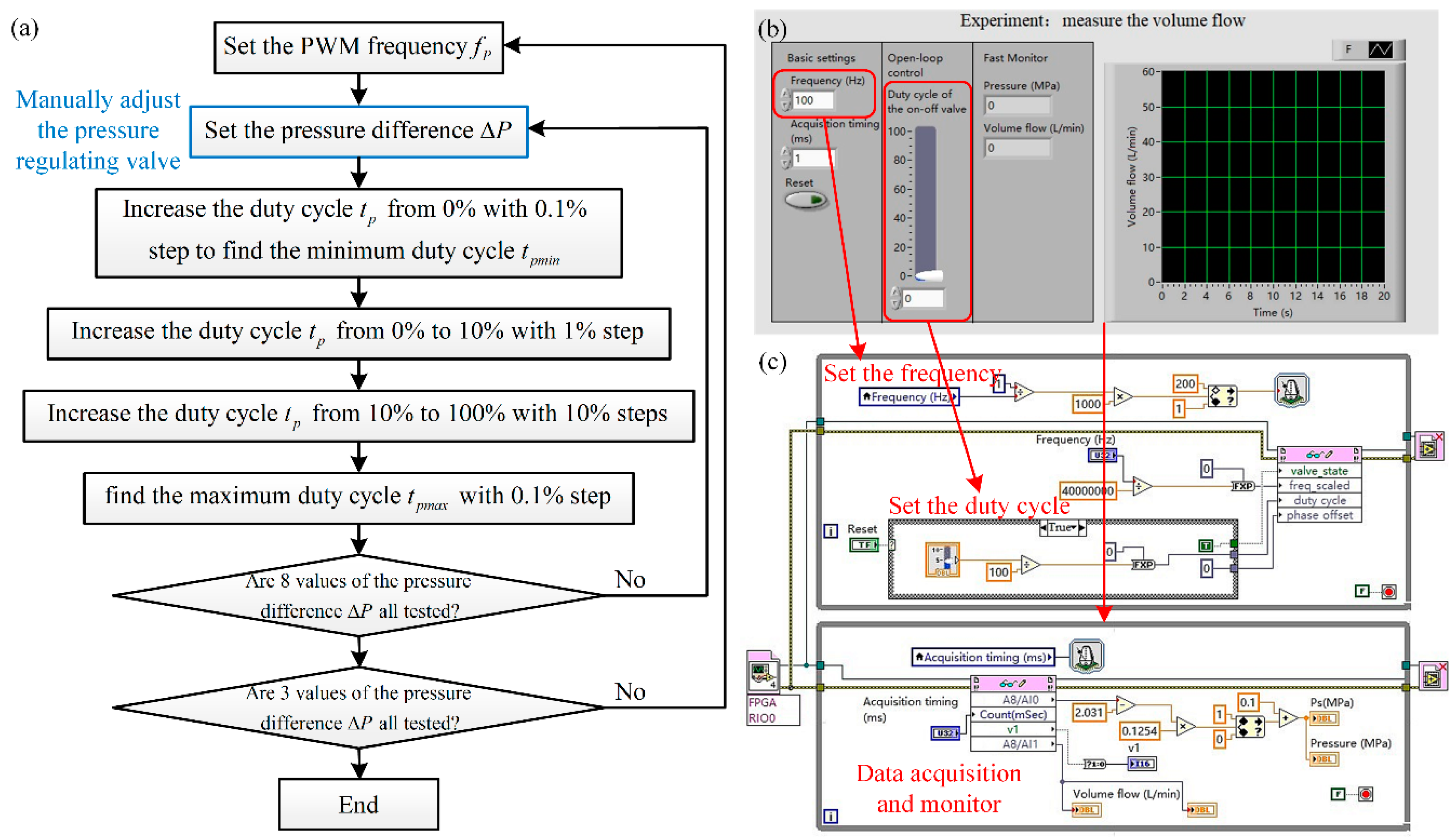
2.2. Experimental Setup of Measuring the Volume Flow

The experimental setup of measuring the volume flow is shown in Figure 2. In the pneumatic setup, the compressed air comes from an air compressor (DENAIR model DVA-11A), a compressed air tank, a refrigerated air dryer, and a filter, regulator, and lubricator (FRL) element. DENAIR model DVA-11A is a standard variable speed drive (VSD) air compressor whose maximum working pressure is 0.85 MPa. It has an ultra-low temperature rise design, and can still operate efficiently even when the frequency is reduced by 50%. The control system can also benefit from the feature that the pressure fluctuation is under 0.1 bar. The FRL element is SMC model AC5000-10D. Its pressure adjusting range is from 0.05 MPa to 0.85 MPa. The FRL element is used to regulate the air supply, clean and filter the water in the compressed air, and extend the working life of the system. The pressure of the compressed air is adjusted by a pressure regulating valve (SMC model AW40-04BG). Its pressure adjusting range is from 0.05 MPa to 0.85 MPa. Since the maximum pressure used in this study is 0.4 MPa, the adjusting range of this pressure regulating valve is sufficient. A silicon-diffused pressure sensor (MEACON model MIK-P300) is used to monitor the pressure. The measurement resolution is up to 0.002 MPa. The fast response valve (FESTO model MHJ10-S-0, 35-QS-4-MF) is connected to a volume flow meter (SENSIRION model SFM4200) after the pressure regulating valve. This valve with inner speed-up control has a response time lower than 0.9 ms, both in the opening and in the closing, with a maximum operating frequency of 1000 Hz. This fast switching feature can effectively improve the system control accuracy. In the volume flow meter, the volume flow rate of the air is precisely measured by a thermal sensor element with an extremely fast update time and high accuracy. By using the most advanced on-off valve and volume flow meter, the accuracy of data acquisition is guaranteed.
In the electrical control part, a compact real-time controller NI model CompactRIO-9074 (cRIO-9074) with a reconfigurable FPGA module is connected to an Intel Core i5 laptop by Ethernet communication. The controller has eight slots for the control cards, 400 MHz Central Processing Unit (CPU), 128 MB RAM (Random Access Memory), 256 MB disk, and a 2 million gate FPGA. It is suitable for industrial control applications and data acquisition. As it has a reconfigurable FPGA module, we choose this controller to real-time control the valves. Two digital input/output (I/O) control cards are installed on cRIO-9074. The digital signal output card (NI model NI-9401) is used to control the on-off valve, and the analog-input differential card (NI model NI-9205) is used for acquiring analog signals from sensors. NI-9401 is a C-series digital output card with 5 V transistor-transistor logic (TTL), 100 ns, and eight channels. NI-9205 is a C-series analog-input differential card with ±10 V, 16-bit, and 32 channels. A circuit including sensor, power, and valve driving is designed to connect the electrical controller and the pneumatic elements.

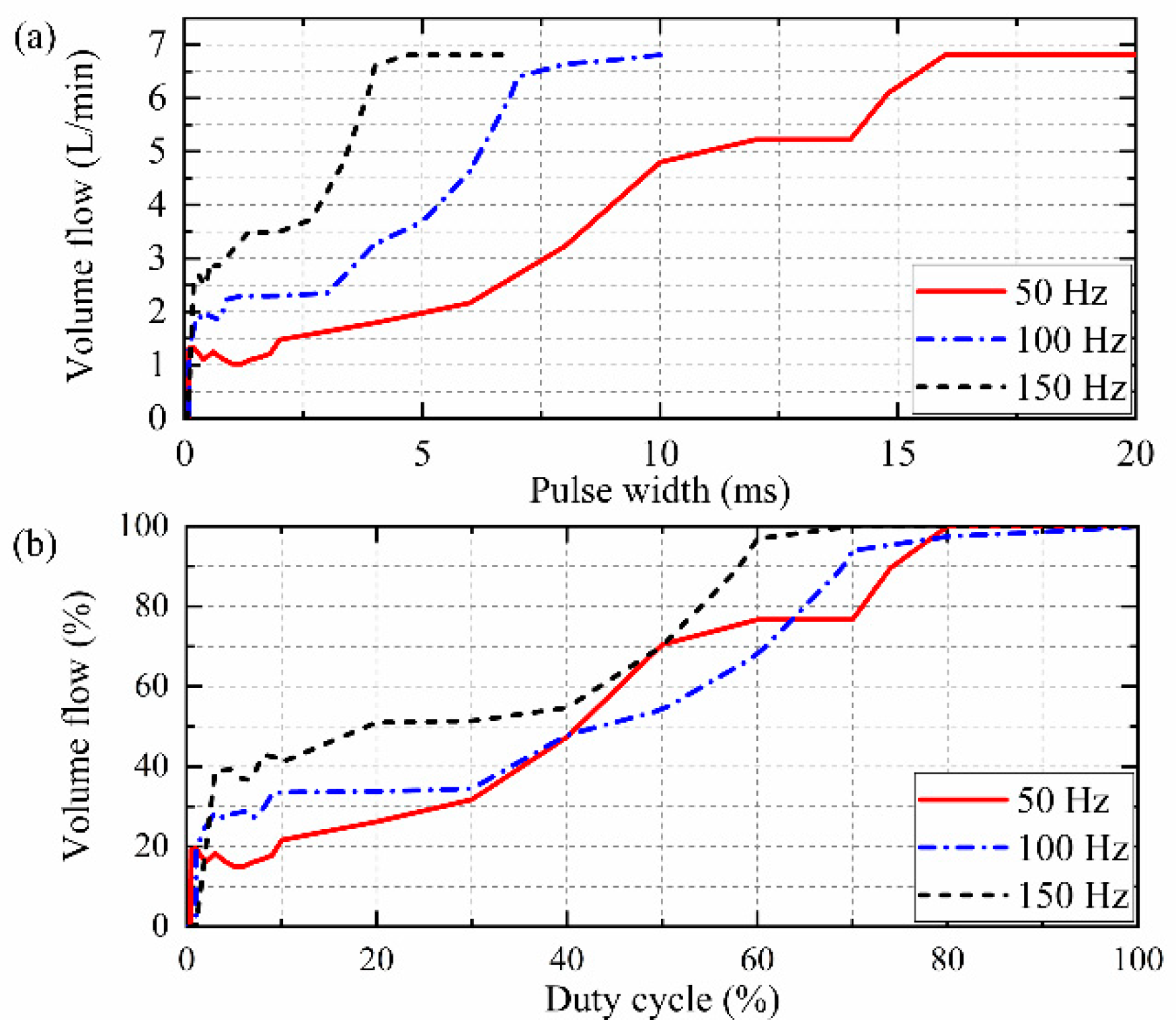
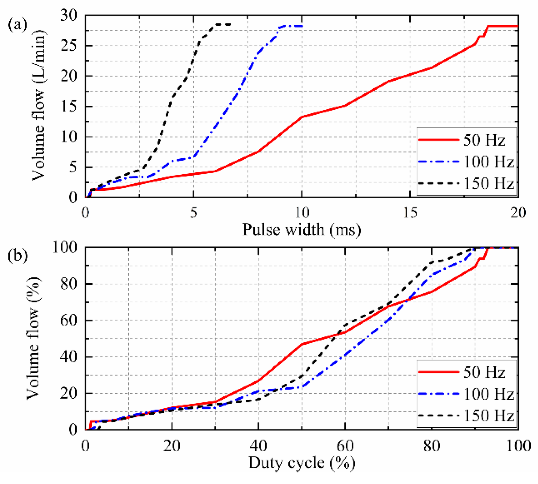
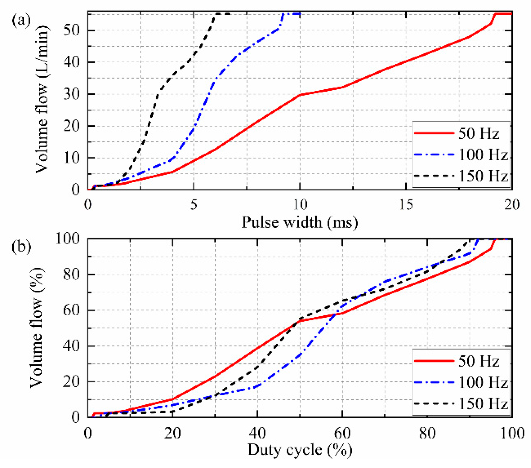
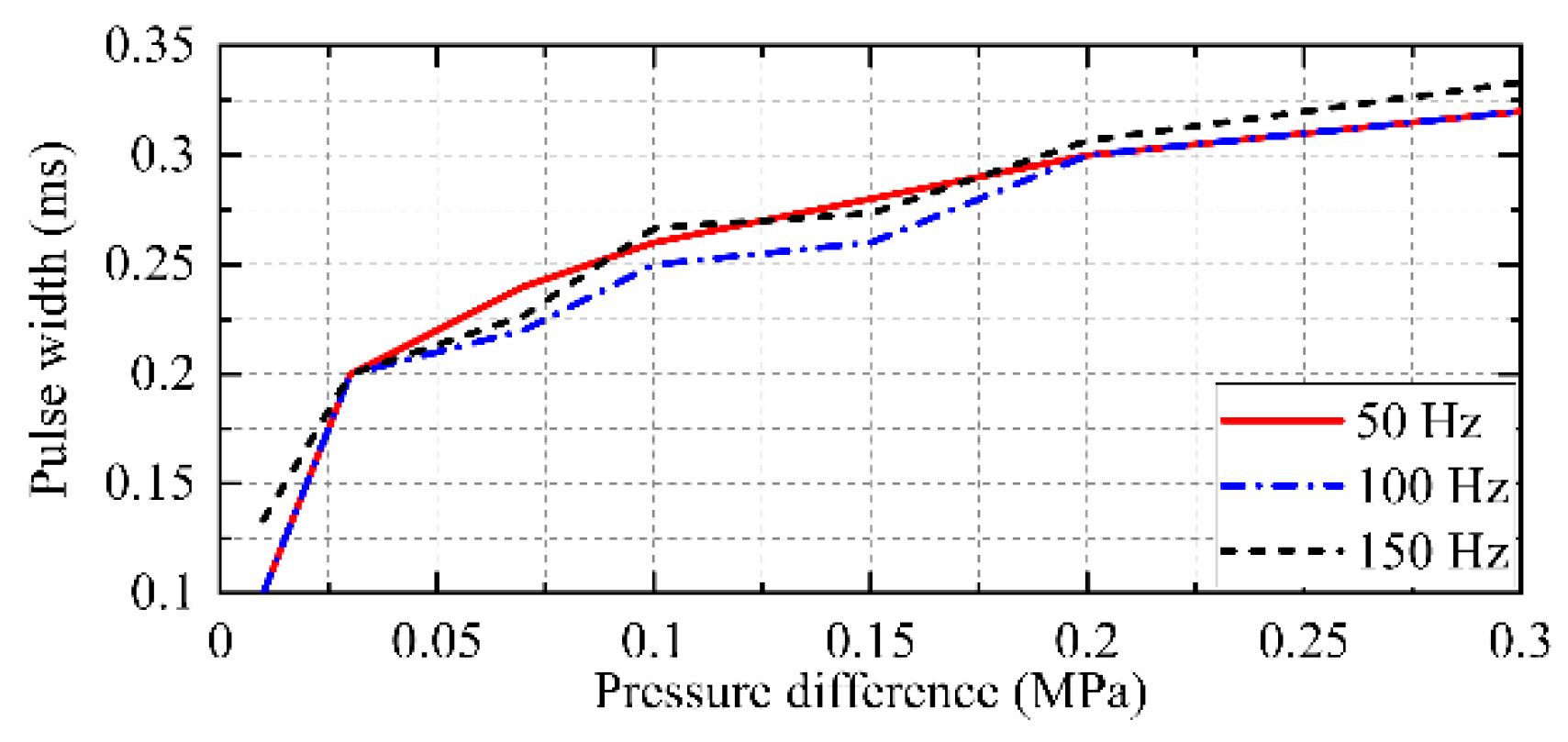
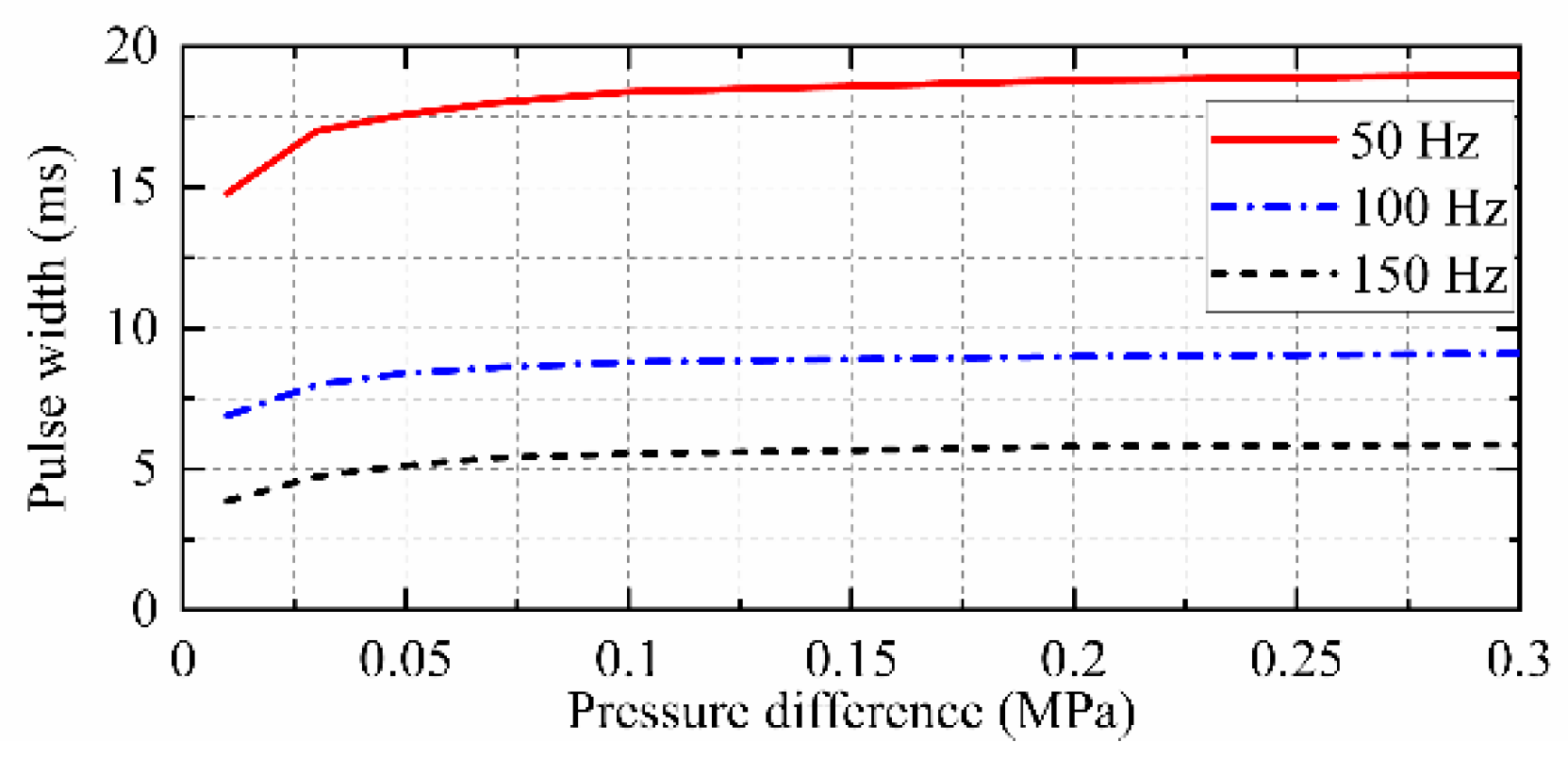
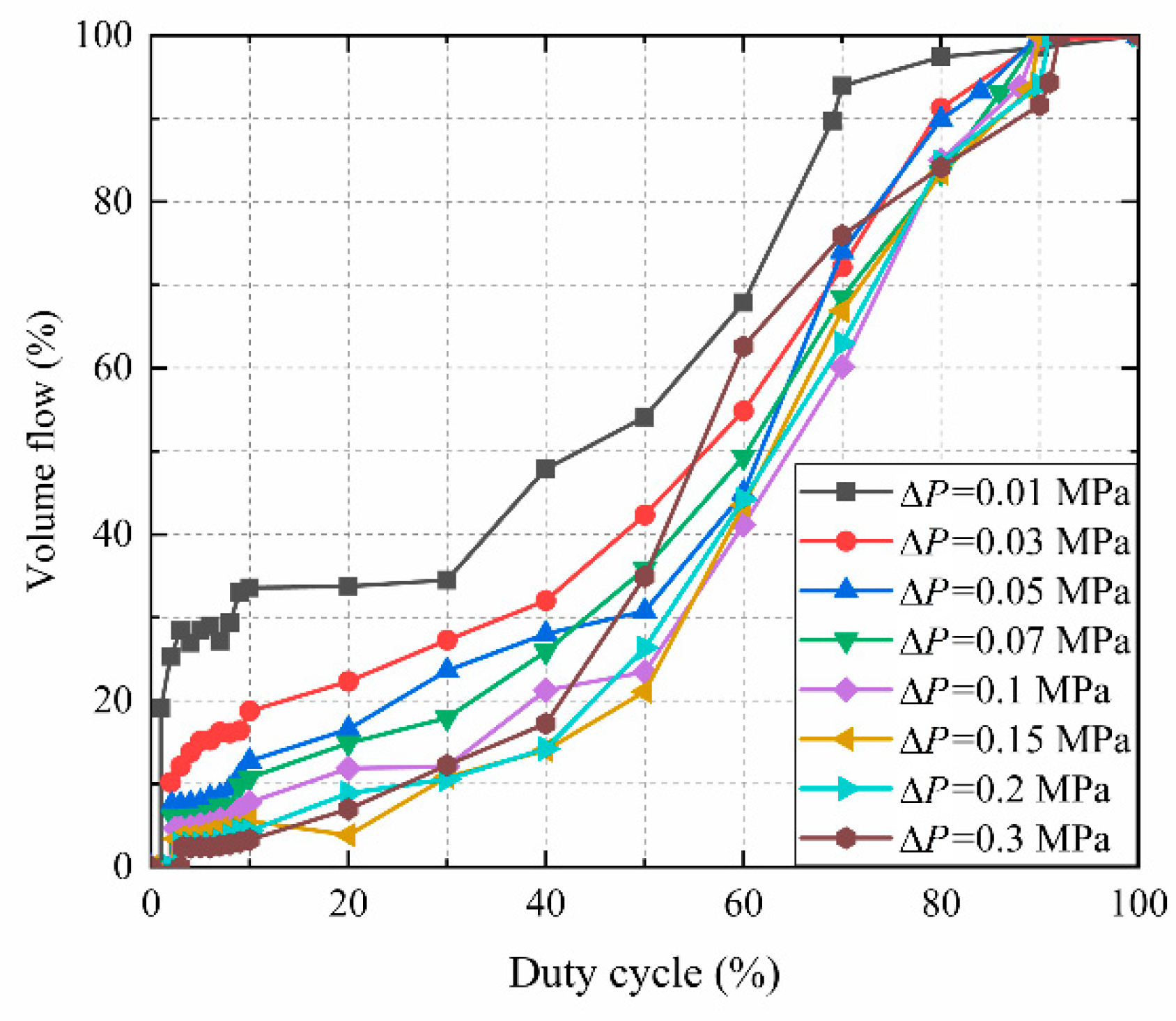
2.3. Testing Results

All the experimental results are acquired and filtered in the cRIO-9074. Several typical results are shown in Figure 3, Figure 4 and Figure 5. We also convert the unit of these results to percentage for a better analysis and use in the following control algorithms. In Figure 3, the pressure difference is 0.01 MPa, which is the lowest pressure difference in our tests. The volume flow rises vertically in the beginning and then increases nonlinearly to a certain value. This vertical raise results from the initial opening of the valve. The maximum pulse width is quite hard to detect as the volume flow keeps increasing all the time under several frequencies. In the following tests, we find that in the control process, above 95% of the biggest volume flow is barely used. So we define the pulse width which generates 95% of the largest volume flow as the maximum pulse width. The maximum pulse width is 14.8 ms (74%) for 50 Hz, 6.9 ms (69%) for 100 Hz, and 3.87 ms (58%) for 150 Hz. In Figure 3b, the results from 50 Hz are much more nonlinear than the results from 100 Hz and 150 Hz.
When the pressure difference is increased to 0.1 MPa, the volume flow results become more linear than the results from a lower pressure difference. In the normalized results, the results for three frequencies are all smooth enough and easy to be fitted. The maximum pulse width is 18.4 ms (92%) for 50 Hz, 8.8 ms (88%) for 100 Hz, and 5.53 ms (83%) for 150 Hz.
Under the biggest pressure difference 0.3 MPa, the relationship between volume flow and pulse width is very close to linearity. The maximum pulse width is 19 ms (95%) for 50 Hz, 9.1 ms (91%) for 100 Hz, and 5.87 ms (88%) for 150 Hz.
It is of great importance to record the minimum pulse width precisely as the pulse width below the minimum value may cause noneffective actions for the valve. In the measuring process, the volume flow value will turn to a small value from 0 when the pulse width is increased from 0% with 0.1% steps of the duty cycle. The relationship between the minimum pulse width and the pressure difference is shown in Figure 6. The pulse width rises from 0.1 ms to 0.33 ms with the increase of pressure difference. Under three different frequencies, the trends of the three curves are very similar, and the difference is quite small.
Similar to the minimum pulse width, the results of the maximum pulse width of three different PWM frequencies under different pressure differences are shown in Figure 7. As the PWM period varies in different frequencies, the three curves do not overlap. However, they still show the same trends. For 50 Hz, the pulse width rises from 14.8 ms to 19 ms, with a fast ascent at the first and remaining unchanged in the following. The pulse width rises from 6.9 ms to 9.1 ms for 100 Hz and from 3.87 ms to 5.87 ms for 150 Hz.
We choose to use 100 Hz as the major control frequency for two reasons: Firstly, the test results of 100 Hz and 150 Hz are both compatible with curve fitting. The data for 50 Hz are extremely nonlinear and not compatible with curve fitting. Secondly, using 100 Hz instead of 150 Hz can also reduce the switching times of the on-off valve. With less valve switching, it can effectively reduce gas fluctuations. The PWM period for 100 Hz is 10 ms. The normalized volume flow results in eight different pressure differences under 100 Hz as shown in Figure 8.
In this section, four conclusions for the volume flow feature of the solenoid on-off valve are achieved by analyzing the experimental results. Firstly, a vertical boost of the volume flow is observed when the pulse width is quite small, especially when the pressure difference is extremely low. Under the extremely low pressure difference, due to the electromagnetic force controlling the movement of the spool, the volume flow is greatly changed. Secondly, as the pressure difference rises, this vertical rise no longer occurs, and the relationship between volume flow and pulse width converges to linearity. Thirdly, the minimum pulse width rises from 0.1 ms to 0.33 ms with the increase of pressure difference. This is due to the stronger pressure force initially influencing the valve spool, and it takes some time for the electromagnetic force to be larger than the pressure force. Under three different frequencies, the three curves are very similar. It means that the minimum pulse width has nothing to do with the frequency. Although the curves of the maximum pulse width under the three different frequencies do not overlap, they still retain the same trends. Finally, 50 Hz is abandoned for its strong nonlinearity under low pressure differences. 100 Hz is chosen instead of 150 Hz to reduce the switching times of the valve.

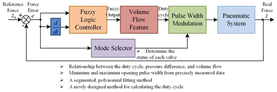
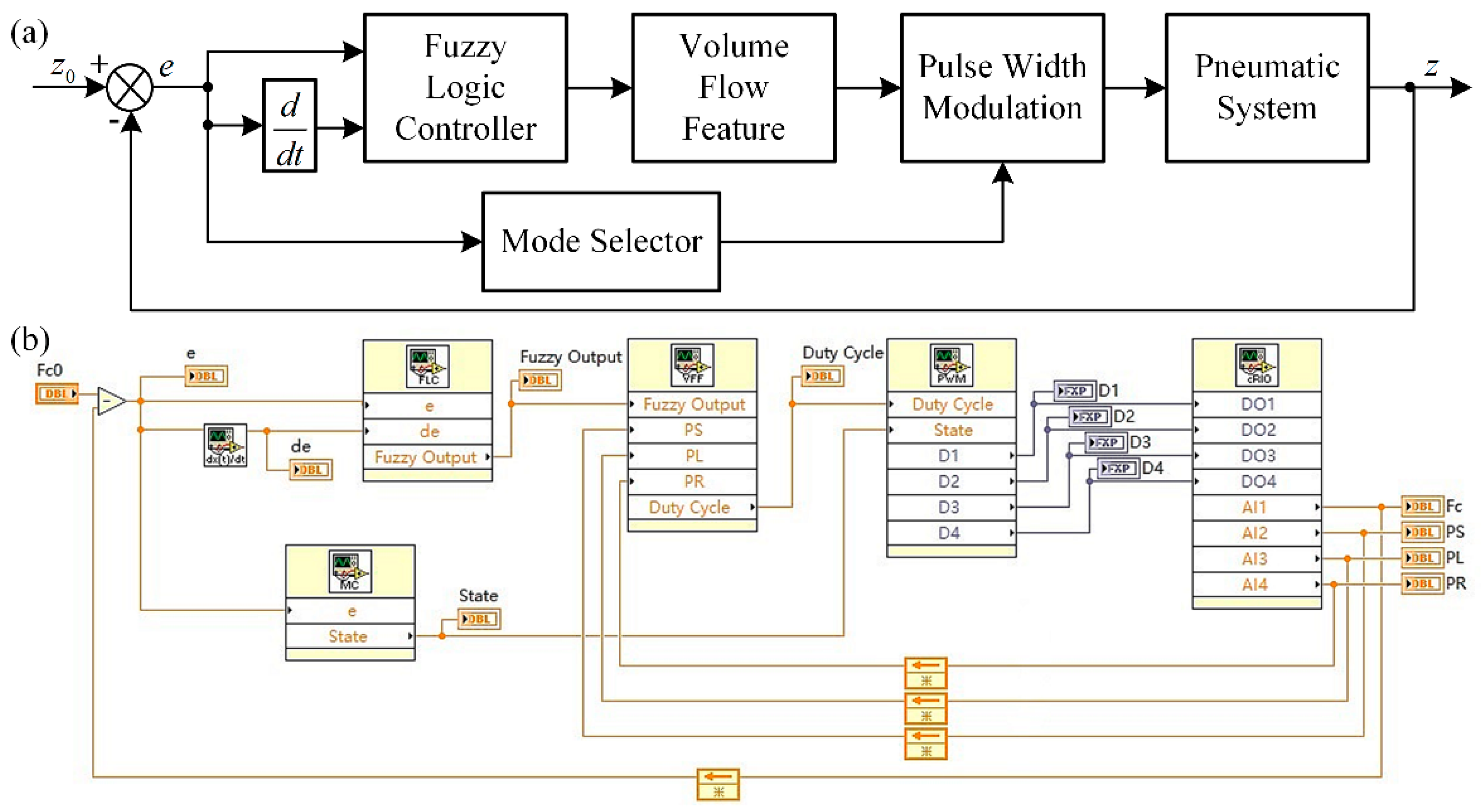
3. Controller Design for the Force Tracking System

In total, four on-off valves are used in the final experiment. Two valves are installed as the inlet valve, and two valves are installed as the outlet valve. The valves are all controlled by control signals from the digital controller. Three pressure sensors are set in the system. The first one is linked to the air supply, the second one is linked to the left chamber of the cylinder, and the third one is linked to the right chamber of the cylinder. A force sensor is installed between the right end of the spring and steel bracket. As shown in Figure 9, the rod of the cylinder is in the leftmost position, and this position is set as the initial position of the force tracking system. In this position, the spring is adjusted to the initial state with no pre-tension, and the output force of the rod is 0 N. According to Newton’s second law of motion, the dynamics of the rod (cylinder) can be written as:
F c F s + F o u t = M a
where F c is the force of the rod, F s is the force of the spring, F o u t is the force caused by the atmosphere acting on the rod, M is the total payloads including the rod, the connector between the spring and the rod, and the spring, and a is the acceleration of the rod. The direction of the acceleration is represented by the arrow in Figure 9. F o u t is small enough to be ignored in this research.
After introducing the entire volume flow feature, an improved volume flow control method is proposed in this section to use the fuzzy logic control. In the previous work of Pipan M. and Herakovič N. [22], bilinear interpolation and a PID controller are used. Polynomial fitting is tested in their work and abandoned in the end. In our work, we initially use the segmented, polynomial fitting method to process the data. At the same time, we develop a new method for calculating the duty cycle which is completely different from the original method. By designing this method, the raw data of the volume flow is able to be combined with the classic fuzzy logic controller. The block diagram of the control scheme is shown in Figure 10a. The fuzzy logic controller is set before the volume flow feature module to generate a proper volume flow percentage value with the input of force error and force error rate. The volume flow feature module converts the volume flow percentage value to a certain duty cycle value. A mode selector is also introduced to improve the control performance. With the mode selector, the action of each on-off valve is decided precisely. Figure 10b is the real program in Labview. Each block represents a ‘sub vi’ which is a user-defined function. FLC, volume flow fitting (VFF), mode controller (MC), and PWM block represent the corresponding function. The cRIO block represents the real embedded controller. Four digital outputs (DOs) are defined for the four valves, and four analog inputs (AIs) are defined for the four sensors. As shown in Figure 10b, they constitute the real closed-loop control system.

3.1. Improved Volume Flow Control Method

As shown in Figure 10, the volume flow feature module is set after the fuzzy logic controller. For this module, three major parameters are the volume flow, duty cycle, and pressure difference. As the purpose of the module is to generate a proper duty cycle for the valve, the input parameter should be decided between volume flow and pressure difference. If the pressure difference is used as the input, it will be difficult to decide the volume flow in the following control process. So the volume flow is set as the input of the module. Both units of volume flow (input parameter) and duty cycle (output parameter) are percentage (%), as normalized data are much easier to be utilized by other modules. The unit of the pressure difference is still MPa since it is only an intermediate value. In order to use the fuzzy logic controller, the collected data which are shown in Figure 8 must be fitted. A segmented, polynomial fitting method is adopted here. The data are first divided into two parts by the duty cycle: 0 t p 10 and 10 < t p 100 . Then they are individually fitted using the fourth-order polynomial fitting equation:
t p = a 0 V % 4 + a 1 V % 3 + a 2 V % 2 + a 3 V % + a 4
where V % is the normalized volume flow. The polynomial fitting curve is shown in Figure 11. In Table 1, the coefficient of determination, R 2 , and the root mean square error (RMSE) are used to determine the accuracy and goodness of the fitting. R 2 usually ranges from 0 to 1, and the closer R 2 is to 1 means the fitting curve is closer to the original data. RMSE usually represents the differences between the fitting curve and the original data. For the duty cycle 0 t p 10 , only one value of RMSE is larger than 1, and other results are quite good for fitting. For the duty cycle 10 < t p 100 , all the values of R 2 are very close to 1, and the values of RMSE are mostly lower than 5. The highest value of RMSE is 5.562 when Δ P is 0.1 MPa. Overall, the total results of the fitting are good enough for the fuzzy logic controller.
Then the output duty cycle, t p , minimum duty cycle, t p m i n , and maximum duty cycle, t p m a x for each valve can be calculated. The pressure difference for each valve can be described as:
{ Δ P a = P S P L Δ P b = P L P a t m Δ P c = P S P R Δ P d = P R P a t m
where Δ P a , Δ P b , Δ P c , and Δ P d are the pressure difference of the left inlet valve, left outlet valve, right inlet valve, and right outlet valve, P S , P L , and P R are the pressure of the air supply, left chamber of the cylinder, and right chamber of the cylinder. As the fitting may cause some serious change to the minimum and maximum pulse width, we still use the original measuring data to calculate the minimum and maximum duty cycle. Then the minimum duty cycle t p m i n and maximum duty cycle t p m a x can be directly calculated from linear interpolation using the normalized data in Figure 6 and Figure 7. The method for calculating the output duty cycle t p is shown in Figure 11c. Assume that the two pressure differences which are closest to the current pressure difference Δ P are Δ P l and Δ P r , then the corresponding duty cycles t p l and t p r can be calculated from linear interpolation with the volume flow V % from the fuzzy logic controller. The output duty cycle t p can be calculated by:
t p = t p l + ( Δ P Δ P l ) ( t p r t p l ) Δ P r Δ P l
For t p , a limiter is applied to ensure that it does not exceed the maximum or minimum range:
t p m i n t p t p m a x

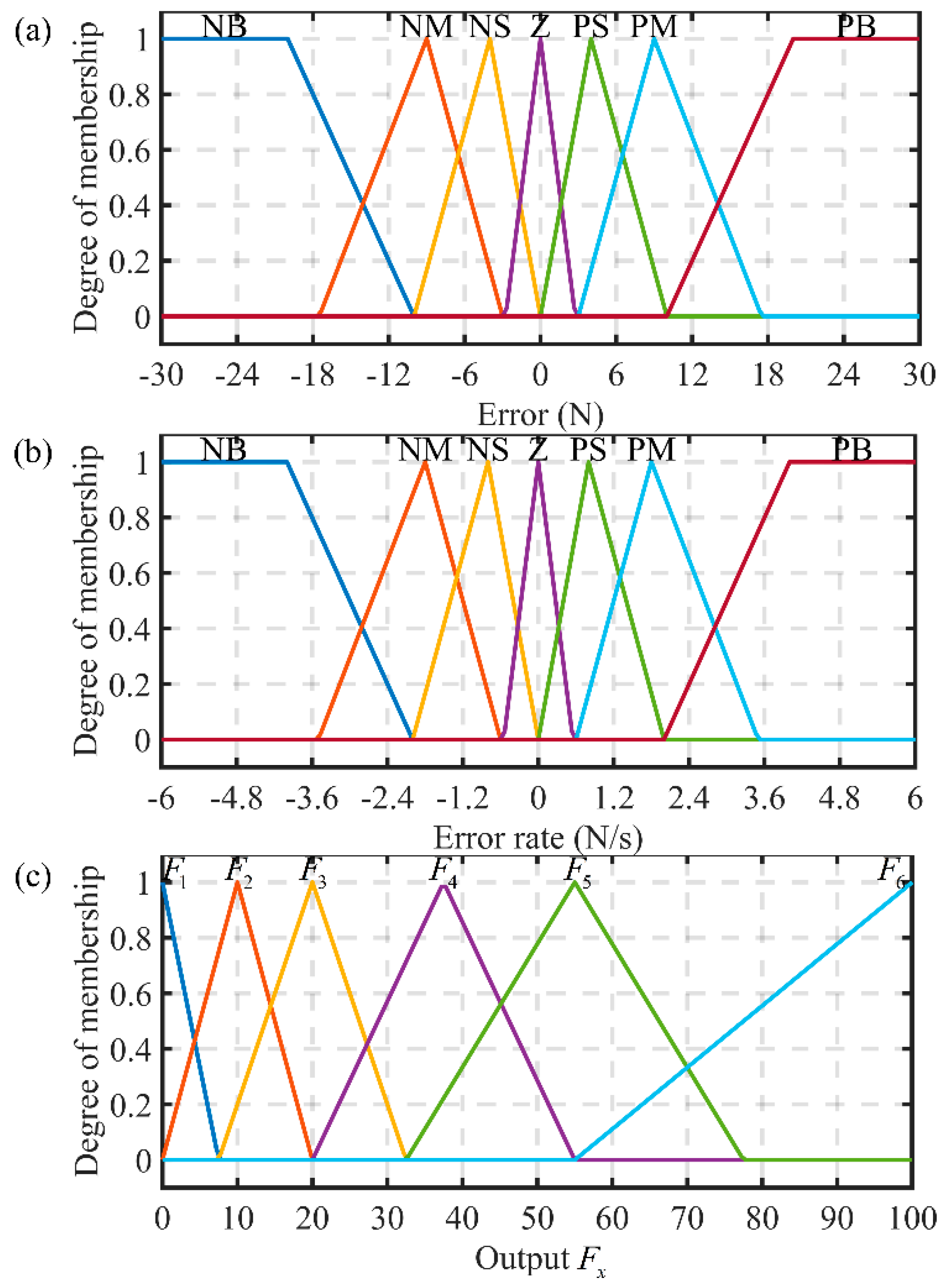
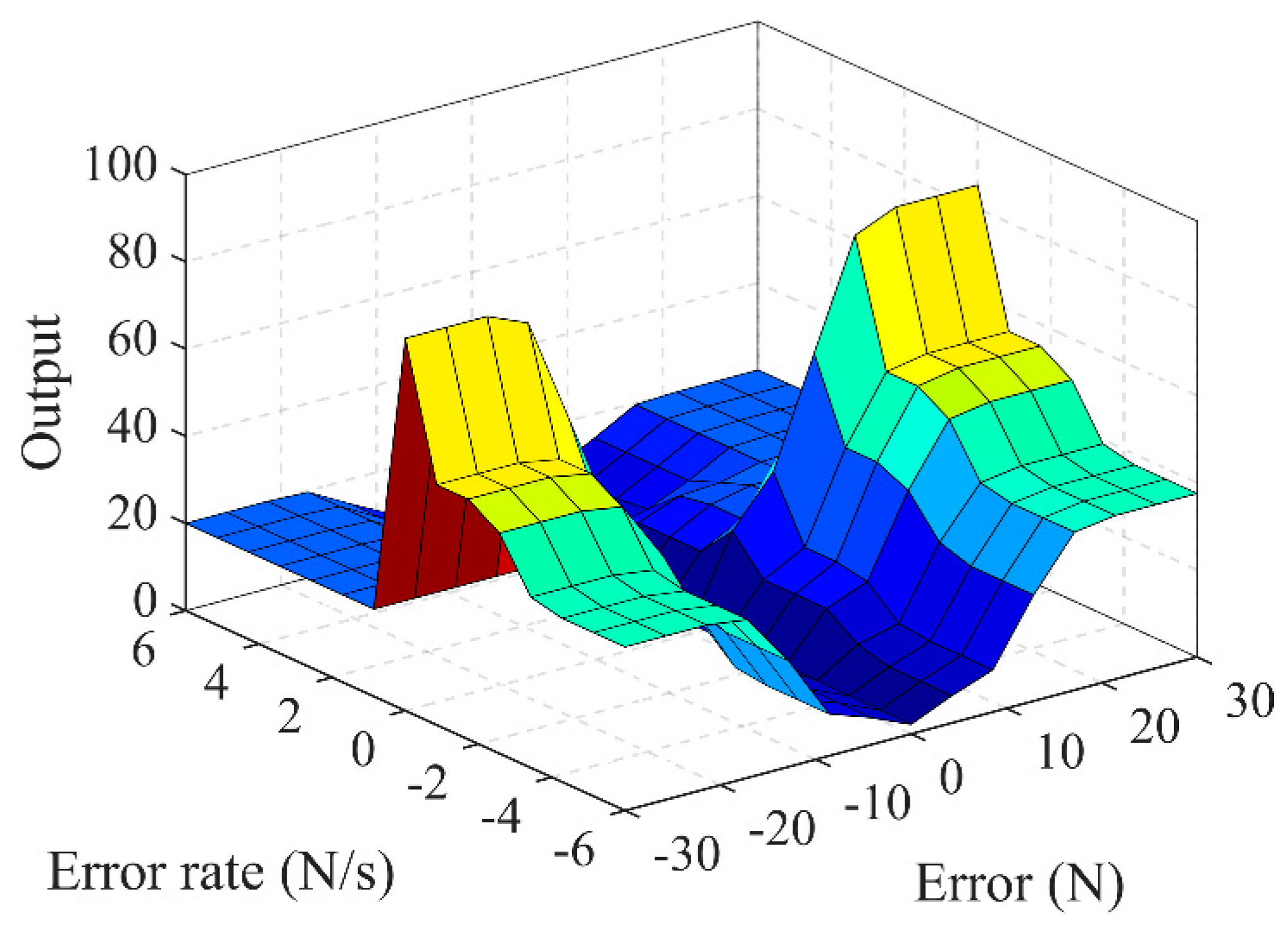
3.2. Fuzzy Logic Controller

A fuzzy logic controller is designed for this highly nonlinear system. The designed fuzzy controller is Mamdani type [31,32] where the input and output are all linguistic variables. The force error e (the difference between the reference force and the measured force) and the force error rate e ˙ (the time derivative of e ) are two input variables, and the output variable F x represents the normalized volume flow V % . The force error is defined as:
e = F c 0 F c
where F c 0 is the force reference, and F c is the measured force of the cylinder. The fuzzy logic controller is composed of four parts: knowledge base, fuzzifier, fuzzy inference engine and defuzzifier [32,33]. The knowledge base is composed of a set of IF-THEN rules K j . The rule form is:
K j :   IF   e   is   A 1 j   and   e ˙   is   A 2 j   Then   F x   is   B j
where j = 1 , 2 , , K , A 1 j , A 2 j , and B j are the linguistic variables. The fuzzifier is the element that connects the numerical input values and the fuzzy inference engine. It converts the real input values into the fuzzy sets of the membership functions. The fuzzy inference engine (FIE) is applied to transfer the fuzzy sets of the membership functions into the fuzzy outputs by using the IF-THEN rules [33]. In our design, the minumum for T-norm (AND), maximum for S-norm (OR), minimum implication method and maximum aggregation method are applied for the FIE. The defuzzifier is utilized to map the fuzzy outputs into real outputs. Center of gravity is chosen as the defuzzification method, and it has the advantage of simplicity and fast calculation. The membership functions of the input variable error, input variable error rate, and output variable, F x , are shown in Figure 12. All the linguistic variables used in this controller are listed in Table 2. NB, NM, NS, Z, PS, PM, and PB represent negative big, negative medium, negative small, zero, positive small, positive medium, and positive big, respectively.
For the input variables, triangular and trapezoidal-shaped functions are used. Different types of membership functions will greatly alter the control performance. The triangular functions occupy the central part of the membership functions. The width of the triangular function gradually widens from the middle to the sides. This is due to the fact that the most sensitive actions usually appear when the error or error rate is near zero. In the middle part of the membership function, the control action is slightly more gentle. Then trapezoidal-shaped functions are utilized when the absolute value of the error or error rate is quite large. It will help reduce the concussion both during the start and end of the control. The level parts also help the system maintain the largest control action when the error or error rate is extremely large or small. The value range of the input variables is chosen by the experiments. The value of error ranges from −30 N to 30 N, and the value of error rate ranges from −6 N/s to 6 N/s. However, for the output variable F x only triangular functions are selected. It is not symmetrical as only positive values are needed for the output. The value of output ranges from 0 to 100. It represents the volume flow percentage with the unit of %. The narrowest triangular function is set near 0 for the most sensitive response.
The fuzzy rules are completely asymmetrical due to the system nonlinearity. As shown in Figure 9, the rod of the cylinder can not move leftward at the initial state. During the motion, it is easier for the rod to move leftward due to the leftward force produced by the spring and the strong compressibility of air. The fuzzy rules are listed in Table 3. Every rule is designed based on the real experimental results. The lowest output is used when the error is Z to ensure the smallest motion when the error is approaching zero. This will also help avoid the overshoot when the force is near the reference. When the error is NS or PS, the lowest output is maintained when the absolute value of the error rate is big (NB or PB). In this state, the rod is in high velocity, and no large control actions are needed. In other states, the second lowest value of output is used due to the low velocity. When the error is NM or PM, the rules are similarly designed. The largest value of output only appears when the error rate is Z, and error is big (NB or PB). It means that the rod is just about to move, and the largest output will greatly boost the initial reaction. The negative error rate means that the error is reducing according to (8). It also represents that the rod is moving rightward, and the measured force is increasing. So when the absolute value of error is big (NB or PB), the outputs for the negative error rate are selected as F 4 and F 5 . For the positive error rate, the outputs are only F 3 . This is due to the asymmetry of the system, and it will maintain a speed balance for moving left and right. Figure 13 shows the control surface.

3.3. Mode Selector

The mode selector shown in Table 4 is designed for two purposes: increasing the response speed and reducing the overshoot. We choose to use the PWM method as the duty cycle for each valve is able to be directly calculated from the controllers mentioned above. When the error is larger than α , the left inlet valve and right outlet valve are set to be open, and other valves are closed. In this mode, the left chamber of the cylinder will be rapidly filled, and the right chamber will be rapidly exhausted. So the rod of the cylinder will move rapidly right, and the force is rising fast. It will increase the response speed by opening two valves at the same time. Similarly, when the error is smaller than α , the right inlet valve and left outlet valve are set to be open, and other valves are closed. In this mode, the right chamber will be rapidly filled, and the left chamber will be exhausted. So the rod of the cylinder will move rapidly left, and the force is decreasing fast. When the error is decreased to a certain range, only one valve is needed to adjust the pressure. In mode 2, the left inlet valve is used to increase the pressure of the left chamber and slightly move the rod right. The force is slightly increasing in this mode. Due to the slow motion and low pressure change, the overshoot will be greatly reduced. Similar to mode 2, mode 4 only uses the right inlet valve to pressure the right chamber. In this mode, the rod will move slightly left, and the force is slightly decreasing. When the error is small enough ( β e β ), all valves are closed. For different reference signals, different values of α and β are chosen. For example, in the step response, a higher value of α (about 1 to 3) is selected to reduce the initial response speed and prevent overshoots. For tracking the triangular wave or sine wave, α can be less than 1 (usually 0.5 to 1). For the value of β , it should be much smaller (usually 0.01) when tracking the triangular wave or sine wave. This setting can make the track more continuous and prevent the cylinder from getting stuck. In the step response, this value can be higher as the reference signal is not changing.

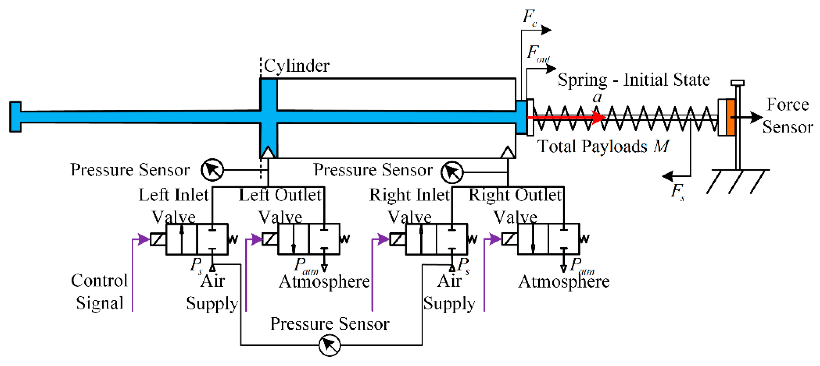
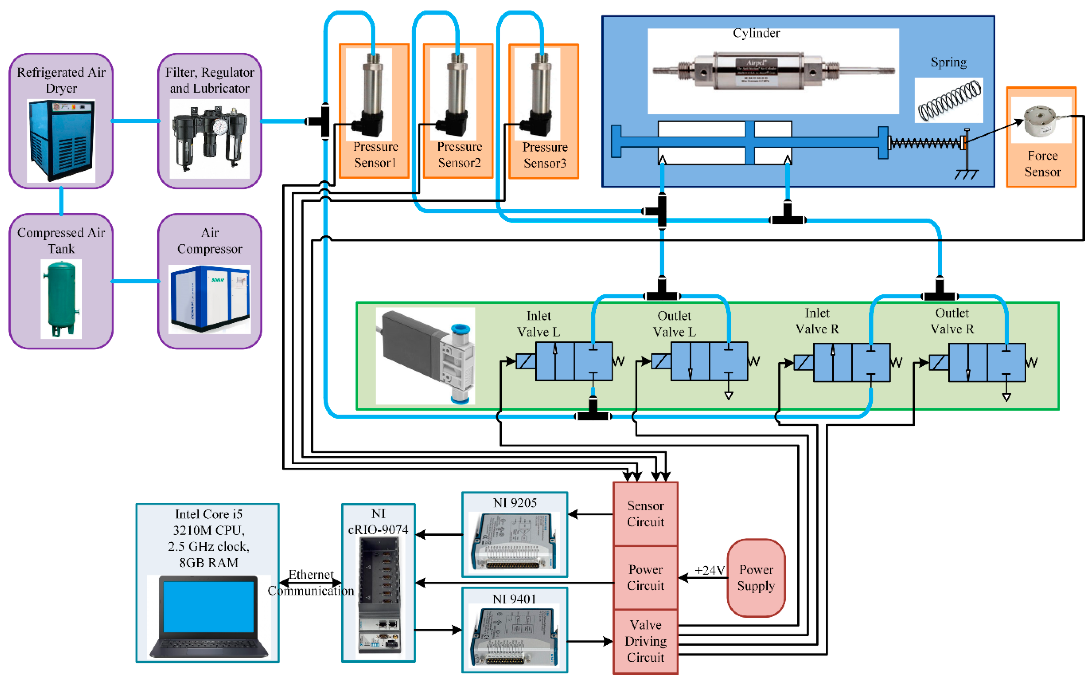
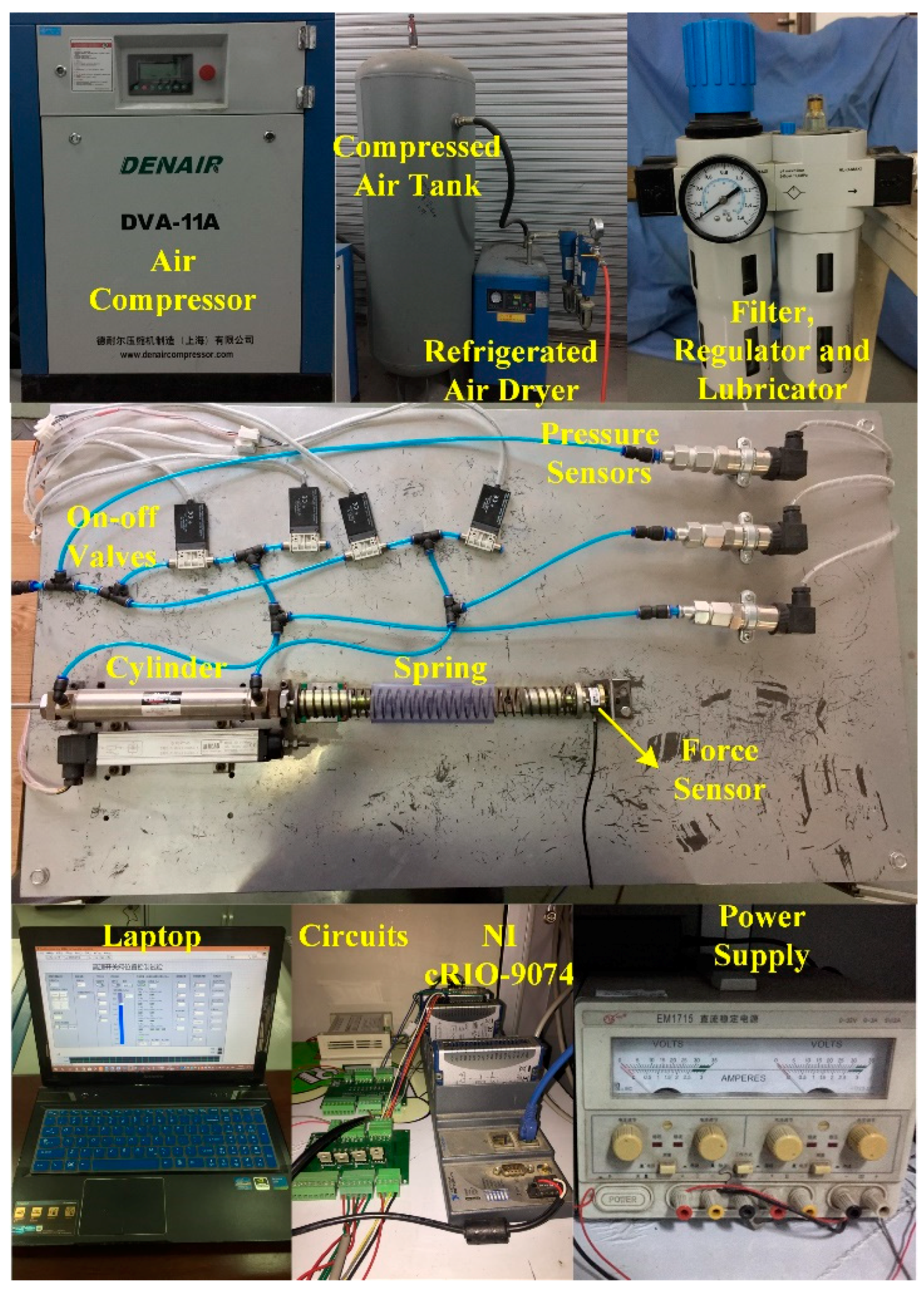
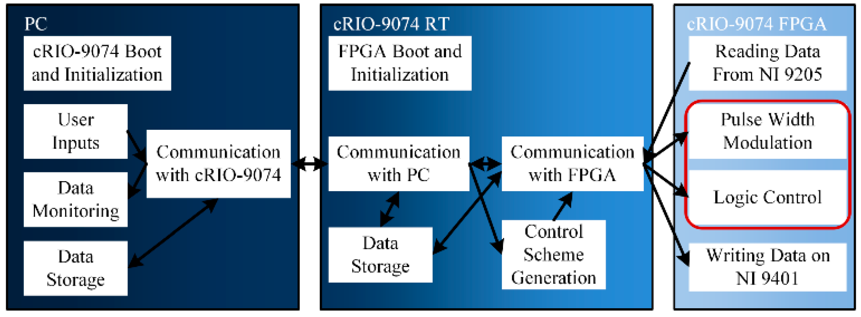
4. Experimental Setup

The final experimental setup is shown in Figure 14. In the pneumatic setup, four on-off valves are applied to control the double-acting, double rod-end, and anti-stiction cylinder (Airpel model M24D100.0D) which is 100 mm in length. The rod diameter is 24mm. A spring which has a length of 150 mm is connected to one rod end of the cylinder. A force sensor (CHINO model ZNHM30) which has the accuracy of 0.3 N and a maximum range of 300 N is attached to the other side of the spring. This force sensor is also fixed on a steel bracket. Some support rods and protective shells are used to keep the whole spring level. Three silicon-diffused pressure sensors (MEACON model MIK-P300) are installed to measure the pressure of the compressed air, and left and right chambers of the cylinder. Other setups are the same as the setups mentioned in Section II. The real pictures of the system are shown in Figure 15. All programs are designed and deployed on NI LabVIEW Pro 11.0, LabVIEW Real-Time (RT) Module 11.0, LabVIEW FPGA Module 11.0, and NI-RIO driver 4.0. The detailed assignments for personal computer (PC), cRIO-9074 RT, and cRIO-9074 FPGA are shown in Figure 16. PWM, logic control, reading data from NI 9205, and writing data on NI 9401 are all executed on the FPGA platform. User inputs and data monitoring are carried out on PC. For the RT platform, the main job is to generate the control scheme and communicate with PC and FPGA. Utilizing the FPGA platform which is extremely reliable in time sequence control guarantees the highly real-time response in the electro-pneumatic control system.

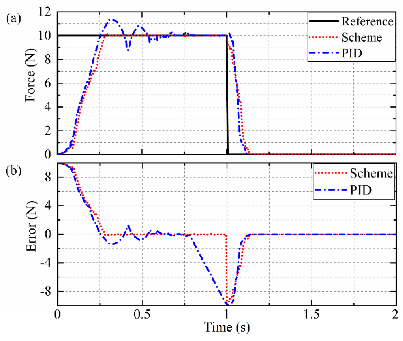
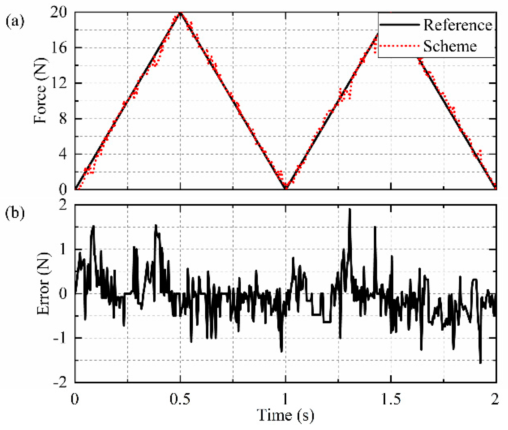
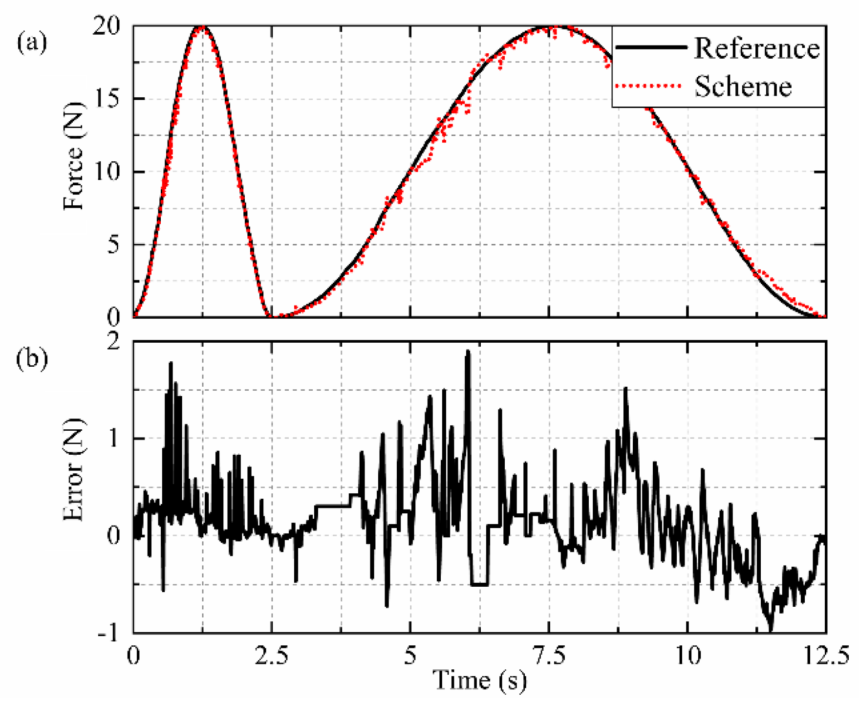
5. Experimental Results and Discussion

One contrast experiment and two tracking experiments are realized on the platform which is shown in Section IV. Several essential system parameters are listed in Table 5.
The first experiment is to compare the control effect of the proposed scheme to the control effect of the conventional PID controller. The PID control algorithm used in the research is expressed as:
u ( t ) = k p e ( t ) + k i 0 t e ( t ) d t + k d e ˙ ( t )
where u ( t ) is the control signal, e ( t ) is the force error, and k p , k i , and k d are the corresponding parameters. The PID parameters are chosen by the Ziegler–Nichols tuning method [34]. The control results are shown in Figure 17. The control parameters are selected as α = 2.5 , β = 0.1 , k p = 1.5 , k i = 0.05 , and k d = 0.001 . 0.141 N (1.41%) overshoot and 0.03 N (0.3%) steady-state error are observed in the results of the proposed scheme. However, for the results of the PID controller, approximately 1.34 N (13.4%) overshoot and 0.34 N (3.4%) steady-state error are found. The settling time of the proposed scheme (0.304 s) is also much smaller than the settling time of the PID controller (0.828 s). The contrast experiment indicates that the proposed scheme is able to reduce the overshoot and increase the response speed indeed. The input signal of the PID controller is the force error and the output signal is the duty cycle. We add a simple mode selector in the PID controller for four valves. When the error is positive, the left inlet valve and right outlet valve are in control. When the error is negative, the left outlet valve and right inlet valve are in control. However, for such a system with severe asymmetry and nonlinearity, the PID controller obviously cannot achieve good effects.
The second experiment is to track a triangular wave reference with the proposed scheme. The biggest force error is 1.906 N (9.53%), and the average force error is 0.049 N (0.245%). As shown in Figure 18, the force response is able to tightly follow the force reference from 0 to 20 N. The control parameters used in this experiment are α = 0.7 and β = 0.01 .
The third experiment is to track a sine wave reference. There are two different frequencies tested in the experiment: 0.4 Hz and 0.1 Hz. The control parameters used in this experiment are α = 1 and β = 0.01 . The tracking response is shown in Figure 19. The force error ranges from −0.97 N to 1.9 N. The average force error is about 0.123 N. The reference signal can be well tracked with the proposed scheme.
The experimental results demonstrate that the improved volume flow control method with fuzzy logic control is effective for controlling the force control system. There is a total of three major innovations which guarantee high performance. Firstly, the acquired volume flow data are accurate, and the subsequent fitting process also ensures the accuracy of the data. The high-precision volume flow meter, advanced data acquisition card, and FPGA real-time acquisition platform guarantee the accuracy of data collection. Then the coefficient of determination and root mean square error are used to determine the quality of the fitting. Secondly, the volume flow control method is highly combined with fuzzy logic control. The output variable of the fuzzy controller is the normalized volume flow which is also a major parameter of the volume flow feature. Fuzzy rules of the fuzzy controller are written based on the asymmetrical characteristics of the real system. Thirdly, the mode selector ensures the fast response in the initial stages of the movement and low overshoot in steady state. In addition, the FPGA platform also guarantees the accurate signal generation and real-time operation of the proposed scheme. Overall, the experimental results show that the method of using the acquired data instead of the traditional theoretical model is feasible.

6. Conclusions

In this research, an improved volume flow control method with fuzzy logic control was proposed to control four solenoid on-off valves in a force tracking system which has a double acting double-rod-end cylinder driven by compressed air. The volume flow feature was firstly studied by precisely acquiring the volume flow data with several high-precision instruments. Then original volume flow data were completely transformed to normalized data and combined with a specially designed fuzzy logic controller. Additionally, a mode selector was utilized to increase the control performance. At last, the improved volume flow control method with fuzzy logic control was combined with the mode selector and applied in the final experiments.
Three experiments including a contrast experiment were carried out on the FPGA platform to verify the effectiveness of the method. The improved volume flow control method with fuzzy logic control shows great advantages over the traditional PID controller in the first experiment. All the control results including the settling time, overshoot, and steady-state error of the proposed scheme are better than the results of the PID controller. In the experiments of tracking the triangular and sine wave, acceptable tracking performances are observed. The results show that good control performance can still be achieved without using conventional theoretical modeling.

Author Contributions

Conceptualization, Z.L. and R.J.; Data curation, R.J.; Formal analysis, Z.L.; Funding acquisition, Q.W.; Investigation, Z.L.; Methodology, Z.L.; Project administration, Q.W. and X.H.; Resources, Z.L. and R.J.; Software, Z.L.; Supervision, Q.W.; Validation, R.J.; Visualization, R.J.; Writing-original draft, Z.L.; Writing-review and editing, Z.L., R.J., Y.Y. and Z.Z.

Funding

This research was funded by the Fundamental Research Funds for the Central Universities (Grant No. NS2018012), the National Natural Science Foundation of China (Grant No. 51576097), the Nanjing University of Aeronautics and Astronautics Ph.D. short-term visiting scholar project, and the Funding of 2018 Jiangsu-UK 20+20 World-class University Action Plan and Customized Project for Ph.D. Student Research and Training.

Acknowledgments

The authors would like to thank Nanjing University of Aeronautics and Astronautics for its support. The authors are sincerely grateful to all the reviewers for the valuable comments.

Conflicts of Interest

The authors declare no conflict of interest.

Nomenclature

V volume flow [L/s]
P i n absolute input pressure of the valve [Pa]
P o u t absolute output pressure of the valve [Pa]
C d valve discharge coefficient [m3/(s·Pa)]
T 0 stagnation temperature [K]
T i n inlet air temperature of the valve [K]
P c specific pressure ratio
P c r critical pressure ratio
T t PWM control period [s]
f p PWM frequency [Hz]
t p w PWM pulse width [s]
t p PWM duty cycle [%]
Δ P pressure difference [Pa]
P a t m pressure of the atmosphere [Pa]
t p m i n PWM minimum duty cycle [%]
t p m a x PWM maximum duty cycle [%]
F c force of the rod [N]
F s force of the spring [N]
F o u t force caused by the atmosphere acting on the rod [N]
M total payloads [kg]
a acceleration of the rod [m/s2]
V % normalized volume flow [%]
R 2 coefficient of determination
Δ P a , Δ P b , Δ P c , and Δ P d pressure difference of the valves [Pa]
P S pressure of the air supply [Pa]
P L pressure of the left chamber [Pa]
P R pressure of the right chamber [Pa]
Δ P l and Δ P r pressure differences [Pa]
t p l and t p r duty cycles [%]
e force error [N]
e ˙ force error rate [N/s]
F x output variable of the fuzzy logic controller
F c 0 force reference [N]
K j IF-THEN rules
A 1 j , A 2 j , and B j linguistic variables
α and β mode selector parameters
L rod length [m]
Drod diameter [m]
Lsspring length [m]
N number of spring coils
k p , ki, and kdPID controller parameters

References

  1. Zhang, Y.; Li, K.; Wang, G.; Liu, J.; Cai, M. Nonlinear Model Establishment and Experimental Verification of a Pneumatic Rotary Actuator Position Servo System. Energies 2019, 12, 1096. [Google Scholar] [CrossRef]
  2. Lin, Z.; Zhang, T.; Xie, Q. Intelligent real-time pressure tracking system using a novel hybrid control scheme. Trans. Inst. Meas. Control 2018, 40, 3744–3759. [Google Scholar] [CrossRef]
  3. Ahn, K.; Yokota, S. Intelligent switching control of pneumatic actuator using on/off solenoid valves. Mechatronics 2005, 15, 683–702. [Google Scholar] [CrossRef]
  4. Nguyen, T.; Leavitt, J.; Jabbari, F.; Bobrow, J. Accurate Sliding-Mode Control of Pneumatic Systems Using Low-Cost Solenoid Valves. IEEE/ASME Trans. Mechatron. 2007, 12, 216–219. [Google Scholar] [CrossRef]
  5. Taghizadeh, M.; Ghaffari, A.; Najafi, F. Modeling and identification of a solenoid valve for PWM control applications. Comptes Rendus Mécanique 2009, 337, 131–140. [Google Scholar] [CrossRef]
  6. Najjari, B.; Barakati, S.; Mohammadi, A.; Futohi, M.; Bostanian, M. Position control of an electro-pneumatic system based on PWM technique and FLC. ISA Trans. 2014, 53, 647–657. [Google Scholar] [CrossRef] [PubMed]
  7. Noritsugu, T. Development of PWM mode electro-pneumatic servomechanism. II: Position control of a pneumatic cylinder. J. Fluid Control. 1989, 17, 7–31. [Google Scholar]
  8. Jeong, H.S.; Kim, H.E. Experimental based analysis of the pressure control characteristics of an oil hydraulic three-way on/off solenoid valve controlled by PWM signal. J. Dyn. Syst. Meas. Control 2002, 124, 196–205. [Google Scholar] [CrossRef]
  9. Messina, A.; Giannoccaro, N.I.; Gentile, A. Experimenting and modelling the dynamics of pneumatic actuators controlled by the pulse width modulation (PWM) technique. Mechatronics 2005, 15, 859–881. [Google Scholar] [CrossRef]
  10. Zhang, J.; Lv, C.; Yue, X.; Li, Y.; Yuan, Y. Study on a linear relationship between limited pressure difference and coil current of on/off valve and its influential factors. ISA Trans. 2014, 53, 150–161. [Google Scholar] [CrossRef]
  11. Ahn, K.; Lee, B. Intelligent switching control of pneumatic cylinders by learning vector quantization neural network. J. Mech. Sci. Technol. 2005, 19, 529–539. [Google Scholar] [CrossRef]
  12. Bangaru, M.; Devaraj, S. Energy efficiency analysis of interconnected pneumatic cylinders servo positioning system. In Proceedings of the ASME 2015 International Mechanical Engineering Congress and Exposition, Houston, TX, USA, 13–19 November 2015; p. V04AT04A034. [Google Scholar]
  13. Shih, M.C.; Ma, M.A. Position control of a pneumatic rodless cylinder using sliding mode MD-PWM control the high speed solenoid valves. JSME Int. J. Ser. C Mech. Syst. Mach. Elem. Manuf. 1998, 41, 236–241. [Google Scholar]
  14. Hodgson, S.; Le, M.; Tavakoli, M.; Pham, M. Improved tracking and switching performance of an electro-pneumatic positioning system. Mechatronics 2012, 22, 1–12. [Google Scholar] [CrossRef] [Green Version]
  15. Lin, Z.; Zhang, T.; Xie, Q.; Wei, Q. Electro-pneumatic position tracking control system based on an intelligent phase-change PWM strategy. J. Braz. Soc. Mech. Sci. Eng. 2018, 40, 512. [Google Scholar] [CrossRef]
  16. Kunt, C.; Singh, R.A. linear time varying model for on–off valve controlled pneumatic actuators. J. Dyn. Syst. Meas. Control 1990, 112, 740–747. [Google Scholar] [CrossRef]
  17. Barth, E.J.; Zhang, J.; Goldfarb, M. Control design for relative stability in a PWM-controlled pneumatic system. Trans. Am. Soc. Mech. Eng. J. Dyn. Syst. Meas. Control 2003, 125, 504–508. [Google Scholar] [CrossRef]
  18. Pohl, J.; Sethson, M.; Krus, P.; Palmberg, J.O. Modelling and validation of a fast switching valve intended for combustion engine valve trains. Proc. Inst. Mech. Eng. Part I J. Syst. Control Eng. 2002, 216, 105–116. [Google Scholar] [CrossRef]
  19. Lin, Z.; Zhang, T.; Xie, Q.; Wei, Q. Intelligent electro-pneumatic position tracking system using improved mode-switching sliding control with fuzzy nonlinear gain. IEEE Access 2018, 6, 34462–34476. [Google Scholar] [CrossRef]
  20. Hodgson, S.; Tavakoli, M.; Pham, M.; Leleve, A. Nonlinear Discontinuous Dynamics Averaging and PWM-Based Sliding Control of Solenoid-Valve Pneumatic Actuators. IEEE/ASME Trans. Mechatron. 2015, 20, 876–888. [Google Scholar] [CrossRef]
  21. Pipan, M.; Herakovič, N. Volume flow characterization of PWM-controlled fast-switching pneumatic valves. Stroj. Vestn. J. Mech. Eng. 2016, 62, 543–550. [Google Scholar] [CrossRef]
  22. Pipan, M.; Herakovič, N. Closed-loop volume flow control algorithm for fast switching pneumatic valves with PWM signal. Control Eng. Pract. 2018, 70, 114–120. [Google Scholar] [CrossRef]
  23. Fu, H.; Jiang, T.; Cui, Y.; Li, B. Adaptive hydraulic potential energy transfer technology and its application to compressed air energy storage. Energies 2018, 11, 1845. [Google Scholar] [CrossRef]
  24. Li, Y.; Xiong, B.; Su, Y.; Tang, J.; Leng, Z. Particle Swarm Optimization-Based Power and Temperature Control Scheme for Grid-Connected DFIG-Based Dish-Stirling Solar-Thermal System. Energies 2019, 12, 1300. [Google Scholar] [CrossRef]
  25. Ma, Y.; Tao, L.; Zhou, X.; Li, W.; Shi, X. Analysis and Control of Wind Power Grid Integration Based on a Permanent Magnet Synchronous Generator Using a Fuzzy Logic System with Linear Extended State Observer. Energies 2019, 12, 2862. [Google Scholar] [CrossRef]
  26. Rahmat, M.F. Identification and non-linear control strategy for industrial pneumatic actuator. Int. J. Phys. Sci. 2012, 7, 2565–2579. [Google Scholar] [CrossRef]
  27. Salim, S.; Rahmat, M.; Faudzi, A.; Ismail, Z. Position control of pneumatic actuator using an enhancement of NPID controller based on the characteristic of rate variation nonlinear gain. Int. J. Adv. Manuf. Technol. 2014, 75, 181–195. [Google Scholar] [CrossRef]
  28. Shih, M.C.; Hwang, C.G. Fuzzy PWM control of the positions of a pneumatic robot cylinder using high speed solenoid valve. JSME Int. J. Ser. C Mech. Syst. Mach. Elem. Manuf. 1997, 40, 469–476. [Google Scholar] [CrossRef]
  29. Pneumatic Fluid Power—Determination of Flow-Rate Characteristics of Components Using Compressible Fluids—Part 1: General Rules and Test Methods for Steady-State Flow, ISO 6358-1:2013. 2013. Available online: https://www.iso.org/standard/56612.html (accessed on 22 October 2019).
  30. McCloy, D.; Martin, H.R. Static characteristics of valves. In Control of Fluid Power: Analysis and Design, 2nd ed.; Halsted Press: New York, NY, USA, 1980; pp. 159–180. [Google Scholar]
  31. Wang, L. A Course in Fuzzy Systems and Control, 1st ed.; Prentice Hall PTR: Upper Saddle River, NJ, USA, 1997; pp. 55–65. [Google Scholar]
  32. Mendes, J.; Araújo, R.; Sousa, P.; Apóstolo, F.; Alves, L. An architecture for adaptive fuzzy control in industrial environments. Comput. Ind. 2011, 62, 364–373. [Google Scholar] [CrossRef]
  33. Mendes, J.; Araújo, R.; Matias, T.; Seco, R.; Belchior, C. Automatic extraction of the fuzzy control system by a hierarchical genetic algorithm. Eng. Appl. Artif. Intell. 2014, 29, 70–78. [Google Scholar] [CrossRef]
  34. Ziegler, J.G.; Nichols, N.B. Optimum settings for automatic controllers. J. Dyn. Syst. Meas. Control 1993, 115, 220–222. [Google Scholar] [CrossRef]
Figure 1. Measure the volume flow: (a) Procedure; (b) Programming interface; (c) Main program. Pulse width modulation (PWM).
Energies 12 04011 g001
Figure 2. Experimental setup of measuring the volume flow. Central Processing Unit (CPU), RAM (Random Access Memory), National Instruments (NI), and CompactRIO (cRIO).
Energies 12 04011 g002
Figure 3. Standard and normalized results from 0.01 MPa pressure difference using three PWM frequencies: (a) Standard results; (b) Normalized results.
Energies 12 04011 g003
Figure 4. Standard and normalized results from 0.1 MPa pressure difference using three PWM frequencies: (a) Standard results; (b) Normalized results.
Energies 12 04011 g004
Figure 5. Standard and normalized results from 0.3 MPa pressure difference using three PWM frequencies: (a) Standard results; (b) Normalized results.
Energies 12 04011 g005
Figure 6. The minimum pulse width of three different PWM frequencies under different pressure differences.
Energies 12 04011 g006
Figure 7. The maximum pulse width of three different PWM frequencies under different pressure difference.
Energies 12 04011 g007
Figure 8. Normalized volume flow results from eight different pressure difference using a 100 Hz PWM frequency.
Energies 12 04011 g008
Figure 9. Schematic diagram of the force tracking system.
Energies 12 04011 g009
Figure 10. The fuzzy logic controller with volume flow feature. (a) Block diagram; (b)The program in Labview. digital outputs (DOs), and analog inputs (AIs).
Energies 12 04011 g010
Figure 11. Final polynomial fitting of the volume flow feature: (a) 3-D relationship between pressure difference, duty cycle, and volume flow; (b) 2-D relationship between duty cycle and volume flow; (c) Method for calculating the output duty cycle.
Energies 12 04011 g011
Figure 12. Membership functions of the fuzzy logic controller: (a) Input variable error; (b) Input variable error rate; (c) Output variable. negative big (NB), negative medium (NM), negative small (NS), zero (Z), positive small (PS), positive medium (PM), and positive big (PB).
Energies 12 04011 g012
Figure 13. Control surface of the fuzzy logic controller.
Energies 12 04011 g013
Figure 14. Final experimental setup.
Energies 12 04011 g014
Figure 15. Pictures of the real system.
Energies 12 04011 g015
Figure 16. Tasks utilized on PC, cRIO-9074 RT, and cRIO-9074. personal computer (PC), Real-Time (RT), and field programmable gate array (FPGA).
Energies 12 04011 g016
Figure 17. Experimental results of the step response for proposed scheme and conventional proportional–integral–derivative (PID) controller: (a) Force; (b) Force error.
Energies 12 04011 g017
Figure 18. Experimental results of the triangular wave: (a) Force; (b) Force error.
Energies 12 04011 g018
Figure 19. Experimental results of the sinusoidal response: (a) Force; (b) Force error.
Energies 12 04011 g019
Table 1. Goodness of fitting. root mean square error (RMSE).
Δ P   ( MPa ) R 2   ( 0 t p 10 )   RMSE   ( 0 t p 10 ) R 2   ( 10 < t p 100 )   RMSE   ( 10 < t p 100 )
0.010.80631.7880.99970.5943
0.030.96060.76870.99930.9722
0.050.99810.16620.99243.255
0.070.97390.6180.99821.585
0.10.98190.5040.97885.562
0.150.97980.53010.9933.227
0.20.98870.42640.98714.395
0.30.99660.21360.99722.067
Table 2. Linguistic variables for error and error rate.
VariableDefinition
NBnegative big
NMnegative medium
NSnegative small
Zzero
PSpositive small
PMpositive medium
PBpositive big
Table 3. Fuzzy rules.
ErrorError Rate
NBNMNSZPSPMPB
NB F 4 F 5 F 5 F 6 F 3 F 3 F 3
NM F 2 F 3 F 3 F 4 F 3 F 3 F 2
NS F 1 F 2 F 2 F 2 F 2 F 2 F 1
Z F 1 F 1 F 1 F 1 F 1 F 1 F 1
PS F 1 F 2 F 2 F 2 F 2 F 2 F 1
PM F 2 F 3 F 3 F 4 F 3 F 3 F 2
PB F 4 F 5 F 5 F 6 F 3 F 3 F 3
Table 4. Mode selector.
Mode (State) 1   ( α < e ) 2   ( β < e α ) 3   ( β e β ) 4   ( a e < β )
V1 1PWMPWMclosedclosed
V2 2closedclosedclosedclosed
V3 3closedclosedclosedPWM
V4 4PWMclosedclosedclosed
1 V1 is the left inlet valve. 2 V2 is the left outlet valve. 3 V3 is the right inlet valve. 4 V4 is the right outlet valve.
Table 5. System parameters.
SymbolSystem ParametersValue
C d valve discharge coefficient4 × 10−9 m3/(s·Pa)
T 0 stagnation temperature293.15 K
P c r critical pressure ratio0.38
P S pressure of the air supply4 × 105 Pa
P a t m pressure of the atmosphere1 × 105 Pa
L rod length0.1 m
D rod diameter0.024 m
L S spring length0.15 m
N number of spring coils33

