Analytical–Numerical Solution for the Skin and Proximity Effects in Two Parallel Round Conductors


Abstract
:
1. Introduction
- Using approximate analytical expressions—e.g., various approximate formulas for alternating current resistance can be found in [11,12,13] and approximations for inductances are given in [14]; integral equation with current density approximated with finite power series was proposed in [15,16]; multipole expansion with finite number of terms was used in [17].
- Mixing analytical and numerical methods—e.g., Rolicz proposed solving the problem with the Bubnov–Galerkin method in the wires and the method of separation of variables in the surrounding region [24].
2. Methodology
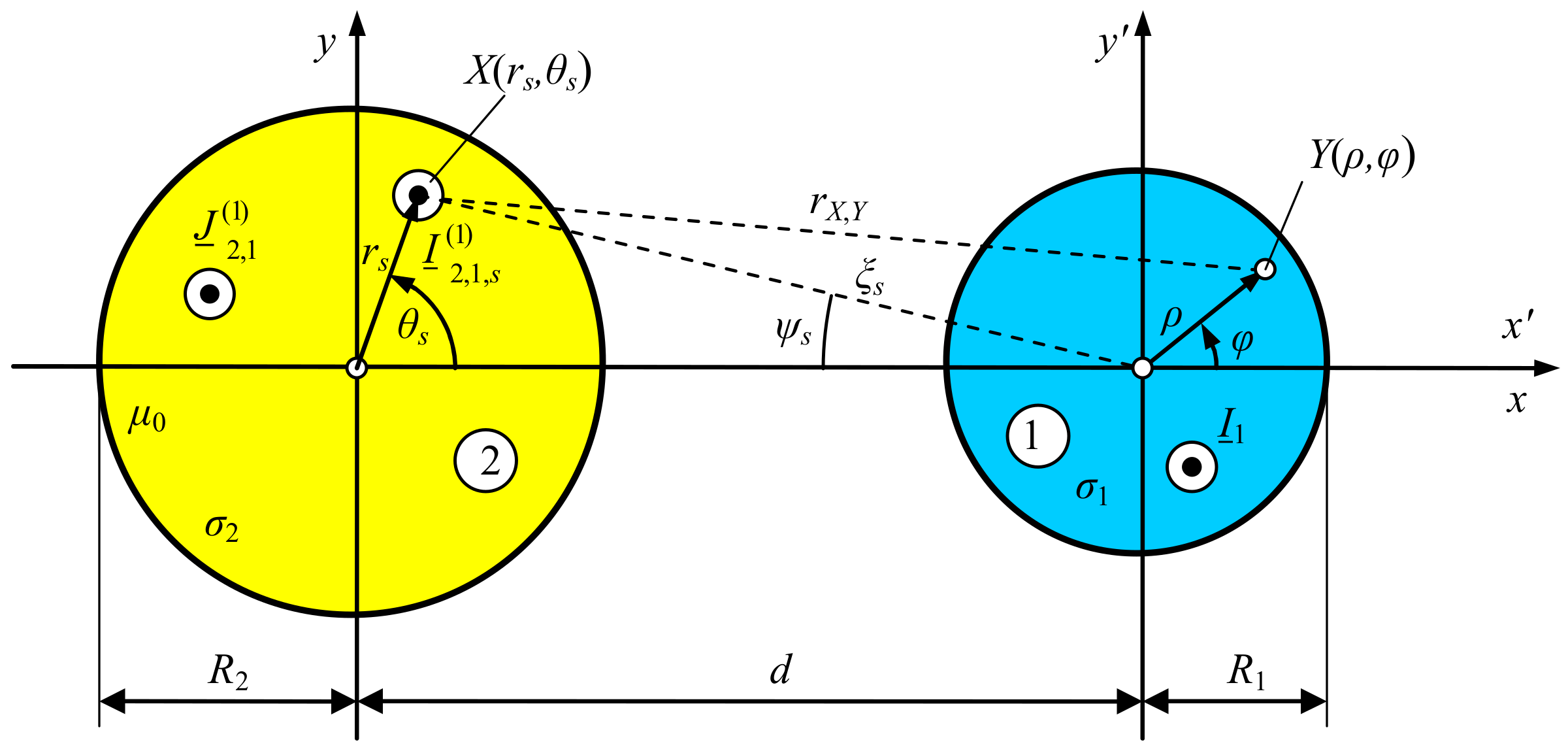
2.1. The Idea of the Method
2.2. The Skin Effect as the Initial Approximation
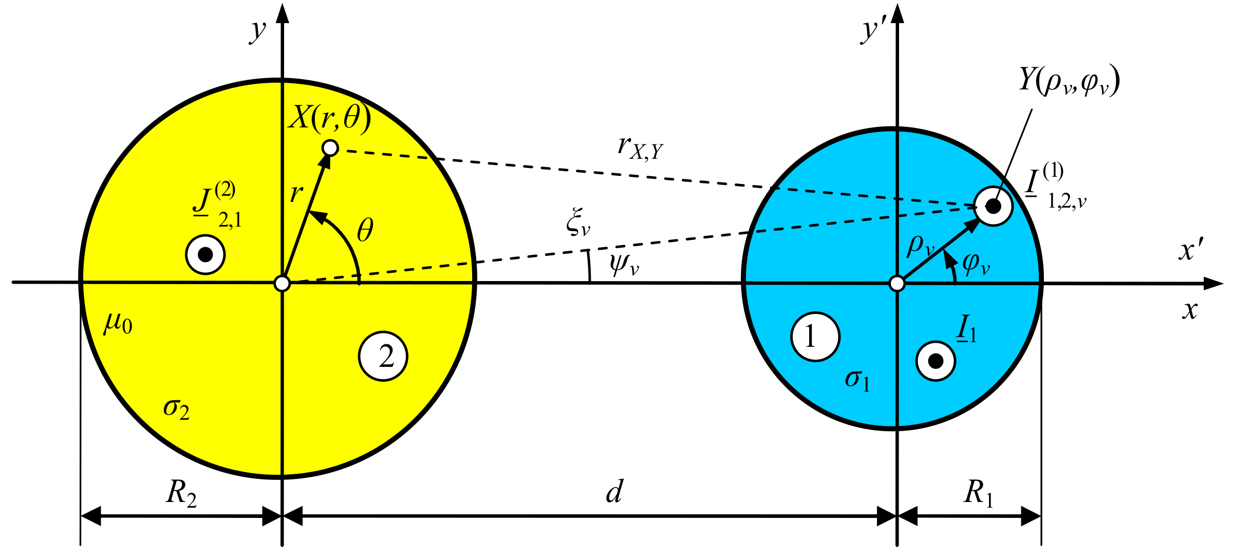
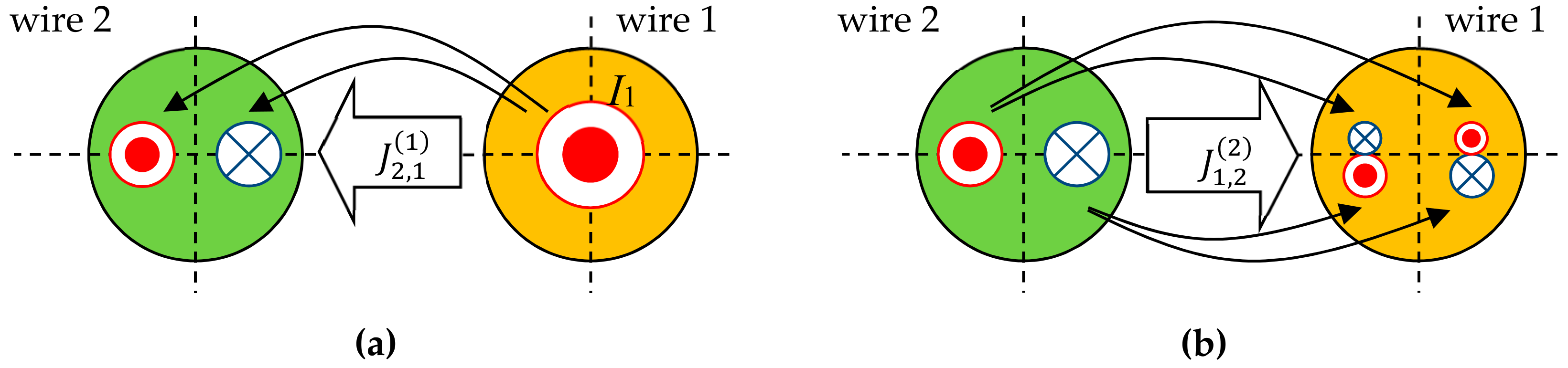
2.3. The First Correction Due to the Proximity Effect
2.4. The Second Approximation
2.5. Discretization of Wires
2.6. Higher Order Reactions
2.7. Algorithm of Calculations
- Given R1, R2, d, σ1, σ2, ω, , calculate necessary values like and
- Divide wires into sectors.
- For (where M is the number of reactions to be taken into account), calculate and using Equations (8b) + (17a), (13a) + (17b), (15b) + (17c), and (14b) + (17d).
3. Results and Discussion
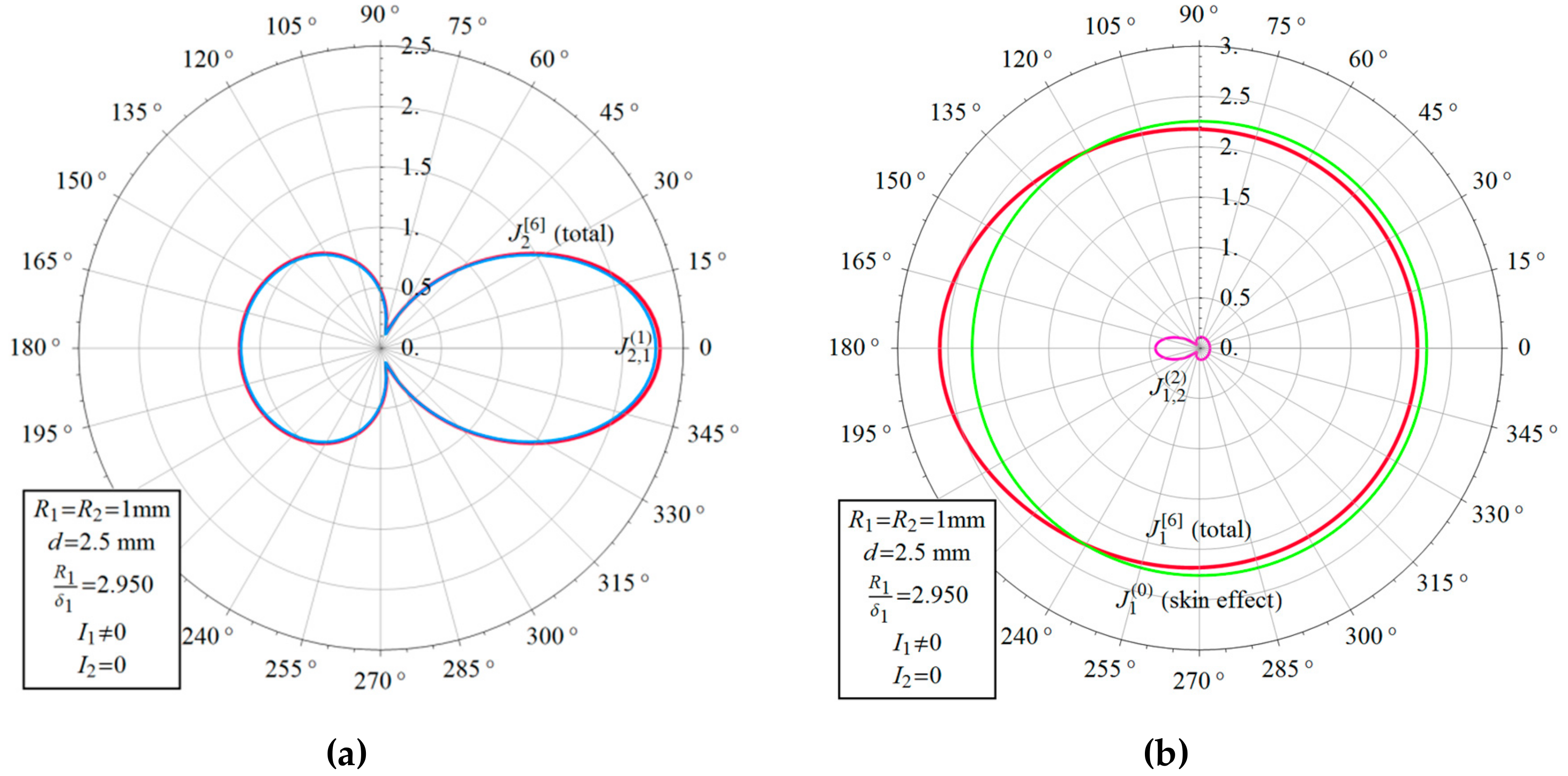
3.1. Numerical Example
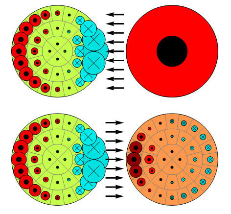
- Case 1: The current in wire 1 is non-zero and in wire 2 is zero;
- Case 2: The currents in both wires are the same; and
- Case 3: The currents in both wires are opposing.
- Each wire is divided into S = V = 100 filaments ( with variable number of sections);
- The relative accuracy of Λ evaluation is (three meaningful digits—see Appendix B); and
- Six reactions were determined.
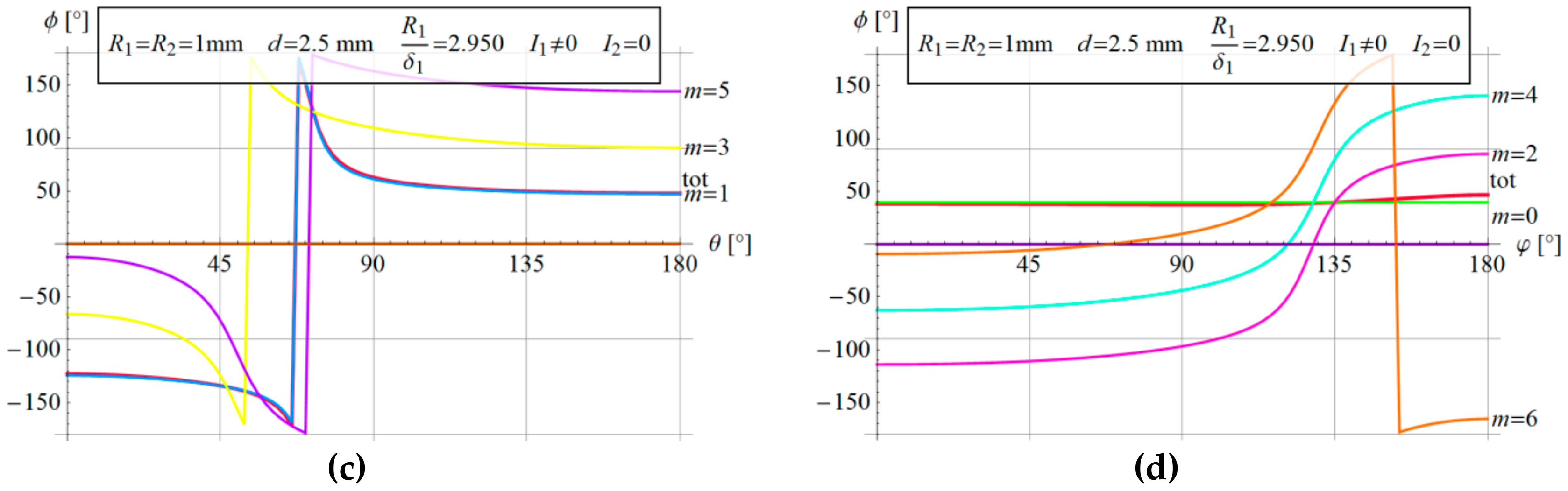
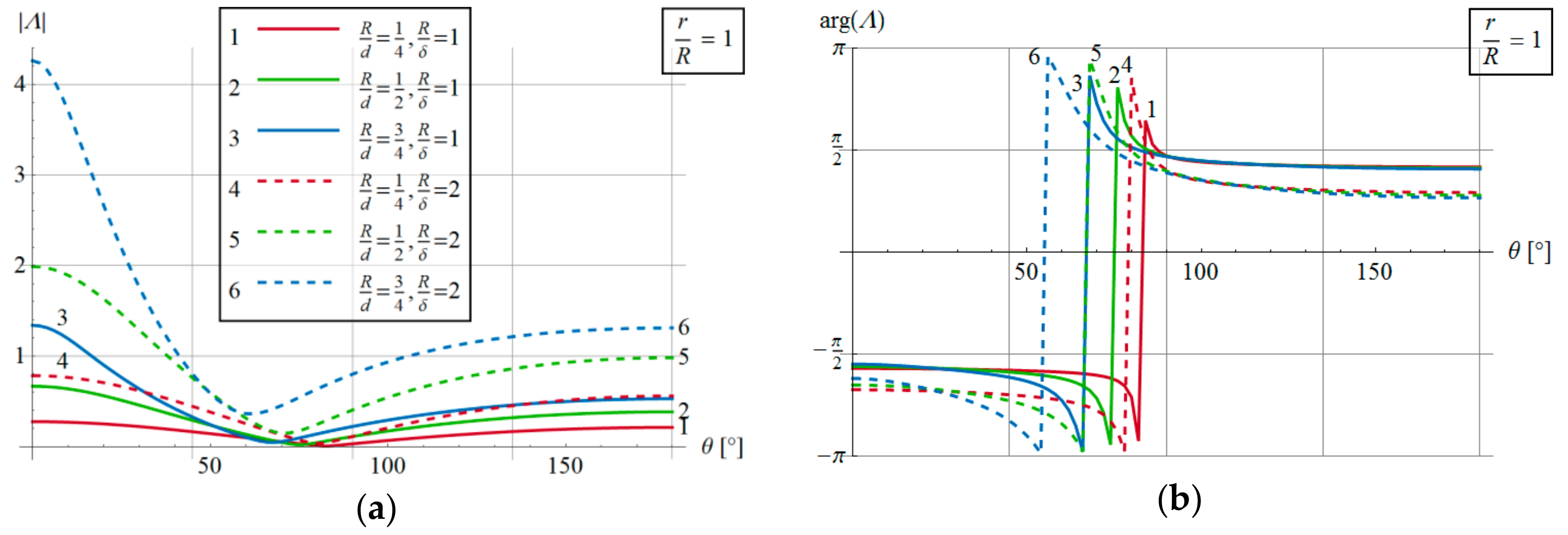
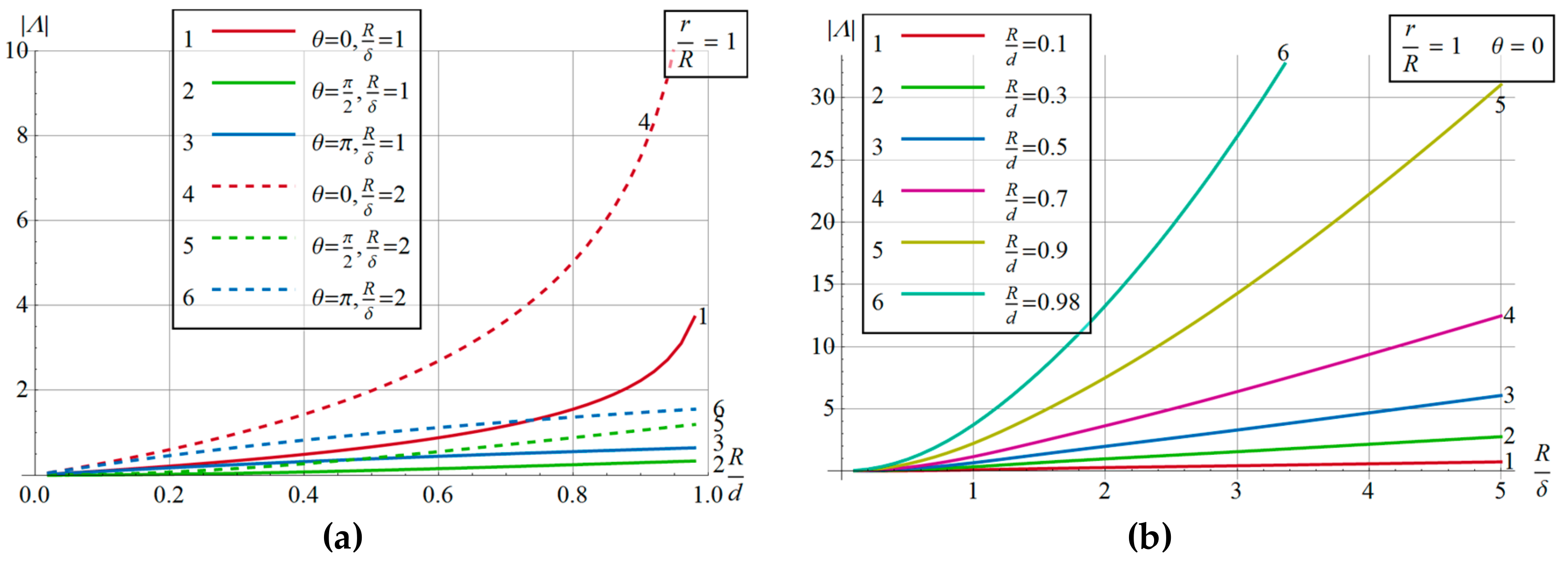
3.2. Analysis of Function Λ
3.3. Analysis of the Successive Reactions
3.4. The Proximity Effect
4. Conclusions
- The results obtained show that there are four parameters directly affecting the current density: R1/d, R2/d, R1/δ1, R2/δ2, which facilitate further analysis.
- The corrections are artificial quantities that can be interpreted as reactions to currents due to previous corrections. They are just auxiliary quantities and cannot be measured—only their total is a real physical quantity.
- In the case of large enough skin depths, reactions 2 and higher can often be neglected without significant loss of accuracy. Therefore, the results with the first correction only are often accurate enough.
- The current density in the wire center is not affected by the corrections—it originates only from the skin effect.
- The current density of an even reaction in a wire is directly proportional to the current in that wire, whereas odd reactions are directly proportional to the current in the neighboring wire.
- The method is not without drawbacks—it cannot be used for non-circular wires and it requires discretization into segments, which introduces uncertainty.
- Further directions of the research can be generalization for a group of more than two wires, for tubular wires, or for wires in conductive environments.
Author Contributions
Funding
Conflicts of Interest
Appendix A

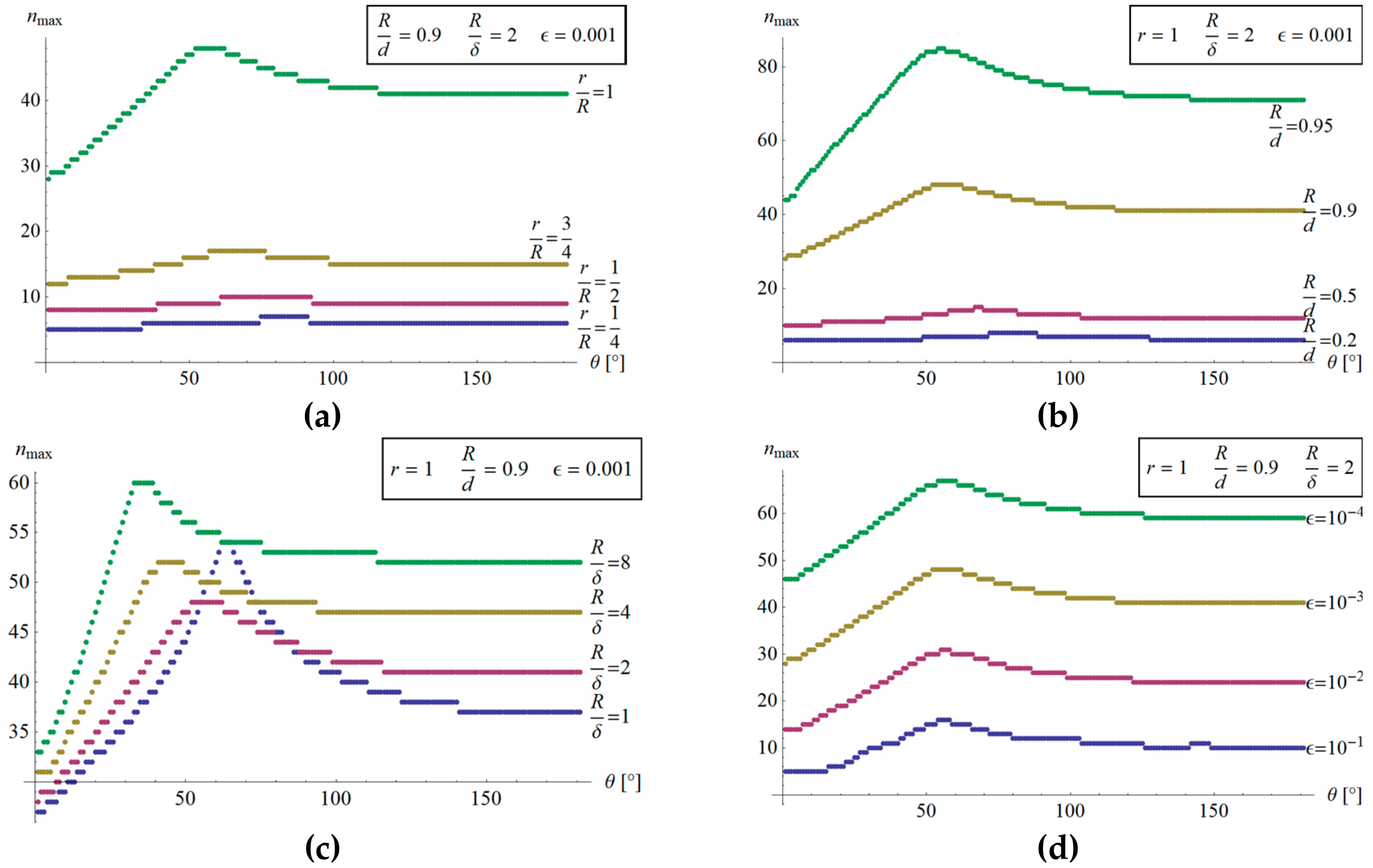
Appendix B
- To obtain an accuracy of three significant digits, the number of terms, , is up to several tens;
- depends on angle and reaches the highest value for ;
- grows with increasing and reaches maximum at ;
- grows with decreasing ; and
- usually grows with decreasing , but surprisingly not for all angles.

References
- Benato, R.; Paoluci, A. EHV AC Undergrounding Electrical Power. Performance and Planning; Springer: London, UK, 2010. [Google Scholar]
- Coufal, O. Current density in two solid parallel conductors and their impedance. Electr. Eng. 2014, 96, 287–297. [Google Scholar] [CrossRef]
- Capelli, F.; Riba, J.R. Analysis of Equations to calculate the AC inductance of different configurations of nonmagnetic circular conductors. Electr. Eng. 2017, 99, 827–837. [Google Scholar] [CrossRef]
- Pagnetti, A.; Xemard, A.; Pladian, F.; Nucci, C.A. An improved method for the calculation of the internal impedances of solid and hollow conductors with inclusion of proximity effect. IEEE Trans. Power Deliv. 2012, 27, 2063–2072. [Google Scholar] [CrossRef]
- Cirino, A.W.; de Paula, H.; Mesquita, R.C.; Saraiva, E. Cable parameter determination focusing on proximity effect inclusion using finite element analysis. In Proceedings of the 2009 Brazilian Power Electronics Conference, Bonito (MS), Brasil, 27 September–1 October 2009; pp. 402–409. [Google Scholar] [CrossRef]
- Dwight, H.B. Proximity effect in wires and thin tubes. Trans. Am. Inst. Electr. Eng. 1923, 42, 850–859. [Google Scholar] [CrossRef]
- Piątek, Z. Method of calculating eddy currents induced by the sinusoidal current of the parallel conductor in the circular conductor. ZN Pol. Śl. Elektryka 1981, 75, 137–150. [Google Scholar]
- Piątek, Z. Impedances of Tubular High Current Busducts; Polish Academy of Sciences: Warsaw, Poland, 2008. [Google Scholar]
- Jabłoński, P. Cylindrical conductor in an arbitrary time-harmonic transverse magnetic field. Prz. Elektrotech. 2011, 87, 49–53. [Google Scholar]
- Filipović, D.; Dlabač, T. Closed Form Solution for the Proximity Effect in a Thin Tubular Conductor Influenced by a Parallel Filament. Serb. J. Electr. Eng. 2010, 7, 13–20. [Google Scholar] [CrossRef]
- Payne, A. Skin Effect, Proximity Effect and the Resistance of Circular and Rectangular Conductors. ©Alan Payne. 2017. Available online: http://g3rbj.co.uk/wp-content/uploads/2017/06/Skin-Effect-Proximity-Loss-and-the-Resistance-of-Circular-and-Rectangular-Conductors-Issue-4.pdf (accessed on 21 July 2019).
- Riba, J.R. Analysis of Equations to calculate AC resistance of different conductors’ configurations. Electr. Power Syst. Res. 2015, 127, 93–100. [Google Scholar] [CrossRef]
- Kim, J.; Park, Y.J. Approximate Closed-Form Equation for Calculating Ohmic Resistance in Coils of Parallel Round Wires With Unequal Pitches. IEEE Trans. Ind. Electron. 2015, 62, 3482–3489. [Google Scholar]
- Aebischer, H.A.; Friedli, H. Analytical approximation for the inductance of circularly cylindrical two-wire transmission lines with proximity effect. Adv. Electromagn. 2018, 7, 25–34. [Google Scholar] [CrossRef]
- Dlabač, T.; Filipović, D. Integral equation approach for proximity effect in a two-wire line with round conductors. Tech. Vjesn. 2015, 22, 1065–1068. [Google Scholar] [CrossRef]
- Filipović, D.; Dlabač, T. Proximity effect in a shielded symmetrical three-phase line. Serb. J. Electric. Eng. 2014, 11, 585–596. [Google Scholar] [CrossRef]
- Brito, A.; Maló Machado, V.; Almeida, M.E.; Guerreiro das Neves, M. Skin and Proximity Effects in the Series-Impedance of Three-Phase Underground Cables. Electr. Power Syst. Res. 2016, 130, 132–138. [Google Scholar] [CrossRef]
- Riba, J.R. Calculation of AC to DC resistance ratio of conductive nonmagnetic straight conductors by applying FEM simulations. Eur. J. Phys. 2015, 36, 055019. [Google Scholar] [CrossRef]
- Riba, J.R.; Capelli, F. Calculation of the inductance of conductive nonmagnetic conductors by means of finite element method simulations. Int. J. Electr. Educ. 2018, 13, 1–23. [Google Scholar] [CrossRef]
- Jabłoński, P. Approximate BEM analysis of time-harmonic magnetic field due to thin-shielded wires. Poznan Univ. Technol. Acad. J. Electr. Eng. 2012, 69, 57–64. [Google Scholar]
- Shendge, A. A study on a conductor system for investigation of proximity effect. J. Electromagn. Anal. Appl. 2012, 4, 440–446. [Google Scholar] [CrossRef]
- Piątek, Z. Self and mutual impedances of a finite length gas-insulated transmission line (GIL). Electr. Power Syst. Res. 2007, 77, 191–201. [Google Scholar] [CrossRef]
- Piatek, Z.; Kusiak, D.; Szczegielniak, T. Electromagnetic field and impedances of high current busducts. In Proceedings of the 2010 International Symposium, Wroclaw, Poland, 20–22 September 2010. [Google Scholar]
- Rolicz, P. Eddy currents generated in a system of two cylindrical conductors by a transverse alternating magnetic field. Electr. Power Syst. Res. 2009, 79, 295–300. [Google Scholar] [CrossRef]
- Piątek, Z.; Baron, B.; Jabłoński, P.; Kusiak, D.; Szczegielniak, T. Numerical method of computing impedances in shielded and unshielded three-phase rectangular busbar systems. Prog. Electromagn. Res. B 2013, 51, 135–156. [Google Scholar] [CrossRef]
- Freitas, D.; Guerreiro das Neves, M.; Almeida, M.E.; Maló Machado, V. Evaluation of the Longitudinal Parameters of an Overhead Transmission Line with Non-Homogeneous Cross Section. Electr. Power Syst. Res. 2015, 119, 478–484. [Google Scholar] [CrossRef]
- Moon, P.; Spencer, D.E. Foundations of Electrodynamics; D. Van Nostrand Company, Inc.: New York, NY, USA, 1960. [Google Scholar]
- Gradshteyn, I.S.; Ryzhik, I.M. Tables of Integrals, Sums, Series and Products, 17th ed.; Elsevier Academic Press: Cambridge, MA, USA, 2007. [Google Scholar]


| Point | Quantity | Case 1 | Case 2 | Case 3 | |||
|---|---|---|---|---|---|---|---|
| Proposed | FEMM | Proposed | FEMM | Proposed | FEMM | ||
| Magnitude | 2.164 | 2.158 | 3.317 | 3.310 | 1.033 | 1.031 | |
| Phase | 38.3 | 37.9 | 41.5 | 41.3 | 27.6 | 27.0 | |
| Magnitude | 2.178 | 2.175 | 2.622 | 2.617 | 1.755 | 1.754 | |
| Phase | 37.5 | 37.1 | 42.0 | 41.7 | 30.8 | 30.3 | |
| (R1, 180°) | Magnitude | 2.578 | 2.566 | 0.517 | 0.502 | 4.869 | 4.850 |
| Phase | 46.7 | 47.1 | –7.1 | –6.2 | 51.7 | 51.8 | |
| (R2, 0°) | Magnitude | 2.311 | 2.302 | 0.517 | 0.502 | 4.869 | 4.850 |
| Phase | –122.9 | –122.8 | –7.1 | –6.3 | –128.3 | –128.2 | |
| (R2, 90°) | Magnitude | 0.482 | 0.481 | 2.622 | 2.617 | 1.755 | 1.755 |
| Phase | 62.7 | 62.8 | 42.0 | 41.7 | –149.2 | –149.7 | |
| Magnitude | 1.164 | 1.162 | 3.317 | 3.309 | 1.033 | 1.032 | |
| Phase | 47.7 | 47.6 | 41.5 | 41.3 | –152.4 | –153.0 | |
© 2019 by the authors. Licensee MDPI, Basel, Switzerland. This article is an open access article distributed under the terms and conditions of the Creative Commons Attribution (CC BY) license (http://creativecommons.org/licenses/by/4.0/).
Share and Cite
Jabłoński, P.; Szczegielniak, T.; Kusiak, D.; Piątek, Z. Analytical–Numerical Solution for the Skin and Proximity Effects in Two Parallel Round Conductors. Energies 2019, 12, 3584. https://doi.org/10.3390/en12183584
Jabłoński P, Szczegielniak T, Kusiak D, Piątek Z. Analytical–Numerical Solution for the Skin and Proximity Effects in Two Parallel Round Conductors. Energies. 2019; 12(18):3584. https://doi.org/10.3390/en12183584
Chicago/Turabian StyleJabłoński, Paweł, Tomasz Szczegielniak, Dariusz Kusiak, and Zygmunt Piątek. 2019. "Analytical–Numerical Solution for the Skin and Proximity Effects in Two Parallel Round Conductors" Energies 12, no. 18: 3584. https://doi.org/10.3390/en12183584