Thermal State of the Blake Ridge Gas Hydrate Stability Zone (GHSZ)—Insights on Gas Hydrate Dynamics from a New Multi-Phase Numerical Model


Abstract
:1. Introduction
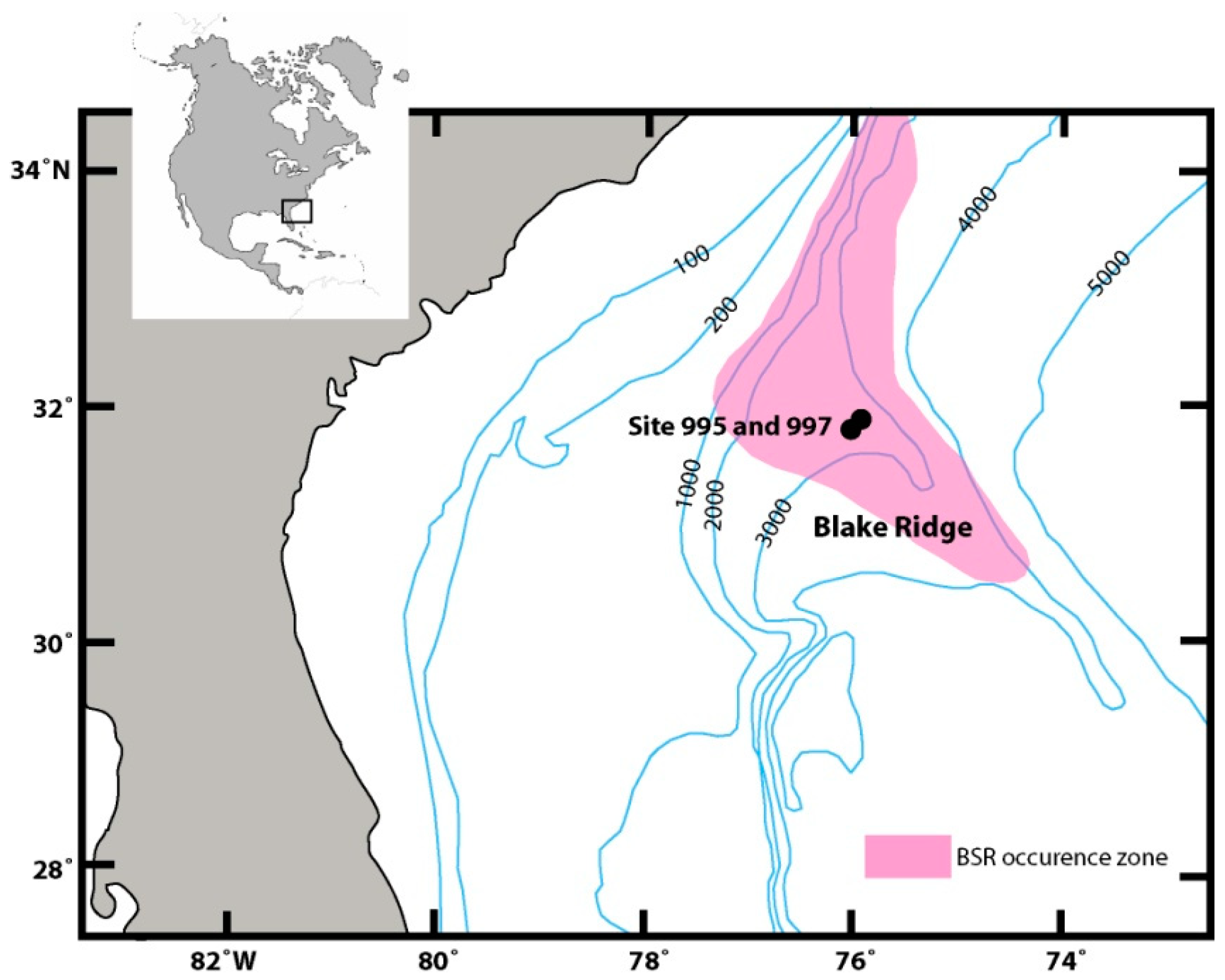
1.1. The Blake Ridge Site Geological Setting and Characterization
1.2. Depth Discrepancy between the Observed BSRs and the Base of the GHSZ at Sites 995 and 997
1.3. Previous Modeling Approaches of the Blake Ridge Site 997
2. Materials and Methods
2.1. Mathematical Model
2.1.1. Introduction
2.1.2. Governing Equations
2.1.3. Source Terms-Bio-Chemical Reactions
2.1.4. Temperature
2.2. Numerical Model
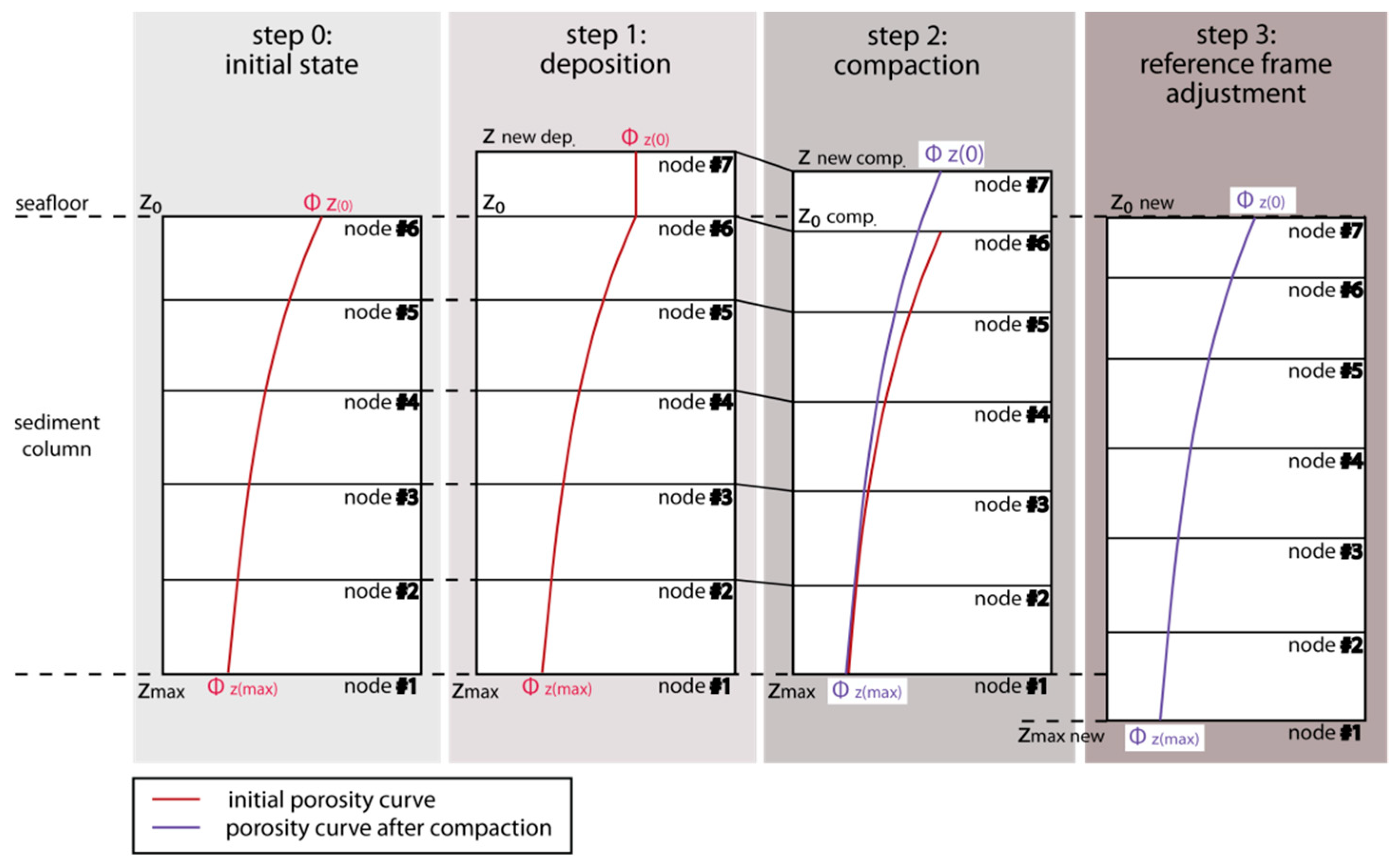
2.2.1. Reference Frame
2.2.2. Initial and Boundary Conditions
2.2.3. Solution Algorithm
3. Results and Discussion

| Scenario | 1 | 2a | 2b | 2c | 3 | 4 | 5 |
|---|---|---|---|---|---|---|---|
| Sources of methane | In-situ POC degradation | In-situ POC degradation | In-situ POC degradation | In-situ POC degradation | In-situ POC degradation | In-situ + Methane flux | In-situ + Methane flux |
| Sedimentation rates | 22 cm∙kyr−1 | Variable | Variable | Variable | Variable | Variable | Variable |
| POC content at the seafloor | 1.6 wt.% | 1.6 wt.% | 1.6 wt.% | 1.6 wt.% | Variable | 1.6 wt.% | Variable |
| Diffusion of dissolved species | - | - | diminished | enhanced | - | - | - |
| Simulation time | 10 Myr | 10 Myr | 10 Myr | 10 Myr | 10 Myr | 10 Myr | 10 Myr |
| Figure with the Results | Figure 3 | Figure 4 | Figure 5 | Figure 6 | Figure 7 | Figure 8 | Figure 9 |


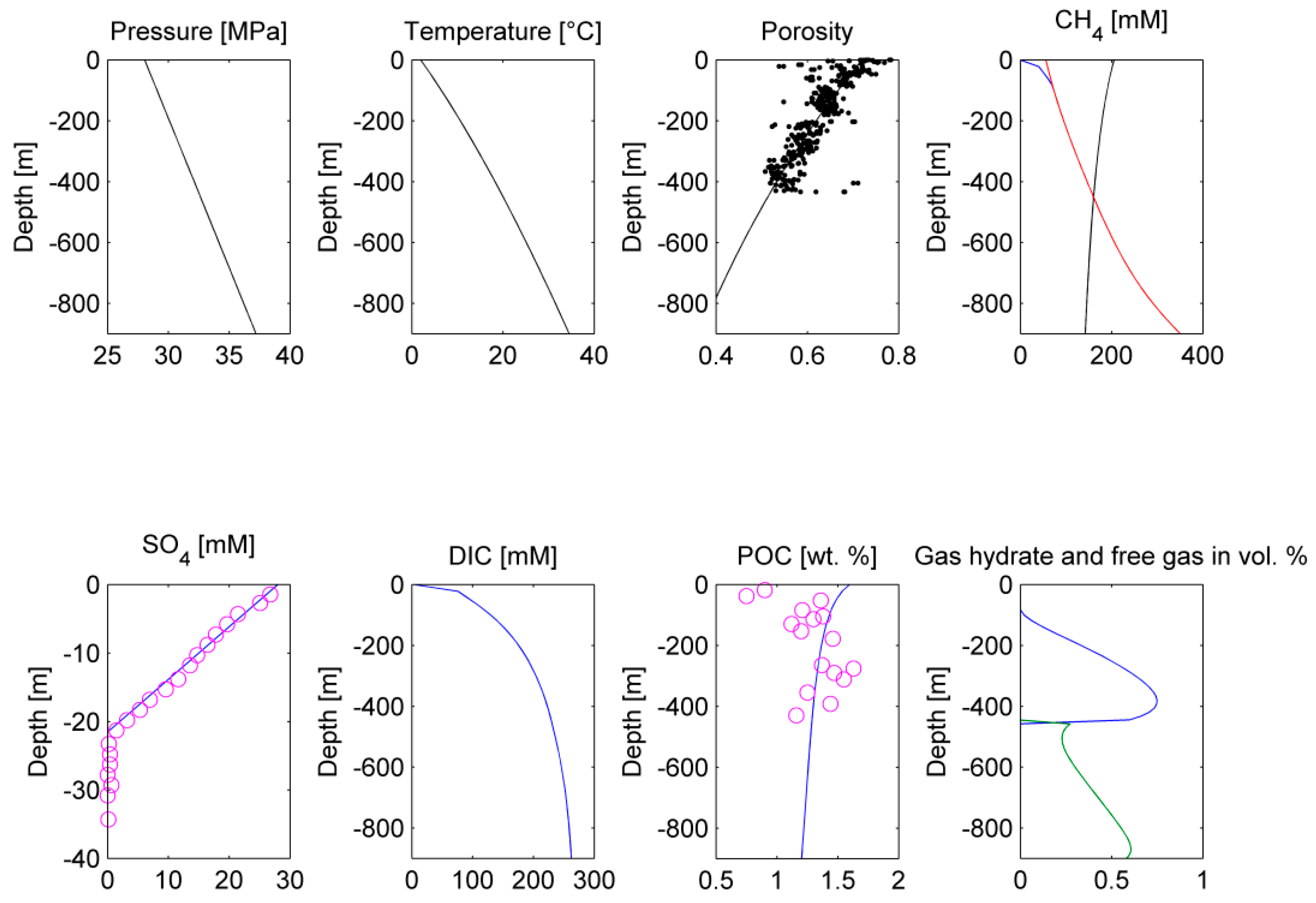
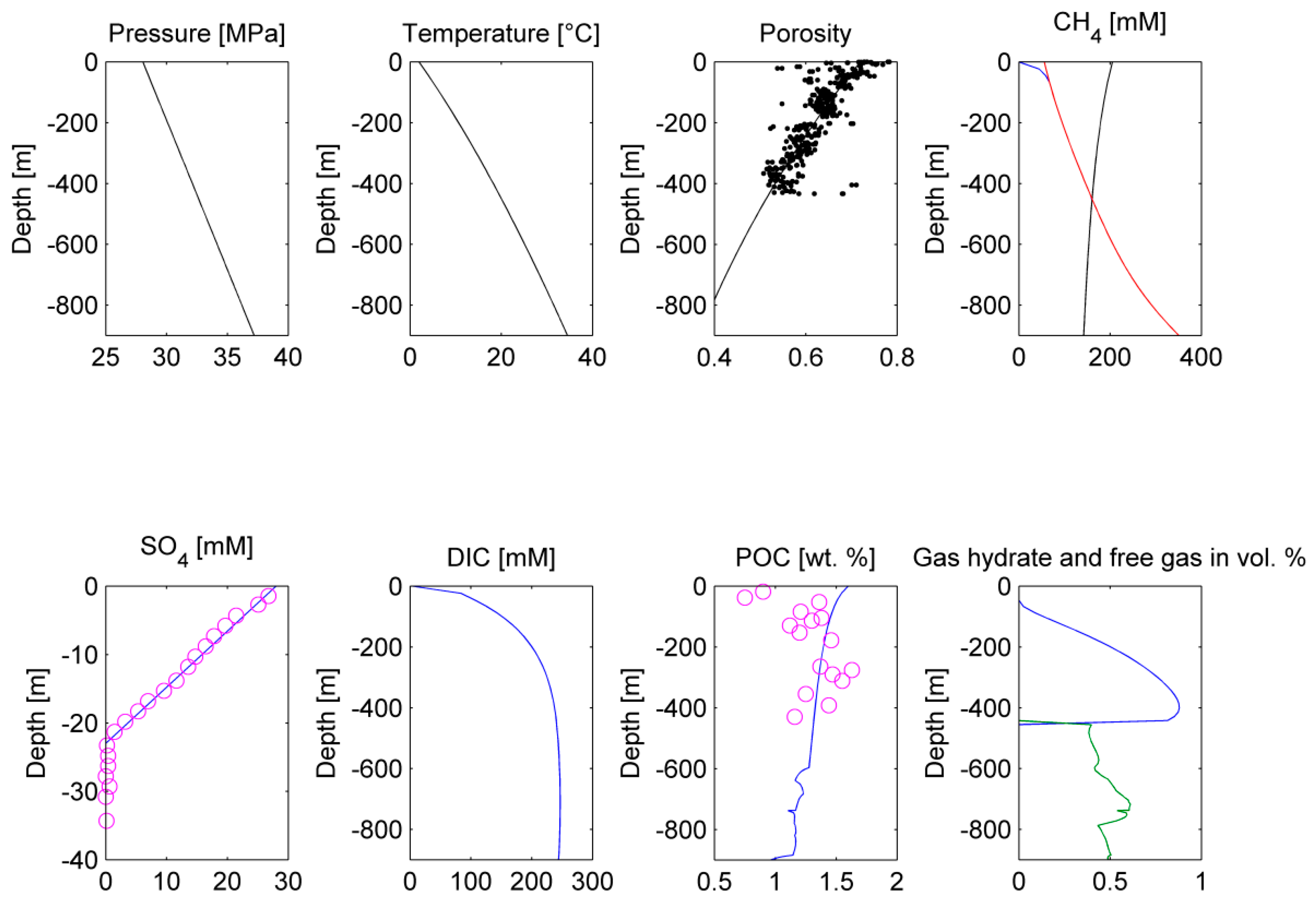
3.1. Scenario 1
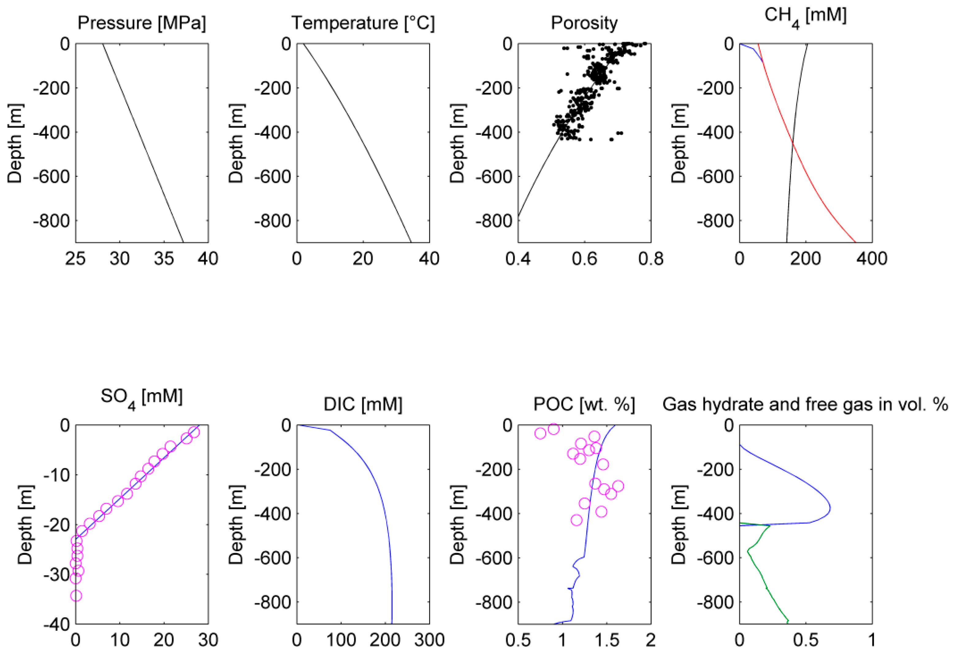
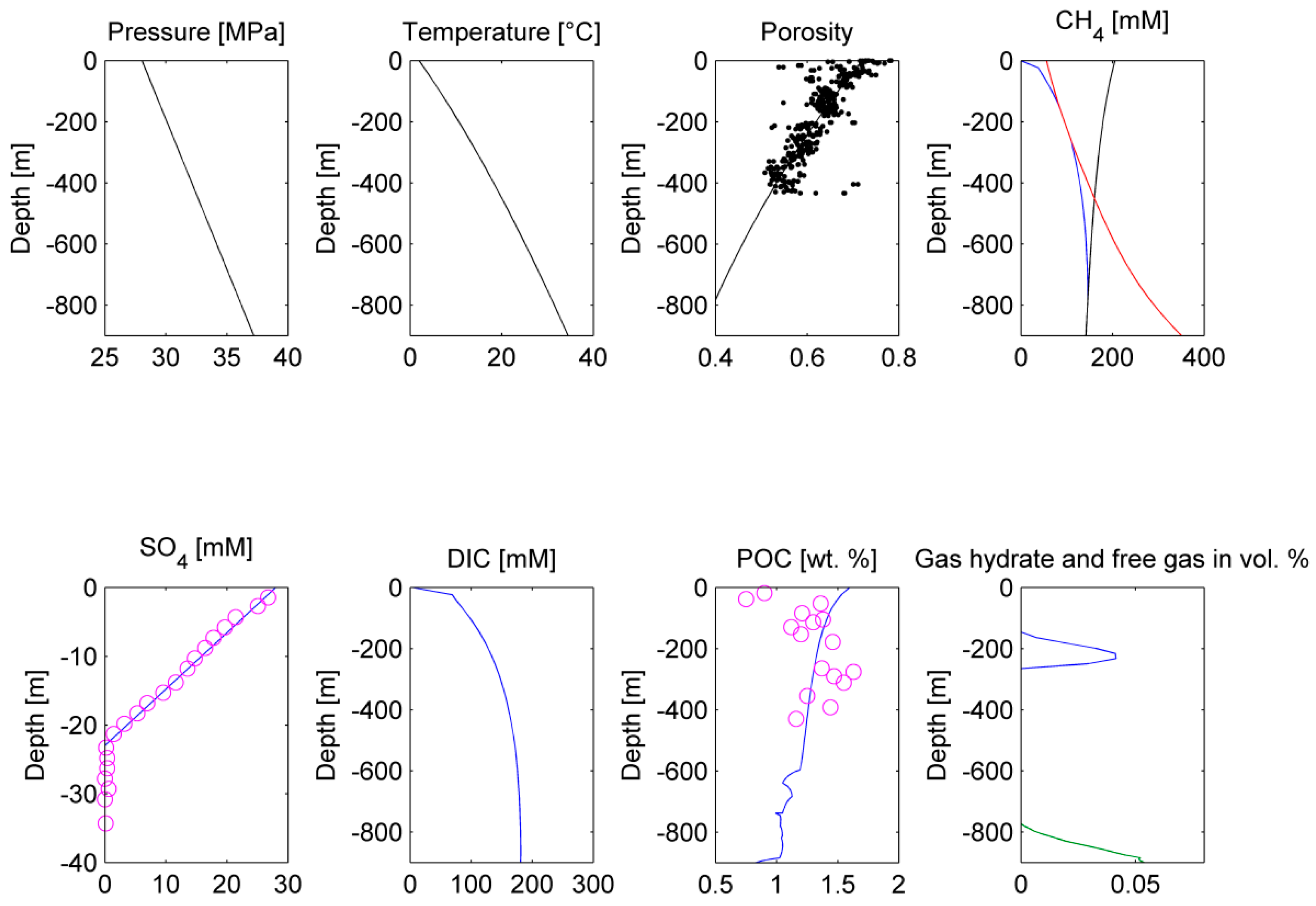
3.2. Scenario 2a%–c
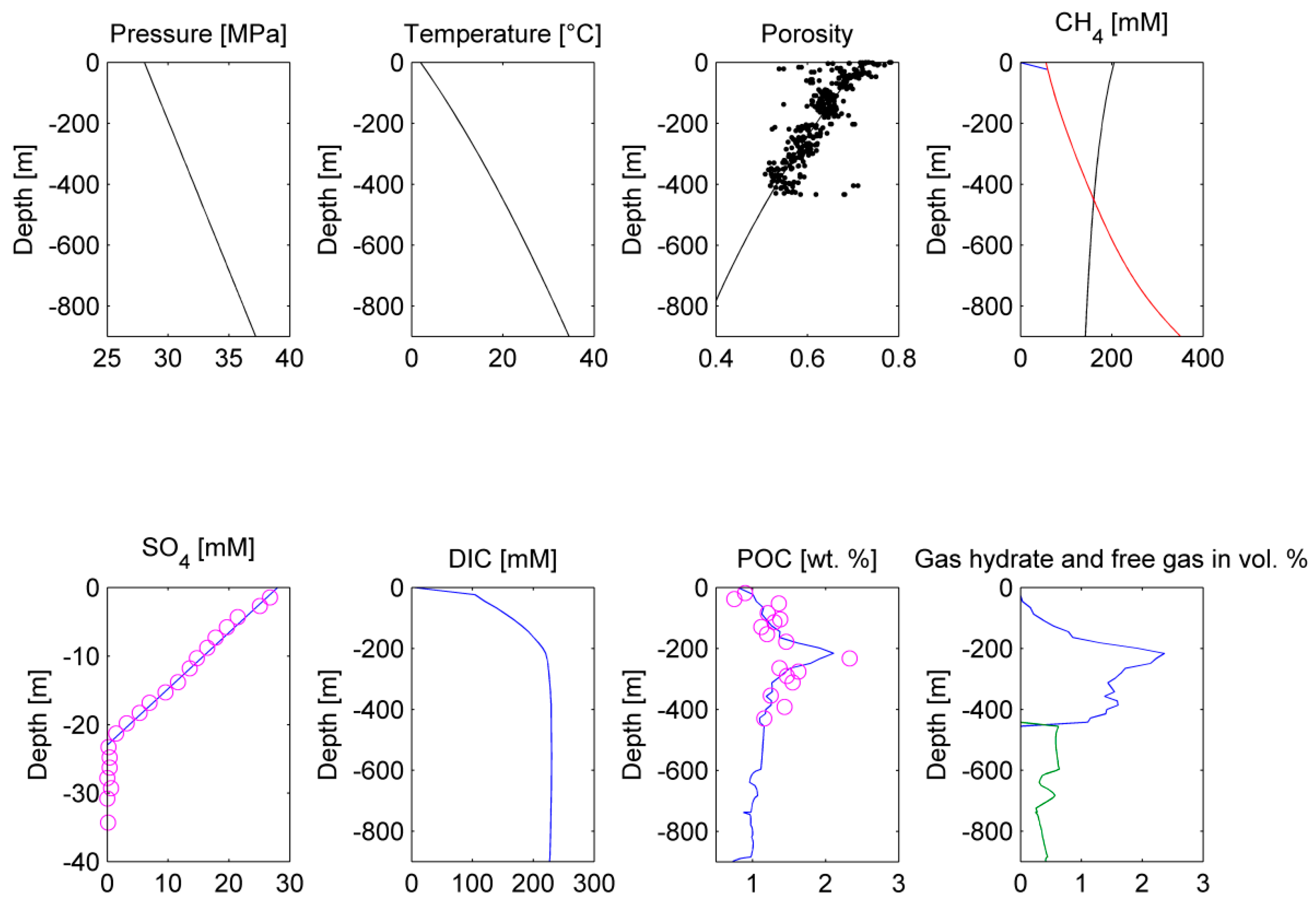
3.3. Scenario 3
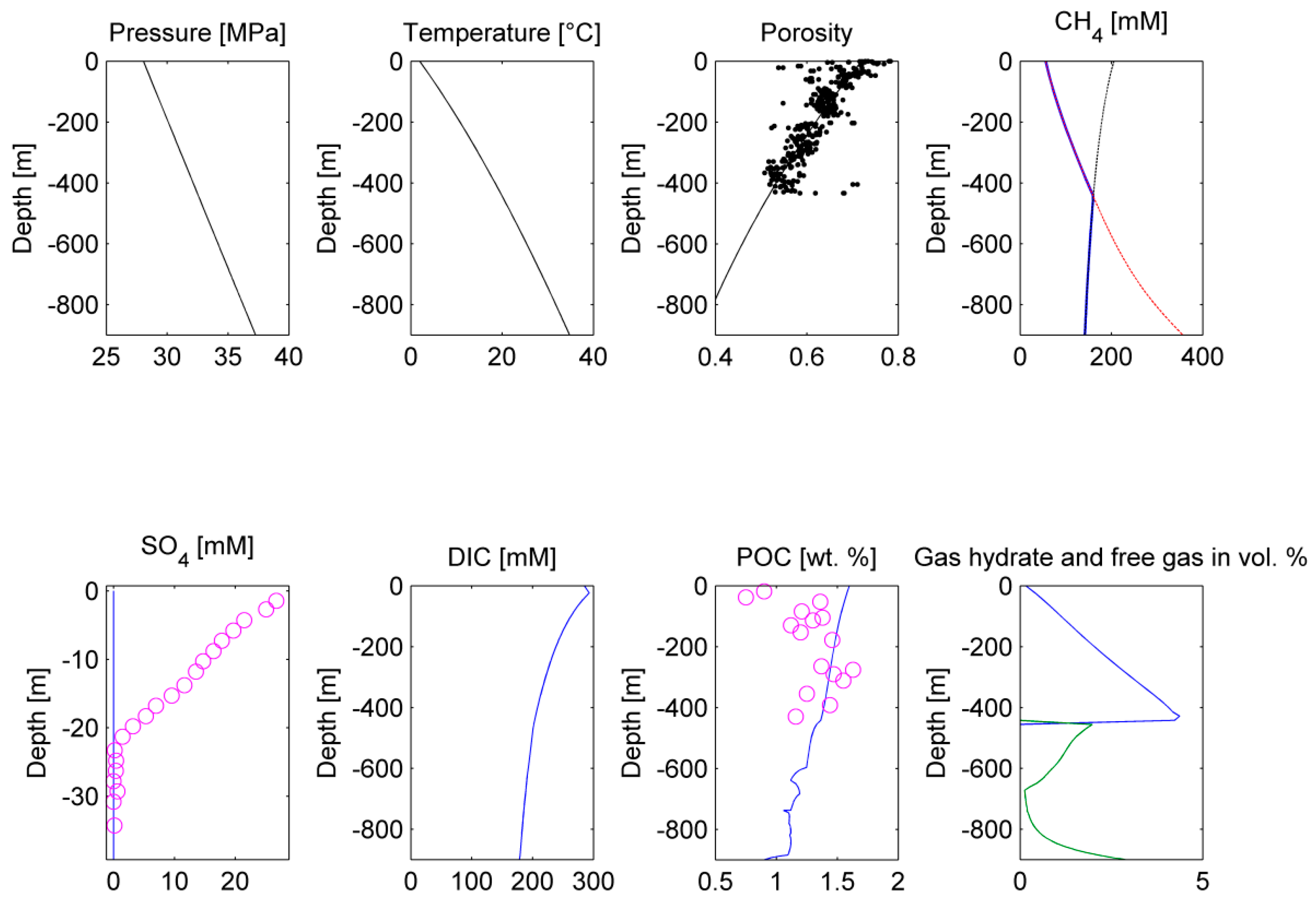
3.4. Scenario 4
3.5. Scenario 5
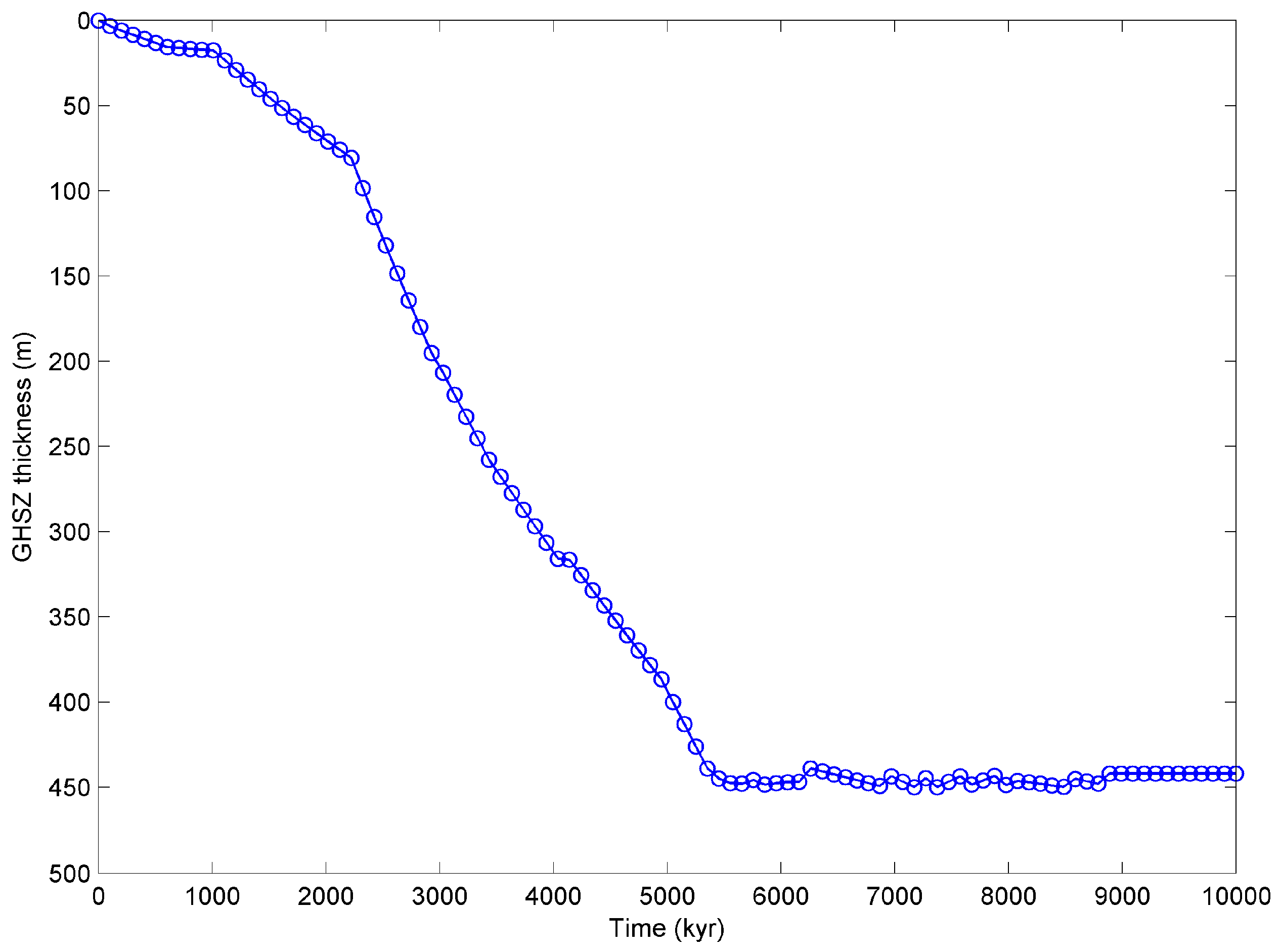
3.6. The Gas Hydrate Stability Zone Base—Evolution in Time
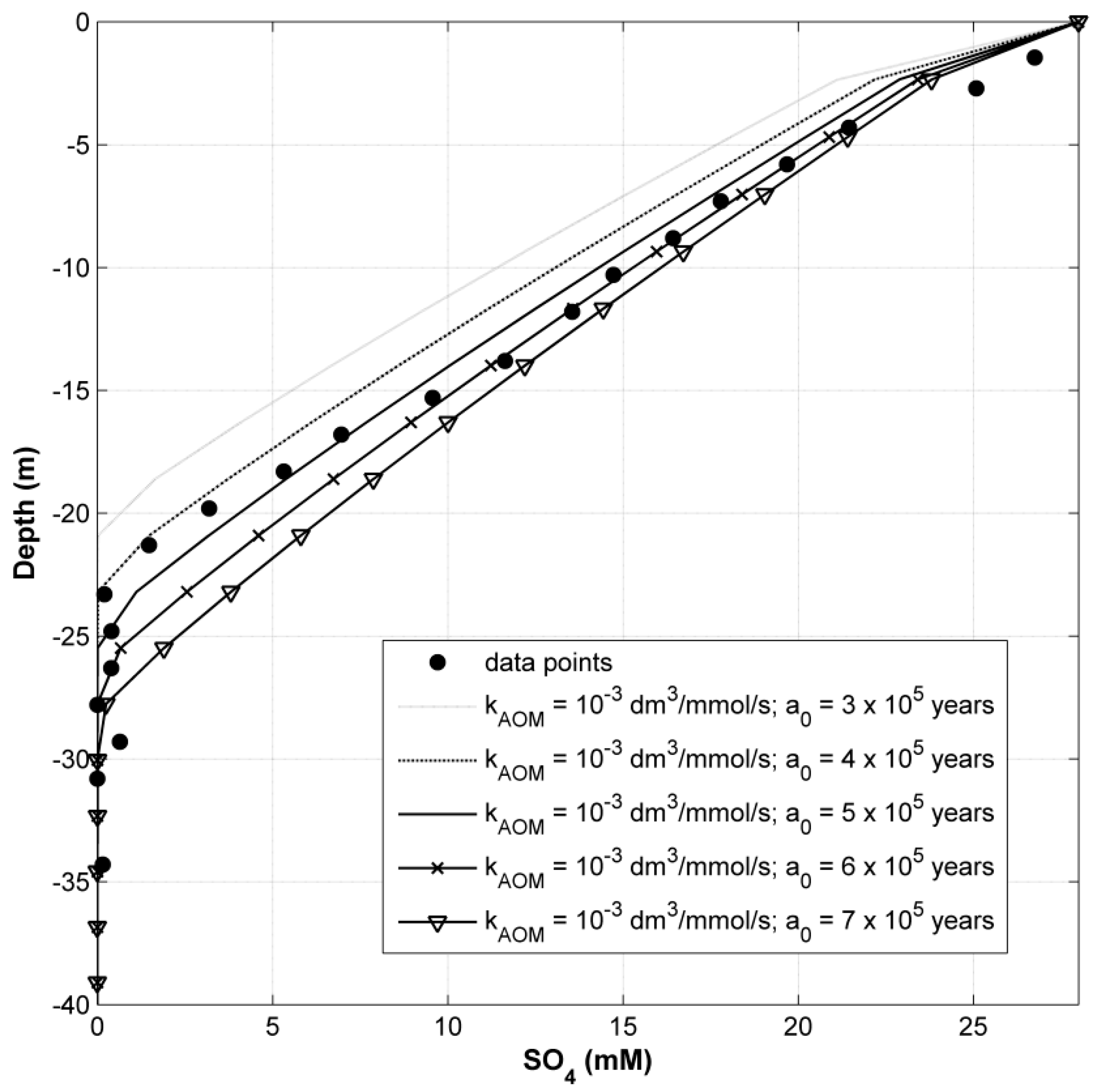
3.7. Model Sensitivity to the Initial Age of Organic Matter Decomposition
4. Conclusions
Author Contributions
Funding
Acknowledgments
Conflicts of Interest
References
- Kretschmer, K.; Biastoch, A.; Ruepke, L.; Burwicz, E. Modeling the fate of methane hydrates under global warming. Glob. Biogeochem. Cycles 2015, 29, 610–625. [Google Scholar] [CrossRef]
- Biastoch, A.; Treude, T.; Rüpke, L.H.; Riebesell, U.; Roth, C.; Burwicz, E.B.; Park, W.; Latif, M.; Böning, C.W.; Madec, G.; et al. Rising Arctic Ocean temperatures cause gas hydrate destabilization and ocean acidification. Geophys. Res. Lett. 2011, 38, 5. [Google Scholar] [CrossRef]
- Phrampus, B.J.; Hornbach, M.J. Recent changes to the Gulf Stream causing widespread gas hydrate destabilization. Nature 2012, 490, 527–530. [Google Scholar] [CrossRef] [PubMed]
- Skarke, A.; Ruppel, C.; Kodis, M.; Brothers, D.; Lobecker, E. Widespread methane leakage from the sea floor on the northern US Atlantic margin. Nat. Geosci. 2014, 7, 657–661. [Google Scholar] [CrossRef]
- Berndt, C.; Feseker, T.; Treude, T.; Krastel, S.; Liebetrau, V.; Niemann, H.; Bertics, V.J.; Dumke, I.; Dünnbier, K.; Ferré, B.; et al. Temporal Constraints on Hydrate-Controlled Methane Seepage off Svalbard. Science 2014, 343, 284–287. [Google Scholar] [CrossRef] [PubMed] [Green Version]
- Hillman, J.I.T.; Burwicz, E.; Zander, T.; Bialas, J.; Klaucke, I.; Feldman, H.; Drexler, T.; Awwiller, D. Investigating a gas hydrate system in apparent disequilibrium in the Danube Fan, Black Sea. Earth Planet. Sci. Lett. 2018, 502, 1–11. [Google Scholar] [CrossRef]
- Minshull, T.A.; Marín-Moreno, H.; Betlem, P.; Bialas, J.; Buenz, S.; Burwicz, E.; Cameselle, A.L.; Cifci, G.; Giustiniani, M.; Hillman, J.I.T.; et al. Hydrate occurrence in Europe: A review of available evidence. Mar. Pet. Geol. 2019. [Google Scholar] [CrossRef]
- Dumke, I.; Burwicz, E.; Berndt, C.; Klaeschen, D.; Feseker, T.; Geissler, W.H.; Sarkar, S. Gas hydrate distribution and hydrocarbon maturation north of the Knipovich Ridge, western Svalbard margin. J. Geophys. Res. Solid Earth 2016, 121, 1405–1424. [Google Scholar] [CrossRef] [Green Version]
- Burwicz, E.; Reichel, T.; Wallmann, K.; Rottke, W.; Haeckel, M.; Hensen, C. 3-D basin-scale reconstruction of natural gas hydrate system of the Green Canyon, Gulf of Mexico. Geochem. Geophys. Geosyst. 2017, 18, 1959–1985. [Google Scholar] [CrossRef] [Green Version]
- Milkov, A.V. Global estimates of hydrate-bound gas in marine sediments: How much is really out there? Earth Sci. Rev. 2004, 66, 183–197. [Google Scholar] [CrossRef]
- Boswell, R.; Collett, T.S. Current perspectives on gas hydrate resources. Energy Environ. Sci. 2011, 4, 1206–1215. [Google Scholar] [CrossRef]
- Burwicz, E.B.; Ruepke, L.H.; Wallmann, K. Estimation of the global amount of submarine gas hydrates formed via microbial methane formation based on numerical reaction-transport modeling and a novel parameterization of Holocene sedimentation. Geochim. Cosmochim. Acta 2011, 75, 4562–4576. [Google Scholar] [CrossRef] [Green Version]
- Buffett, B.; Archer, D. Global inventory of methane clathrate: Sensitivity to changes in the deep ocean. Earth Planet. Sci. Lett. 2004, 227, 185–199. [Google Scholar] [CrossRef]
- Klauda, J.B.; Sandler, S.I. Global Distribution of Methane Hydrate in Ocean Sediment. Energy Fuels 2005, 19, 459–470. [Google Scholar] [CrossRef]
- Dickens, G.R. The potential volume of oceanic methane hydrates with variable external conditions. Org. Geochem. 2001, 32, 1179–1193. [Google Scholar] [CrossRef]
- Wallmann, K.; Piñero, E.; Burwicz, E.; Haeckel, M.; Hensen, C.; Dale, A.W.; Rüpke, L.H. The Global Inventory of Methane Hydrate in Marine Sediments: A Theoretical Approach. Energies 2012, 5, 2449–2498. [Google Scholar] [CrossRef]
- Archer, D.; Buffett, B.; Brovkin, V. Ocean methane hydrates as a slow tipping point in the global carbon cycle. Proc. Natl. Acad. Sci. USA 2009, 106, 20596–20601. [Google Scholar] [CrossRef] [PubMed] [Green Version]
- USGS World Energy Assessment Team. US Geological Survey World Petroleum Assessment 2000—Description and Results; U.S. Geological Survey: Reston, VA, USA, 2000.
- Shipley, T.H.; Houston, M.H.; Buffler, R.T.; Shaub, F.J.; McMillen, K.J.; Ladd, J.W.; Worzel, J.L. Seismic Evidence for Widespread Possible Gas Hydrate Horizons on Continental Slopes and Rises. Aapg Bull. Am. Assoc. Pet. Geol. 1979, 63, 2204–2213. [Google Scholar]
- Paull, C.K.; Matsumoto, R.; Wallace, P.J. 9. Site 997, Shipboard Scientific Party. In Proceeding of the Ocean Drilling Program, Initial Reports; Texas A&M University: College Station, TX, USA, 1996; Volume 164. [Google Scholar]
- Guerin, G.; Goldberg, D.; Melser, A. Characterization of in situ elastic properties of gas hydrate-bearing sediments on the Blake Ridge. J. Geophys. Res. 1999, 104, 17781–17795. [Google Scholar] [CrossRef]
- Paull, C.K.; Matsumoto, R. 1. Leg 164 Overview. In Proceeding of the Ocean Drilling Program, Scientific Results; Texas A&M University: College Station, TX, USA, 2000; Volume 164. [Google Scholar]
- Bunz, S.; Polyanov, S.; Vadakkepuliyambatta, S.; Consolaro, C.; Mienert, J. Active gas venting through hydrate-bearing sediments on the Vestnesa Ridge, offshore W-Svalbard. Mar. Geol. 2012, 332, 189–197. [Google Scholar] [CrossRef]
- Rajan, A.; Mienert, J.; Bunz, S. Acoustic evidence for a gas migration and release system in Arctic glaciated continental margins offshore NW-Svalbard. Mar. Pet. Geol. 2012, 32, 36–49. [Google Scholar] [CrossRef] [Green Version]
- Garg, S.K.; Pritchett, J.W.; Katoh, A.; Baba, K.; Fujii, T. A mathematical model for the formation and dissociation of methane hydrates in the marine environment. J. Geophys. Res. 2008, 113. [Google Scholar] [CrossRef]
- Wallmann, K.; Aloisi, G.; Haeckel, M.; Obzhirov, A.; Pavlova, G.; Tishchenko, P. Kinetics of organic matter degradation, microbial methane generation, and gas hydrate formation in anoxic marine sediments. Geochim. Cosmochim. Acta 2006, 70, 3905–3927. [Google Scholar] [CrossRef]
- Egeberg, P.K.; Dickens, G.R. Thermodynamic and pore water halogen constraints on gas hydrate distribution at ODP Site 997 (Blake Ridge). Chem. Geol. 1999, 153, 53–79. [Google Scholar] [CrossRef]
- Davie, M.K.; Buffett, B.A. A numerical model for the formation of gas hydrate below the seafloor. In Proceedings of the Rock the Foundation Convention, Canadian Society of Petroleum Geologists, Calgary, AB, Canada, 18–22 June 2001. [Google Scholar]
- Xu, W.; Ruppel, C. Predicting the occurence, distribution, and evolution of methane gas hydrate in porous marine sediments. J. Geophys. Res. 1999, 104, 5081–5095. [Google Scholar] [CrossRef]
- Davie, M.K.; Buffett, B.A. Sources of methane for marine gas hydrate: Inferences from a comparison of observations and numerical models. Earth Planet. Sci. Lett. 2003, 206, 51–63. [Google Scholar] [CrossRef]
- Davie, M.K.; Buffett, B.A. A steady-state model for marine hydrate formation: Constraints on methane supply from pore water sulfate profiles. J. Geophys. Res. 2003, 108. [Google Scholar] [CrossRef]
- Claypool, G.E.; Kaplan, I.R. Natural Gases in Marine Sediments; Kaplan, I.R., Ed.; Plenum Press: New York, NY, USA, 1974; Volume 3, pp. 99–139. [Google Scholar]
- Borowski, W.S.; Paull Ch, K.; Ussler, I.I.I.W. Carbon cycling within the upper methanogenic zone of continental rise sediments: An example from the methane-rich sediments overlying the Blake Ridge gas hydrate deposits. Mar. Chem. 1997, 57, 299–311. [Google Scholar] [CrossRef]
- Bryan, G.M. Hydrodynamic model of blake outer ridge. J. Geophys. Res. 1970, 75, 4530–4537. [Google Scholar] [CrossRef]
- Hornbach, M.J.; Saffer, D.M.; Holbrook, W.S. Critically pressured free-gas reservoirs below gas-hydrate provinces. Nature 2004, 427, 142–144. [Google Scholar] [CrossRef]
- Flemings, P.B.; Liu, X.L.; Winters, W.J. Critical pressure and multiphase flow in Blake Ridge gas hydrates. Geology 2003, 31, 1057–1060. [Google Scholar] [CrossRef]
- Ikeda, A.; Okada, H.; Koizumi, I. 35. Data Report: Late Miocene to Pleistocene Diatoms from the Blake Ridge, Site 997. In Proceeding of the Ocean Drilling Program, Scientific Results; Texas A&M University: College Station, TX, USA, 2000; Volume 164. [Google Scholar]
- Paull, C.K.; Lorenson, T.D.; Borowski, W.S.; Ussler, W., III; Olsen, K.; Rodriguez, N.M. 7. Isotopic Composition of CH4, CO2 species, and sedimentary organic matter within samples from the Blake Ridge: Gas source implications. In Proceeding of the Ocean Drilling Program, Scientific Results; Texas A&M University: College Station, TX, USA, 2000; Volume 164. [Google Scholar]
- Dillon, W.P.; Paull, C.K. Natural Gas Hydrates: Properties, Occurrences, and Recovery; Cox, J.L., Ed.; Butterworth: Oxford, UK, 1983; pp. 73–90. [Google Scholar]
- Dickens, G.R.; Paull, C.K.; Wallace, P. Direct measurement of in situ methane quantities in a large gas-hydrate reservoir. Nature 1997, 385, 426–428. [Google Scholar] [CrossRef] [Green Version]
- Hovland, M.; Gallagher, J.W.; Clennell, M.B.; Lekvam, K. Gas hydrate and free gas volumes in marine sediments: Example from the Niger Delta front. Mar. Pet. Geol. 1997, 14, 245–255. [Google Scholar] [CrossRef]
- Ruppel, C. Anomalously cold temperatures observed at the base of the gas hydrate stability zone on the US Atlantic passive margin. Geology 1997, 25, 699–702. [Google Scholar] [CrossRef]
- Davie, M.K.; Buffett, B.A. A numerical model for the formation of gas hydrate below the seafloor. J. Geophys. Res. Solid Earth 2001, 106, 497–514. [Google Scholar] [CrossRef]
- Tishchenko, P.; Hensen Ch Wallmann, K.; Wong, C.S. Calculation of the stability and solubility of methane hydrate in seawater. Chem. Geol. 2005, 219, 37–52. [Google Scholar] [CrossRef]
- Hantschel, T.; Kauerauf, A. Fundamentals of Basin and Petroleum Systems Modeling; Springer: Berlin/Heidelberg, Germany, 2009. [Google Scholar]
- Parker, J.C.; Lenhard, R.J.; Kuppusamy, T. A parametric model for constitutive properties governing multiphase flow in porous media. Water Resour. Res. 1987, 23, 618–624. [Google Scholar] [CrossRef]
- Xu, W.; Germanovich, L.N. Excess pore pressure resulting from methane hydrate dissociation in marine sediments: A theoretical approach. J. Geophys. Res. 2006, 111. [Google Scholar] [CrossRef]
- Friend, D.G.; Ely, J.F.; Ingham, H. Thermophysical properties of methane. J. Phys. Chem. Ref. Data 1989, 18, 583–638. [Google Scholar] [CrossRef]
- Doughty, C. Modeling geologic storage of carbon dioxide: Comparison of non-hysteretic and hysteretic characteristic curves. Energy Convers. Manag. 2007, 48, 1768–1781. [Google Scholar] [CrossRef] [Green Version]
- Manakov, A.Y.; Likhacheva, A.Y.; Potemkin, V.A.; Ogienko, A.G.; Kurnosov, A.V.; Ancharov, A.I. Compressibility of Gas Hydrates. ChemPhysChem 2011, 12, 2475–2483. [Google Scholar] [CrossRef] [PubMed]
- Gabitto, J.F.; Tsouris, C. Physical Properties of Gas Hydrates: A Review. J. Thermodyn. 2010, 2010. [Google Scholar] [CrossRef]
- Rueff, R.M.; Sloan, E.D.; Yesavage, V.F. Heat-capacity and heat of dissociation of methane hydrates. AIChE J. 1988, 34, 1468–1476. [Google Scholar] [CrossRef]
- Boudreau, B.P. Diagenetic Models and Their Implementation: Modelling Transport and Reactions in Aquatic Sediments; Springer: Berlin/Heidelberg, Germany, 1997. [Google Scholar]
- Flogel, S.; Wallmann, K.; Poulsen, C.J.; Zhou, J.; Oschlies, A.; Voigt, S.; Kuhnt, W. Simulating the biogeochemical effects of volcanic CO2 degassing on the oxygen-state of the deep ocean during the Cenomanian/Turonian Anoxic Event (OAE2). Earth Planet. Sci. Lett. 2011, 305, 371–384. [Google Scholar] [CrossRef]
- Middelburg, J.J. A simple rate model for organic matter decomposition in marine sediments. Geochim. Cosmochim. Acta 1989, 53, 1577–1581. [Google Scholar] [CrossRef]
- McDougall, T.J.; Jackett, D.R.; Millero, F.J.; Pawlowicz, R.; Barker, P.M. A global algorithm for estimating Absolute Salinity. Ocean Sci. 2012, 8, 1117–1128. [Google Scholar] [CrossRef]
- Duan, Z.; Moller, N.; Weare, J.H. An equation of state for the CH4-CO2-H2O system: I. Pure systems from 0 to 1000 °C and 0 to 8000 bar. Geochim. Cosmochim. Acta 1992, 56, 2605–2617. [Google Scholar] [CrossRef]
- Deming, D.; Chapman, D.S. Thermal Histories and Hydrocarbon Generation—Example from Utah-Wyoming Thrust Belt. Aapg Bull. Am. Assoc. Pet. Geol. 1989, 73, 1455–1471. [Google Scholar]
- Waite, W.F.; Stern, L.A.; Kirby, S.H.; Winters, W.J.; Mason, D.H. Simultaneous determination of thermal conductivity, thermal diffusivity and specific heat in Si methane hydrate. Geophys. J. Int. 2007, 169, 767–774. [Google Scholar] [CrossRef]
- Schmidt, C.; Burwicz, E.; Hensen, C.; Wallmann, K.; Martinez-Loriente, S.; Gracia, E. Genesis of mud volcano fluids in the Gulf of Cadiz using a novel basin-scale model approach. Geochim. Cosmochim. Acta 2018, 243, 186–204. [Google Scholar] [CrossRef]
- Karstens, J.; Haflidason, H.; Becker, L.W.M.; Berndt, C.; Rüpke, L.; Planke, S.; Liebetrau, V.; Schmidt, M.; Mienert, J. Glacigenic sedimentation pulses triggered post-glacial gas hydrate dissociation. Nat. Commun. 2018, 9, 11. [Google Scholar] [CrossRef] [PubMed]


| Parameter | Value | References |
|---|---|---|
| Water depth | 2781 m | [20,33] |
| Bottom water temperature | 3.4 °C | [20] |
| Geothermal gradient | 0.035 °C·m−1 | [20] |
| Salinity | 35 PSU | [20] |
| Gas composition | 99% CH4, 1% CO2 (here assumed 100% CH4) | [38] |
| Seafloor porosity | 0.7 | Curve fitting parameter |
| Compaction length scale | 0.75 × 10⁻³ m−1 | Curve fitting parameter |
| Organic carbon available at the seafloor | 1.6 wt.% | [20,33] |
| Epoch | Age (Ma) | Value (mm∙yr−1) | Sediment Depth after Compaction (mbsf) |
|---|---|---|---|
| Pleistocene | 0–0.53 | 0.235 | 0–18 |
| 0.53–1.26 | 0.105 | 18–48 | |
| 1.26–1.65 | 0.220 | 48–70 | |
| Pliocene | 1.65–2.51 | 0.140 | 70–110 |
| 2.51–2.55 | 0.010 | 110–118 | |
| 2.55–2.76 | 0.145 | 118–151 | |
| 2.76–3.62 | 0.180 | 151–308 | |
| 3.62–3.72 | 0.155 | 308–324 | |
| 3.72–4.43 | 0.205 | 324–339 | |
| 4.43–4.97 | 0.055 | 339–415 | |
| Late Miocene | 4.97–5.59 | ~0.060 | 415–552 |
| 5.59–5.92 | ~0.005 | 552–588 | |
| 5.92–6.6 | ~0.025 | 588–750 |
| Parameter | Symbol | Value | References |
|---|---|---|---|
| Gravitational acceleration | g | 9.81 m∙s−2 | - |
| Density of sediment grains | ρs | 2650 kg∙m3 | - |
| Density of gas hydrate | ρh | 913 kg∙m3 | - |
| Intrinsic permeability | k | Equation (7) | [45] |
| Geometrical factor | B | 0.5 | [45] |
| Specific surface area | S | 107 m2/m3 | [45] |
| Relative permeability of fluid | krf | Equation (8) | [46] |
| Relative permeability of gas | krg | Equation (9) | [46] |
| Dynamic viscosity of fluid | μf | 10−3 Pa∙s | [47] |
| Dynamic viscosity of gas | μg | 11.5 × 10⁻⁶ Pa∙s | [48] |
| Sediment factor | m | 0.197 | [49] |
| Residual water saturation | Srf | 0.03 | [49] |
| Residual gas saturation | Srg | 0.05−0.1 | This study |
| Compressibility of fluid | βf | 4 × 10⁻¹⁰ Pa−1 | [45] |
| Compressibility of gas | βg | 10−7 Pa−1 | [45] |
| Compressibility of hydrate | βh | 10−15 Pa−1 | [50] |
| Thermal conductivity of solids | λs | 2.4 W∙m−1∙K−1 | [45] |
| Thermal conductivity of fluid | λf | 0.6 W∙m−1∙K−1 | [45] |
| Thermal conductivity of gas | λg | 1 W∙m−1∙K−1 | [45] |
| Thermal conductivity of hydrate | λh | 0.50 W∙m−1∙K−1 | [51] |
| Specific heat capacity of solids | Cps | 835 J∙kg−1∙K−1 | [45] |
| Specific heat capacity of fluid | Cpf | 4181.3 J∙kg−1∙K−1 | [45] |
| Specific heat capacity of gas | Cpg | 2200 J∙kg−1∙K−1 | [45] |
| Specific heat capacity of hydrate | Cph | 1650 J∙kg−1∙K−1 | [52] |
| Parameter | Symbol | Value | References |
|---|---|---|---|
| Initial age of organic matter decomposition | a0 | 5 × 10⁵ years | [26] |
| Monod inhibition constant of organic matter degradation by DIC and CH4 | Kc | 40 mM | [26] |
| Monod inhibition constant of CH4 formation by SO4 | KSO4 | 1 mM | [26] |
| Kinetic constant for AOM | kAOM | 1 cm3∙year−1∙mmol−1 | [26] |
| Sulfate concentration at the upper model boundary | CSO4 | 28 mM | [20] |
| Methane concentration at the upper boundary | CCH4 | 10−4 mM | [26] |
| Dissolved Inorganic Carbon (DIC) concentration at the upper boundary | CDIC | 4 mM | [26] |
© 2019 by the authors. Licensee MDPI, Basel, Switzerland. This article is an open access article distributed under the terms and conditions of the Creative Commons Attribution (CC BY) license (http://creativecommons.org/licenses/by/4.0/).
Share and Cite
Burwicz, E.; Rüpke, L. Thermal State of the Blake Ridge Gas Hydrate Stability Zone (GHSZ)—Insights on Gas Hydrate Dynamics from a New Multi-Phase Numerical Model. Energies 2019, 12, 3403. https://doi.org/10.3390/en12173403
Burwicz E, Rüpke L. Thermal State of the Blake Ridge Gas Hydrate Stability Zone (GHSZ)—Insights on Gas Hydrate Dynamics from a New Multi-Phase Numerical Model. Energies. 2019; 12(17):3403. https://doi.org/10.3390/en12173403
Chicago/Turabian StyleBurwicz, Ewa, and Lars Rüpke. 2019. "Thermal State of the Blake Ridge Gas Hydrate Stability Zone (GHSZ)—Insights on Gas Hydrate Dynamics from a New Multi-Phase Numerical Model" Energies 12, no. 17: 3403. https://doi.org/10.3390/en12173403