Multi-Objective Optimization of Off-Grid Hybrid Renewable Energy Systems in Buildings with Prior Design-Variable Screening

Abstract

This work presents an optimization strategy and the cost-optimal design of an off-grid building served by an energy system involving solar technologies, thermal and electrochemical storages. Independently from the multi-objective method (e.g., utility function) and algorithm used (e.g., genetic algorithms), the optimization of this kind of systems is typically characterized by a high-dimensional variables space, computational effort and results uncertainty (e.g., local minimum solutions). Instead of focusing on advanced optimization tools to handle the design problem, the dimension of the full problem has been reduced, only considering the design variables with a high “effect” on the objective functions. An off-grid accommodation building is presented as test case: the original six-variable design problem consisting of about 300,000 possible configurations is reduced to a two-variable problem, after the analysis of 870 Monte Carlo simulations. The new problem includes only 220 possible design alternatives with a clear benefit for the multi-objective optimization algorithm. The energy-economy Pareto frontiers obtained by the original and the reduced problems overlap, showing the validity of the proposed methodology. The No-RES (no renewable energy sources) primary energy consumption can be reduced up to almost 0 kWh/(m²yr) and the net present value (NPV) after 20 years can reach 70 k€ depending on the number of photovoltaic panels and electrochemical storage size. The reduction of the problem also allows for a plain analysis of the results and the drawing of handy decision charts to help the investor/designer in finding the best design according to the specific investment availability and target performances. The configurations on the Pareto frontier are characterized by a notable electrical overproduction and a ratio between the two main design variables that goes from 4 to 8 h. A sensitivity analysis to the unitary price of the electrochemical storage reveals the robustness of the sizing criterion.

1. Introduction

Planning in the medium-long term the construction of an integrated thermal and electrical energy production system fed by renewable sources (also known as hybrid renewable energy systems, HRES) is certainly a tricky but interesting investment decision that occurs under multiple uncertainties. In recent years, in fact, the deregulation of the electricity sector, as well as the introduction of environmental constraints, has significantly stimulated the market of solutions for local energy production and consequently raised the attention of investors to new business opportunities, also adding new variables and constraints that further complicate the investment decision [1]. As an example, one can cite the call for reduction of greenhouse gas emissions, the new targets for penetration of renewable energy sources (RES) in the electricity generating mix (Directive 2009/28/EC) and the Energy Performance of Buildings Directives (2010/31/EU and 2018/844/EU), which require new buildings to be nearly zero-energy by the end of 2020.

In this context, energy capacity planning and optimal power generation mix (or portfolio) are among the most challenging and investigated topics, both in a large-scale perspective, as for the national electricity generation system [2], and for small-scale plants, as stand-alone configurations or autonomous buildings [3,4,5]. Critical issues typically addressed are: the number of different energy sources to be included into the HRES; the type of technology of the generation sub-systems (conventional or not); the design parameters of the HRES (size, control, and management policies); the strategies used for decision assessment.

Many possible system configurations and uncertain variables should be considered in the problem formulation [6,7,8,9,10]. Furthermore, the increased complexity of HRES with respect to the systems fed by a single form of energy is due to the non-linear characteristics of the components, the high number of variables and parameters that have to be considered for the optimal design, and the fact that the ideal configuration and the optimal control strategy are interdependent [11]. Modern HRES are generally integrated (electrical, thermal components and buildings), made of highly-coupled subsystems where different technologies (e.g., renewable energy systems and traditional generators) cooperate for concurrent multiple objectives, such as reliability, cost efficiency, environmental sustainability, indoor comfort, and indoor air quality [12]. This condition calls for a robust and more integrated approach to the evaluation of the best system design, able to deal with the increasing complexity of the decision context, an accurate but efficient dynamic modeling of components interconnections, and decision tools able to address the stakeholders towards the most efficient and cost-effective solutions [13,14,15].

In [11,16,17,18] the authors presented a significant review of studies regarding stand-alone HRES. Evidence shows a great variety of design, simulation, control and optimization approaches, as well as available software, such as HOMER (Hybrid Optimization Model for Electric Renewables, HOMER Energy, Boulder, CO, USA), the most used tool for electric energy systems, developed by NREL (National Renewable Energy Laboratory, Golden, CO, USA). Indeed, concerning the design and simulation of HRES, most of the works focus on the sole electricity generation, while many thermal aspects and the model of the building are often oversimplified or neglected. Faccio et al. Reference [19] presented an interesting review of the most recent works on the optimal design of HRES. The cost factor is the most common optimization goal, together with environmental emissions. Only in a few cases do the works aim to optimize the operation of a specific, most delicate component (e.g., the electric battery). In [20], the authors reviewed the main methodologies used for the optimization, highlighting positive aspects and drawbacks of each modeling technique, such as linear programming, particle swarm optimization, Monte Carlo analyses, and hybrid techniques.

The large number of research works in this field shows that HRES are a topic of great interest, in particular because highly interacting energy systems cannot be analyzed by traditional design approaches. However, to the best of our knowledge, universal straightforward design procedures and decision criteria do not exist, as any specific project has peculiar characteristics, objectives and priorities set by the decision maker. The multi-objective optimal design requires the set-up of a multi-variable optimization problem with all the well-known drawbacks, such as computational effort, selection of the multi-objective method, optimization algorithms, physical interpretation, uncertainty and robustness of the resulting optimal configurations.

Recent reviews on optimization techniques applied in HRES design [21,22,23] present a general trend in analyzing, classifying and developing novel algorithms according to their ability to handle high-dimension variable spaces [24]. On the contrary, there is a limited attention on the potential of the preliminary analysis of the design space, to determine which variables are the main drivers of system performances and consequentially reduce the dimension of the problem. The latter approach is well-known in the design-of-experiments technique with the name of “factors screening” [25], in which the number of experiment variables (i.e., the factors) is limited for practical and economic reasons. A similar approach can be used in the multi-variable optimization problems [26], to reduce the design space, use simpler optimization techniques, but preserving the quality of the final solution.

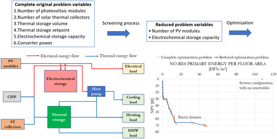
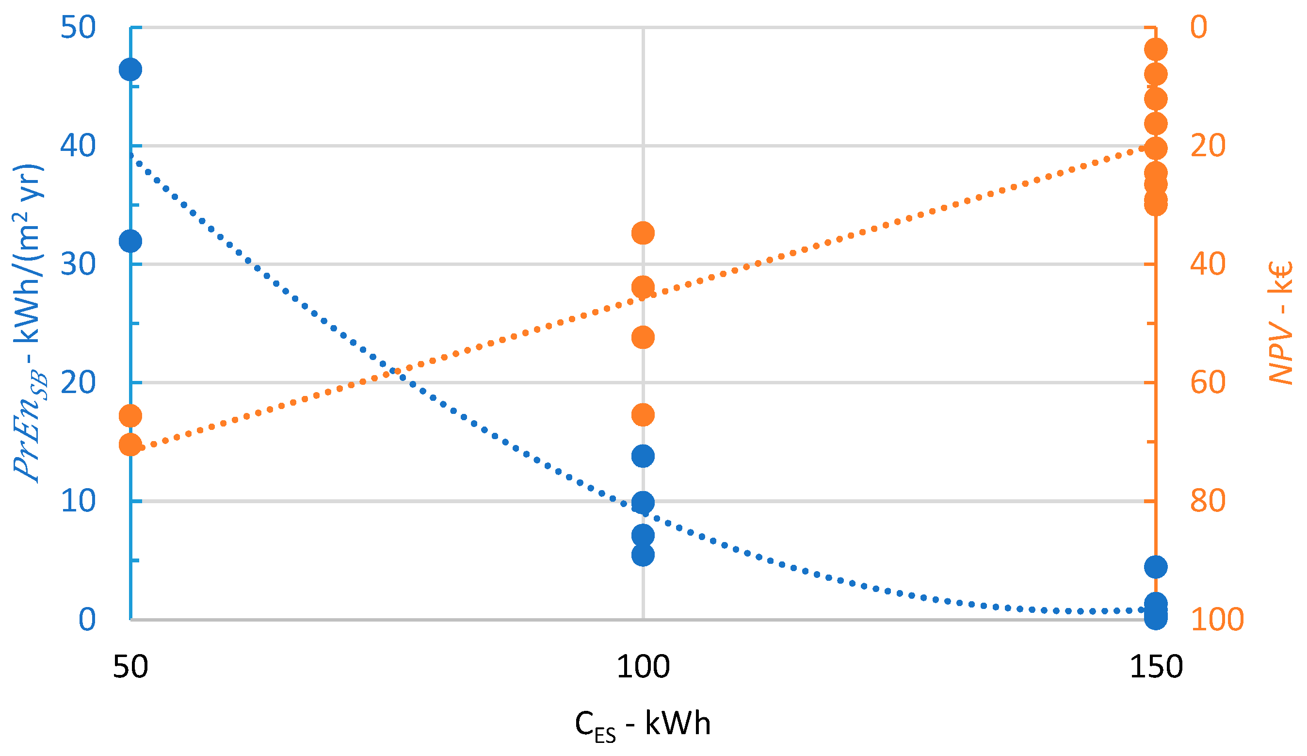
This work applies this approach to the multi-objective optimization of a HRES system, showing the advantages at the computational level, but also (and particularly) in terms of engineering understanding of the problem, interpretation of results, and support for the decision maker in the investment analysis and HRES planning. The work includes:

• An integrated model for the simulation of the HRES and the building dynamics based on holistic and validated physical models to assess both thermal and electrical energy flows during the system lifetime, with low computational requirements. The strength of this approach is that, conversely to the aforementioned scientific literature, it considers the proper size and operation of each single component in the perspective of the global performance of the entire system, both for electrical and thermal aspects. The main drawback consists of the accuracy of the subsystem models, which must be coherent with the simulation time step and the uncertainty of the energy fluxes estimation;
• A multi-objective optimization procedure that considers the targets of environmental sustainability together with the traditional financial performance of investments;
• A screening methodology aimed at reducing the computational effort of the multi-objective algorithm. The optimization procedure is limited only to those variables with a high correlation (or “effect”) with the objective functions. The total computational effort of the variable identification and reduced optimization problem is very low with respect to the original problem. Together with the computational effort, a reduced optimization problem has the following advantages:

  ○

  an easier interpretation of the optimal design(s) found by the optimization algorithm, such as operative features of the system and possible correlations among the optimal value of the main design variables;

  ○

  the drawing of handy decision charts that can be used by the decision makers to assess the energy and economic performance of the design alternatives, helping the selection of the best configurations according to the specific objectives and priorities;

  ○

  a simpler sensitivity analysis to investigate the robustness of the optimal solutions identified by the sizing procedure.

The presented case study is representative of an autonomous small-to-medium accommodation building (off-grid, both electricity and gas) in mild-Mediterranean climates; anyway, the proposed approach is generic enough to be applied also to any energy system optimization, both for stand-alone and on-grid building-integrated HRES.

This paper is organized as follows: Section 2 describes the reference HRES system and the energy and economy modelling methods. Section 3 illustrates the reduction methodology based on a random sample correlation analysis. The results, the post-processing analysis, and the related discussion are presented in Section 4. Section 5 presents the sensitivity analysis, and conclusions are finally provided in Section 6.

2. Hybrid Renewable Energy Systems (HRES) Energy and Economy Modelling

In this work, we refer to the optimal design of an off-grid building served by a HRES system, according to cost-benefit considerations. The reference facility is an off-grid small-to-medium accommodation building, located in an isolated area of the countryside in a mild-Mediterranean region. Energy requirements include heating, cooling, domestic hot water (DHW), and electrical services. To address these loads, an integrated system including solar thermal panels, photovoltaic modules, thermal storage (TS), electrochemical storage (ES), a heat pump (HP), and a combined heat and power system (CHP) must be optimally designed. A schematic representation of the overall system is presented in Figure 1.

As the building is a stand-alone one, particular attention should be given in the design of the overall HRES system, as all the technologies have to be designed and integrated to address the building requirements, without oversizing, so avoiding additional costs and, in some cases, also worse operating performances (e.g., heat pumps). The overall building and energy system are analyzed through an hourly dynamic simulation, using literature or in-house mathematical models shortly discussed in Section 2.1, Section 2.2, Section 2.3 and Section 2.4.

2.1. External Climate and Building Envelope Model

The hourly heating and cooling loads, $E_{th,H}$ and $E_{th,C}$, are evaluated correlating the design thermal load and a mean external temperature ${\overline{T}}_{ext}$ on the effective time shift of the building [27,28]. For the summer season, the mean sol-air temperature [28,29] on the same time shift of the building, ${\overline{T}}^{*}{}_{ext}$, is considered, instead of the external temperature. The two equations read:

$$E_{th,H}=P_H\left(1-\frac{{\overline{T}}_{ext}-T_{des,H}}{T_{off,H}-T_{des,H}}\right)$$

(1a)

$$E_{th,C}=P_C\left(1-\frac{{\overline{T}}^{*}{}_{ext}-T_{des,C}^{*}}{T_{off,C}-T_{des,C}^{*}}\right)$$

(1b)

Typical hotel schedules are used as DHW and electrical load profiles, including induction cooking, lighting, and household appliances [30]. Further details about the characterization of the energy requirements profiles can be found in [31].

2.2. Modeling of the Generation System

The performance of the photovoltaic (PV) modules are evaluated through the assessment of the cell temperature, depending on the clearness of the sky $K_t$ [32] and the external temperature, $T_{ext}$, using the model discussed in [33]. The equations read:

$$T_{PV}=T_{ext}+\left(219+832K_t\right)\frac{NOC{T}_{PV}-20}{800}$$

(2a)

$${\eta }_{PV}={\eta }_{inv}\left({\eta }_{PV,ref}\left[1-{\beta }_{T,PV }\left(T_{PV}-T_{ref,PV}\right)\right]\right)$$

(2b)

$$E_{PV}={\eta }_{PV}{S}_{PV}{I}_{sol}$$

(2c)

As for the evaluation of the solar thermal system (ST) panels’ efficiency, classical models in literature and technical standards are used [32,34]. The Equations read:

$${\eta }_{ST}=F_R{\left(\tau \alpha \right)}_n\left(1-b_0\left(\frac{1}{\cos \theta }-1\right)\right)-\frac{F_R{U}_L\left(T_{ST,in}-T_{ext}\right)}{I_{sol}}$$

(3a)

$$E_{ST}={\eta }_{ST}{S}_{ST}{I}_{sol}$$

(3b)

where $T_{ST,in}$ is assumed equal to the water temperature in the thermal storage (see Equation (5)).

The heat pump is a pivotal element in the system, as it links thermal and electrical energy fluxes. It can receive electrical energy from the PV modules, the CHP generator, or the electrochemical storage and provide energy to: (i) the cooling service directly to the building; (ii) for the heating service, either directly to the building or through the thermal storage, and (iii) for the DHW service, heating the thermal storage. On the contrary, the ST collectors can only provide thermal energy to the thermal storage. The heat pump performances are evaluated through the second-law efficiency method [35], using a fixed value of both ${\eta }_H^{II}$ and ${\eta }_C^{II}$ (assessed through manufacturers’ data), the outdoor temperature, $T_{ext}$, and the supply water temperature $T_{cond}$/$T_{eva}$ for the evaluation of the ideal COP/EER. The equations read:

$$COP={\eta }_H^{II}CO{P}_{id}={\eta }_H^{II}\frac{T_{cond}}{T_{cond}-T_{ext}}$$

(4a)

$$EER={\eta }_C^{II}EE{R}_{id}={\eta }_C^{II}\frac{T_{eva}}{T_{ext}-T_{eva}}$$

(4b)

The CHP consists of a diesel-engine generator. When necessary, it recharges the electrochemical storage to the assumed minimum state of charge and/or delivers the electrical load that cannot be provided by the ES due to the power limits of the converter. Fixed values for the electrical power generation efficiency, ${\eta }_{CHP,el}$, and thermal power recovery efficiency,${\eta }_{CHP,th}$, are used.

2.3. Modeling of the Thermal Storage

A simplified lumped-element thermal storage model is considered to evaluate the $T_{TS}$ evolution considering heat inputs (thermal energy from the CHP, solar thermal collectors, heat pump, and recovered energy from PV overproduction), heat outputs (energy used for heating and DHW services), thermal losses, and the variation of internal energy. The equations read:

$$V_{TS}{\rho }_w{c}_w\left(T_{TS}^{t+1}-T_{TS}^t)\right)=E_{CHP,th}^t+E_{ST}^t+E_{HP,TS}^t+E_{PV,oprd}{\eta }_{rec}-\left(E_{TS,H }^t+E_{TS,DHW}^t\right)-E_{TS,l}^t$$

(5a)

$$E_{TS,l }^t=S_{TS}\frac{{\lambda }_{TS}}{s_{TS}}\left(T_{TS}^t-T_{ext,TS}^t\right)$$

(5b)

The thermal storage is kept at a temperature equal or higher than the set-point temperature $T_{TS,set}$ by the thermal generators. When its temperature is higher than the threshold value $T_{TS,UP }$, the heat pump is switched-off from direct heating mode and the heating service is provided by the thermal storage.

2.4. Modeling of the Electrochemical Storage

During standard plant operation, the electrochemical storage receives the surplus of the energy produced by the PV systems and/or delivers the load deficit that cannot be met by the PV. Lithium technology has been taken as reference. In fact, despite the relative high costs with respect to less expensive technologies (i.e., lead-acid batteries, etc.), in the last few years lithium batteries have been considered increasingly also for stationary applications, for their better performance in cycle-life. In fact, being able to sustain from tens up to hundreds of charging-discharging cycles, they can require a very short number (or none) of substitutions during the useful life of the considered application, thus becoming preferable to the previous technologies.

The operative state of charge is assumed to be between the 10% and the 90% of the nominal energy, $E_{ES,nom}$. About storage losses, a constant round trip efficiency, ${\eta }_{\mathrm{ES}}$, is supposed, as usual in literature. The state of charge $So{C}_{\mathrm{ES}}^t$, i.e., the ratio between the charge stored inside and the battery capacity (extractable charge) at a reference current and temperature, is evaluated at any time step as follows:

$$So{C}_{ES}^{t+1}=\min \left\{0.9{\overline{E}}_{ES,nom} ;\max \left[0.1E_{ES,nom} ;So{C}_{ES}^t+\Delta So{C}_{ES}^t\right]\right\}$$

(6a)

$$\Delta So{C}_{ES}^t=\min \left[{\eta }_{ES}{E}_{el,oprd}^t;P_{ES}\right]-\min \left[E_{el,def}^t/{\eta }_{ES};P_{ES}\right]$$

(6b)

$$E_{el,oprd}^t=\max \left[0;E_{PV}^t-\frac{E_{th,H}^t}{CO{P}_H^t}-\frac{E_{th,C}^t}{EE{R}^t}-\frac{E_{HP,TS}^t}{CO{P}_{TS}^t}-E_{OU}^t\right]$$

(6c)

$$E_{el,def}^t=\max \left[0;\frac{E_{th,H}^t}{CO{P}_H^t}+\frac{E_{th,C}^t}{EE{R}^t}+\frac{E_{HP,TS}^t}{CO{P}_{TS}^t}+E_{OU}^t-E_{PV}^t\right]$$

(6d)

Possible overloads are assumed to be dissipated, while the CHP unit provides the electrical energy to keep the $So{C}_{ES}$ at least at $0.1 E_{ES,nom}$ at any time. Besides, the CHP meets the remaining electrical load when the demand is higher than the maximum capacity of the converter.

With regard to the storage lifetime, it must be carefully verified if the considered usage of electrochemical storage at many charging-discharging cycles could rise concerns about its life. Thus, considering experimental data reported in literature [36,37,38] and from manufacturers’ indications [39], and focusing the attention, as said, on lithium technology, an electrochemical storage subject to such solicitation can follow the behavior as depicted in Figure 2. Different typologies are typically available in the general category of lithium batteries, depending on the electrode typology (e.g., LFP, lithium iron phosphate, NMC, nickel manganese cobalt, etc.). From the presented test data, the average trend, calculated as arithmetic mean of the different allowed charging-discharging cycles at the same abscissa, has also been reported in Figure 2, in orange color. As shown, in the case of shallow charging-discharging cycles, battery life expectation can reach hundreds of thousands of micro-cycles, while just few thousands are sustainable when extended depth of discharge is considered. These results have been used to evaluate the battery allowed number of cycles, in order to finalize the economy analysis in Section 2.5. In particular, the black curve of the “worst” case among the examined technologies has been considered as precautionary measure. The latter curve has been discretized in a five-step piecewise function as shown in

Table 1. Maximum number of charging-discharging cycles, $\#cycle@EO{L}_l$, depending on the depth of discharge level, $\Delta So{C}_{ES}/{\overline{E}}_{ES,nom}$.

$\mathit{l}\text{-}\mathbf{th}\mathit{S}\mathit{o}{\mathit{C}}_{\mathit{E}\mathit{S}}\mathbf{Bin}$	$\mathit{\Delta }\mathit{S}\mathit{o}{\mathit{C}}_{\mathit{E}\mathit{S}}/{\mathit{E}}_{\mathit{E}\mathit{S},\mathit{n}\mathit{o}\mathit{m}}$	$\#\mathit{c}\mathit{y}\mathit{c}\mathit{l}\mathit{e}@\mathit{E}\mathit{O}{\mathit{L}}_{\mathit{l}}$
1	0.74–0.90	800
2	0.58–0.74	1000
3	0.42–0.58	3000
4	0.26–0.42	8000
5	0.1–0.26	40,000

.

The number of cycles in each bin is evaluated according to the depth of discharge (DOD), i.e., the ratio between the extracted charge and the battery capacity (extractable charge) at a reference current and temperature, of each charging–discharging cycle occurring during the system lifetime. Due the reduced power typically delivered in building systems (see Section 4.2), C-rate, i.e., the amplitude of the current solicitation, expressed as multiples of the battery capacity, and temperature are assumed to stay around their nominal values. Therefore, for simplicity, dependency from C-rate and temperature was not included in Equation (7), which only considers DOD. For instance, the counter $\#cycl{e}_1$ is the number of cycles with a relative depth of discharge $\Delta So{C}_{ES}/E_{ES,nom}$ between 0.9 and 0.74, $\#cycl{e}_2$ is the number of cycles with a relative depth of discharge $\Delta So{C}_{ES}/E_{ES,nom}$ between 0.74 and 0.58, and so on. The cumulative damage of the ES at the t-th time step is evaluated through Equation (7). When ${\mathrm{ES}}_{dam}^t\ge 1$, the electrochemical storage is substituted and all the counters are reset to zero.

$$E{S}_{dam}^t={\displaystyle \sum }_{i=1}^t{\displaystyle \sum }_{l=1}^5\#cycl{e}_l^t/\#cycle@EO{L}_l$$

(7)

2.5. Economic Analysis

The net present value (NPV) is assumed as the main economic indicator. For the j-th system configuration, the NPV is calculated comparing the actual cash flow with the option of not investing in a HRES, but using a CHP to meet both electrical and thermal energy demands (i.e., No-RES or no renewable energy sources configuration).

$$NPV=T{C}_{No-RES}^N-T{C}_j^N$$

(8)

$$T{C}_j^t={\tilde{C}}_j^0+{\displaystyle \sum }_i^t\left[\frac{{\tilde{C}}_{rpl,j}^i+{\tilde{C}}_{O\&M,j}^i-{\delta }_{t=N}{P}_{shs,j}}{{\left(1+R_d\right)}^i}\right]$$

(9)

The total cost at the t-th year, $T{C}_j^t$, is given by the total initial installation cost, ${\tilde{C}}_j^0$, the operation and maintenance ($O\&M$) costs, ${\tilde{C}}_{O\&M,j}^i$ (which includes the fuel costs), the replacement cost of the devices that have exhausted their operational life, ${\tilde{C}}_{rpl,j}^i$, the positive cash flows due to the possible residual value, $P_{shs,j}$, of the components after the whole system lifetime. In other words, the Boolean variable ${\delta }_{t=N}$ in Equation (9) is equal to 1 only in the N-th year.

The initial cost for the j-th configuration is given by the sum of the installation cost of each component, namely:

$${\tilde{C}}_j^0={\tilde{c}}_{PV}^0{n}_{PV,j}+{\tilde{c}}_{ST}^0{n}_{ST,j}+{\tilde{c}}_{TS}^0{V}_{TS,j}+{\tilde{c}}_{ES}^0{E}_{ES,nom, j}+{\tilde{c}}_{P_{ES}}^0{P}_{ES,j}+{\tilde{C}}_{CHP,j}^0+{\tilde{C}}_{HP}^0$$

(10)

where ${\tilde{c}}_{PV}^0$, ${\tilde{c}}_{ST}^0$, ${\tilde{c}}_{TS}^0$, ${\tilde{c}}_{ES}^0$, ${\tilde{c}}_{P_{ES}}^0$ are the unitary costs of the photovoltaic modules, solar thermal collectors, thermal storage, electrochemical storage, and electrochemical storage converter, respectively. The heat pump capacity is assumed as constant for all the tested configuration as its value only depends on the heating and cooling design load of the building. The CHP sizing and installation cost depends on the maximum electrical power output required in the j-th configuration during the year and it is thus related to the number of PV modules and the electrochemical storage and converter capacities. However, a minimum back-up power of 2.5 kW_el is always installed, namely:

$${\tilde{C}}_{CHP,j}^0={\tilde{c}}_{CHP}^0\max \left[P_{CHP,el,j}^t ;2.5\right]$$

(11)

The operation and maintenance costs are distinguished into variable costs, proportional to the energy use (i.e., the CHP fuel costs) and fixed costs, which include annual assurance costs, programmed maintenance, etc. The latter is assumed proportional to the PV capacity, so the yearly $O\&M$ cost is equal to:

$${\tilde{C}}_{O\&M,j}^t={\tilde{c}}_{f,CHP}{E}_{CHP,in,j}+{\tilde{c}}_{O\&M}{S}_{PV}{n}_{PV,j}/S_{PV,kW}$$

(12)

The replacement cost, ${\tilde{C}}_{rpl,j}^i$, is the present value of the initial installation cost of the replaced sub-system. The main assumption under this hypothesis is that the adopted technologies are similar over the years, so they only experience a price variation in line with the assumed inflation rate, but they do not change their performance or operational duration. In this study, the electrochemical storage and the CHP generator are the only components that need to be replaced during the HRES lifetime. The replacement years for both subsystems are evaluated according to Equation (14), thus accounting for the simulated operational conditions and time.

$${\tilde{C}}_{rpl,j}^t={\tilde{C}}_{ES,rpl,j}^t+{\tilde{C}}_{CHP,rpl,j}^t$$

(13)

where:

$${\tilde{C}}_{ES,rpl,j}^t=\{\begin{array}{cc}\hfill 0,& E{S}_{dam}^t<1\hfill \\ \hfill {\tilde{c}}_{ES}^0{E}_{ES,nom,j},& E{S}_{dam}^t>1\hfill \end{array}$$

(14a)

$${\tilde{C}}_{CHP,rpl,j}^t=\{\begin{array}{cc}\hfill 0,& h_{CHP,on}^t<h_{CHP,max}\hfill \\ \hfill {\tilde{C}}_{CHP,j}^0,& h_{CHP,on}^t>h_{CHP,max}\hfill \end{array}$$

(14b)

The residual value, $P_{shs,j}$, refers to the possible value of the electrochemical storage and CHP unit at the end of the HRES lifetime, therefore it contributes to the total cost only in the N-th year. We consider a second-hand value of the two devices only if the last replacement respectively occurs in the last 10 and 5 years of the system lifetime. In other words, if the last replacement occurs in the t-th year, we have:

$$P_{shs,j}=P_{shs,CHP,j}+P_{shs,ES,j}$$

(15)

where:

$$P_{shs,CHP,j}=\{\begin{array}{cc}\hfill 0,& t<N-10\hfill \\ \hfill {\tilde{C}}_{CHP,j}^0-\frac{N-t}{10}{\tilde{C}}_{CHP,j}^0,& t\ge N-10\hfill \end{array}$$

(16a)

$$P_{shs,ES,j}=\{\begin{array}{cc}\hfill 0,& t<N-5\hfill \\ \hfill {\tilde{c}}_{ES}^0{E}_{ES,nom,j}-\frac{N-t}{5}{\tilde{c}}_{ES}^0{E}_{ES,nom,j},& t\ge N-5\hfill \end{array}$$

(16b)

The other economic parameter is the internal rate of return, $IRR$, namely the discount rate that makes the net present value $NPV$ equal to zero at the end of the system lifetime.

3. Formulation of the Reduced Multi-Objective Optimization Problem

3.1. Objective Functions and Design Variables

We seek the best size for all the HRES components in terms of two objective functions: the net present value at the end of the assumed lifetime and the No-RES primary energy per building floor area. The conversion factor from diesel energy to No-RES primary energy is equal to one. The NPV value and the No-RES primary energy need per floor area are evaluated through Equation (17) (Equation (17b) repeats Equation (8)).

$$PrE{n}_{S_B}=\frac{1}{S_B}{\displaystyle \sum }_{t=1}^N{E}_{CHP,in}^t$$

(17a)

$$NPV=T{C}_{No-RES}^N-T{C}^N$$

(17b)

The considered optimization variables are:

• Number of PV modules, $n_{PV}$;
• Number of ST collectors, $n_{ST}$;
• Thermal storage volume, $V_{TS}$;
• Nominal electrochemical storage energy, $E_{ES,nom}$;
• Ratio between nominal energy of the electrochemical storage and converter nominal power, $E_{ES,nom}/P_{ES}$;
• Thermal storage water temperature for switching off the heat pump from direct heating mode, $T_{TS,up}$.

According to [40], the mathematical form of this multi-objective optimization problem reads:

$$Find \mathit{X}=\left\{n_{PV}, n_{ST}, V_{TS},E_{ES,nom},E_{ES,nom}/P_{ES},T_{TS,up}\right\}$$

$$which minimize PrE{n}_{S_B}\left(\mathit{X}\right),NPV\left(\mathit{X}\right)$$

subject to:

$${\mathit{X}}_{\mathit{l}\mathit{b}}\le \mathit{X}\le {\mathit{X}}_{\mathit{u}\mathit{b}}$$

where the two objective functions $PrE{n}_{S_B}\left(\mathit{X}\right)$ and $NPV\left(\mathit{X}\right)$ are evaluated according to Equation (17) and the simulation model described in Section 2, as a function of the design vector $\mathit{X}$. The lower and upper boundaries of the vector $\mathit{X}$ depend on the specific problem and are presented in Section 4 for the presented case study. The problem does not have additional constraints for the state variables, but the ones included in the system model.

3.2. Reduction of the Optimization Problem through the Screening Design Methodology

The proposed screening design methodology consists of finding the main design variables affecting the objective function, to limit the optimization analysis to only those parameters. This reduction approach is at the basis of the design-of-experiments technique, where the design variables correspond to the experiment factors, the simulation of the operative performance corresponds to the experiment, and the proposed relevance analysis corresponds to the “factor screening” or “characterization” [25].

In this work, we chose the classical correlation coefficient to quantify the dependence between the design variable $X$ and objective function $Y$. The correlation coefficient is defined as the square root of the ratio between the explained variation and the total variation.

According to the classical sampling theory of correlation, the correlation coefficient between the design variable $X$ and objective function $Y$ can be estimated with a given confidence and accuracy through a random sample [41]. We refer to this coefficient as $r_{X\to Y},$ when it is evaluated for the sample, and ${\rho }_{X\to Y}$ when evaluated for the whole population. In other words, $r_{X\to Y}$ is a guessing value of ${\rho }_{X\to Y}$. Then, the optimization problem can be reduced to only those variables with a high correlation coefficient. The value of the minor design variables can be found through traditional design methodologies.

The procedure reads:

• Choose the desired estimation range, $\pm \mathsf{\Delta }{\rho }_{X\to Y},$ for the coefficient ${\rho }_{X\to Y}$. A suggested value is 0.05;
• Choose the desired level of confidence and the corresponding $z_c$ value from

  Table 2. Number of Monte Carlo simulations, $N_s$ (i.e., sample size), depending on desired accuracy and level of confidence, with $r_{X\to Y}\approx 0.5$ [41].

  	Level of Confidence
  	Probability	99%	95%	90%	80%
  	zc	2.58	1.96	1.645	1.28
  $\Delta \rho$	0.005	150,000	86,500	61,000	36,900
  	0.01	37,500	21,600	15,200	9220
  	0.025	6000	3500	2450	1500
  	0.05	1500	870	610	370
  	0.1	375	220	155	95

  (after [41]). A suggested value is 95%, corresponding to $z_c=1.96$;
• Table 2 shows the required simulation runs (i.e., the random samples, $N_s$), to obtain the chosen estimation range, $\pm \mathsf{\Delta }{\rho }_{X\to Y}$, with the chosen level of accuracy, $z_c$. The proposed $N_s$ value has been evaluated for $r_{X\to Y}=0.5$ according to the sampling theory of correlation presented in [41]. For a given $N_s$, higher and lower $r_{X\to Y}$ values result in slightly thinner and wider $\Delta {\rho }_{X\to Y}$, respectively;
• Run $N_s$ simulations randomly selecting the design/control variables;
• Evaluate the ranges of the correlation coefficients $r_{X\to Y}$ between each design variable $X$ and objective function $Y$ through the statistics $Z_{X\to Y}$:

  $$Z_{X\to Y}=\frac{1}{2}\ln \left(\frac{1+r_{X\to Y}}{1-r_{X\to Y}}\right)=arctanh\left(r_{X\to Y}\right)$$

  (18)
  Equation (18) is called Fisher z-transformation [41] and is approximately normally distributed with mean and standard error equal to:

  $${\mu }_{Z_{X\to Y}}=\frac{1}{2}\ln \left(\frac{1+{\rho }_{X\to Y}}{1-{\rho }_{X\to Y}}\right)$$

  (19a)

  $${\sigma }_{Z_{X\to Y}}=\frac{1}{\sqrt{N_s-3}}$$

  (19b)
  Thus, the confidence region corresponding to ${\mu }_{Z_{X\to Y}}$ can be evaluated as:

  $$Z_{X\to Y}- z_c{\sigma }_{Z_{X\to Y}}<{\mu }_{Z_{X\to Y}}\le Z_{X\to Y}+z_c {\sigma }_{Z_{X\to Y}}$$

  (20)

  and

  $$\begin{gathered} {\rho }_{X\to Y,lb}<{\rho }_{X\to Y}\le {\rho }_{X\to Y,ub} \\ {\rho }_{X\to Y,lb}=\tanh \left(Z_{X\to Y}- z_c{\sigma }_{Z_{X\to Y}}\right){\rho }_{X\to Y,ub}=\tanh \left(Z_{X\to Y}+ z_c{\sigma }_{Z_{X\to Y}}\right) \end{gathered}$$

  (21)
• Rank the variables according to the corresponding ${\rho }_{X\to Y}$;
• Run the optimization routine only considering the main variables chosen in the previous step. The value of the other design/control variables can be evaluated through classical design methodologies.

The proposed approach is somewhat similar to the well-known lexicographic method [40], but our method ranks the design variables instead of objective functions.

4. HRES Test Case: An Off-Grid Farm-Hostel

4.1. Validation of the Proposed Reduction Methodology

In this paper, we refer to the off-grid system described in Section 2. For the test case, we chose the typical meteorological year of Enna (Southern Italy), using external temperature, relative humidity, and solar irradiance provided by [42]. Both system models and optimization routines were implemented in MATLAB (R2018a, The MathWorks, Inc., Natick, MA, USA), with a specifically developed in-house tool. The range of the optimization variables are shown in

Table 3. Ranges for the six design variables.

${\mathit{n}}_{\mathit{P}\mathit{V}}$	${\mathit{n}}_{\mathit{S}\mathit{T}}$	${\mathit{V}}_{\mathit{T}\mathit{S}} - {\mathbf{m}}^3$	${\mathit{E}}_{\mathit{E}\mathit{S},\mathit{n}\mathit{o}\mathit{m}}- \mathbf{kWh}$	${\mathit{E}}_{\mathit{E}\mathit{S},\mathit{n}\mathit{o}\mathit{m}}/{\mathit{P}}_{\mathit{E}\mathit{S}}- \mathbf{h}$	${\mathit{T}}_{\mathit{T}\mathit{S},\mathit{u}\mathit{p}}- °\mathbf{C}$
$10:10:200$	$0:2:10$	$1:1:5$	$25,50:50:500$	$2:2:20$	$50:5:70$

. The other parameters and input data are presented in

Table 4. Parameters used in the case study.

Parameter	Symbol	Value
Purchasing price of the reversible heat pump	${\tilde{C}}_{HP}^0$	$\mathrm{12,000} €$
Unitary price of the PV panels	${\tilde{c}}_{PV}^0$	$500 €/panel$
Unitary price of the solar thermal collectors	${\tilde{c}}_{ST}^0$	$1580 €/collector$
Unitary price of the thermal storage	${\tilde{c}}_{TS}^0$	$1 000 €/{\mathrm{m}}^3$
Unitary price of the electrochemical storage	${\tilde{c}}_{ES}$	$600 €/\mathrm{kWh}$
Unitary price of the electrochemical storage converter	${\tilde{c}}_{P_{ES}}^0$	$200 €/\mathrm{kW}$
Unitary price of the CHP	${\tilde{c}}_{CHP}^0$	$2000 €/{\mathrm{kW}}_{\mathrm{el}}$
CHP fuel price	${\tilde{c}}_{f,CHP}$	0.13 €/kWh
Maintenance costs	${\tilde{c}}_{O\&M}$	$22.11 €/\left({\mathrm{yr}\mathrm{kW}}_{\mathrm{p}}\right)$
HRES lifetime	$N$	20 years
Real discount rate	$R_d$	5%
Design heating load	$P_H$	$15\mathrm{kW}$
Design cooling load	$P_C$	$15\mathrm{kW}$
Design heating temperature	$T_{des,H}$	$-3°\mathrm{C}$
Design cooling sol-air temperature	$T_{des,C}^{*}$	$47°\mathrm{C}$
Switching-off temperature for the heating system	$T_{off,H}$	$14°\mathrm{C}$
Switching-off temperature for the cooling system	$T_{off,C}$	$26°\mathrm{C}$
Heating capacity of the heat pump	$P_{HP,nom,H}$	$20\mathrm{kW}$
Cooling capacity of the heat pump	$P_{HP,nom,C}$	$15\mathrm{kW}$
Second-law efficiency for the heat pump (heating service)	${\eta }_H^{II}$	$0.45$
Second-law efficiency for the heat pump (cooling service)	${\eta }_C^{II}$	$0.35$
PV surface per peak capacity	$S_{PV,kW}$	$8{\mathrm{m}}^2/\mathrm{kW}$
Nominal operating cell temperature	$NOC{T}_{PV}$	$45°\mathrm{C}$
Reference PV efficiency	${\eta }_{PV,ref}$	$0.13$
Surface of the PV panel	$S_{PV}$	$1.5{\mathrm{m}}^2$
Heat recovery coefficient of the electrical overproduction	${\eta }_{rec}$	$0.6$
Transmittance-absorptance product for normal-incidence irradiance	${\left(\tau \alpha \right)}_n$	0.7
ST removal factor	$F_R$	$0.8$
ST frontal losses coefficient	$U_L$	$5\mathrm{W}/\left({\mathrm{m}}^2\mathrm{K}\right)$
Incidence angle modifier coefficient for single-cover ST collectors	$b_0$	$0.1$
Surface of the ST collector	$S_{ST}$	$3.0{\mathrm{m}}^2$
Setpoint temperature of the thermal storage	$T_{TS,set }$	$50°\mathrm{C}$
Thermal conductivity of the TS insulation material	${\lambda }_{TS}$	$0.04\mathrm{W}/\left(\mathrm{m}\mathrm{K}\right)$
Thickness of the TS insulation material	$s_{TS}$	$0.08\mathrm{m}$
ES round-trip efficiency	${\eta }_{ES}$	$0.92$
Operative lifetime of the CHP	$h_{CHP,max}$	$\mathrm{30,000}$
Electrical power generation efficiency of the CHP	${\eta }_{CHP,el}$	$0.3$
Thermal efficiency of the CHP	${\eta }_{CHP,th}$	$0.6$

.

According to the methodology described in Section 3, we analyzed a sample of 870 random configurations among the 330,000 possible alternatives.

Table 5. Correlation coefficients among the design variables and the objective functions.

Objective Function	No-RES Primary Energy per Floor Area				NPV
Design Variable	$\mathit{r}$	${\mathit{\rho }}_{\mathit{l}\mathit{b}}$	$\mathit{\rho }$	${\mathit{\rho }}_{\mathit{u}\mathit{b}}$	$\mathit{r}$	${\mathit{\rho }}_{\mathit{l}\mathit{b}}$	$\mathit{\rho }$	${\mathit{\rho }}_{\mathit{u}\mathit{b}}$
$n_{PV}$	0.77	0.74	0.76	0.79	0.07	−0.01	0.05	0.14
$n_{ST}$	0.03	−0.04	0.02	0.09	0.07	0.00	0.05	0.14
$V_{TS}$	0.02	−0.05	0.01	0.09	0.03	−0.03	0.02	0.10
$E_{ES,nom}$	0.10	0.03	0.10	0.16	0.93	0.92	0.93	0.94
$E_{ES,nom}/P_{ES}$	0.02	−0.05	0.00	0.08	0.02	−0.05	0.06	0.08
$T_{TS,up}$	0.02	−0.05	0.01	0.08	0.05	−0.01	0.00	0.12

shows the ranges of the correlation coefficients, ${\rho }_{lb}\le \rho \le {\rho }_{ub}$, evaluated through the simulations of the 870 random configurations, with a level of confidence equal to 95%. Table 5 also shows the actual value of the correlation coefficient, $\rho$, evaluated through all the 330,000 possible alternatives.

According to Table 5, in this case study, the main design variables are the PV number and the nominal electrochemical storage energy. Therefore, it is possible to reduce the number of the design variables to two and the total alternatives to 220. The $n_{PV}$ value has the main effect on the No-RES primary energy consumption as the solar power production determines the operational hours of the back-up CHP diesel-engine. The $E_{ES,nom}$. value has the main effect on the NPV value, as a larger battery reduces the number of expensive battery renovations during the considered 20-year period (more details on this aspect can be found in Section 4.2). The correlation analysis shows the importance of the multi-objective approach in HRES design: a single-objective optimization, e.g., economic goal, would not consider the PV system sizing as a design variable to be optimized, thus disregarding the significant effect of this variable on the energy system.

An exhaustive-enumeration technique is employed to obtain a Pareto frontier between the No-RES primary energy consumption and NPV value for both original and reduced optimization problems. In the latter case, the number of the solar collectors is equal to 2, according to the established f-chart design method [32]; the TS volume is equal to 1000 L, according to the assumed daily DHW consumption; the ES converter nominal capacity is set equal to the nominal capacity of the PV system; and the switch temperature $T_{TS,up}$ is set equal to 60 °C.

Figure 3 shows the two Pareto frontiers, excluding the configurations with $NPV<0$: the original and the reduced problems have 477 and 15 equally optimal configurations, respectively. These optimal designs will be deeply analyzed in Section 4.2. Here, we note that the two frontiers practically overlap, proving that the full and reduced optimization problems lead to equivalent optimal designs. Any multi-objective method or decision criterion can now be referred to the reduced problem.

4.2. Results Analysis and Discussion

All 15 configurations on the Pareto frontier have a $PrE{n}_{S_B}$ significantly lower than the No-RES configuration (107.7 kWh/m²/yr). Seven solutions have an energy consumption lower than 1 kWh/m²/yr, which means that the HRES is totally fed by the solar energy.

The reduced Pareto frontier allows an easier analysis of the operating features of the optimal configurations and the correlation between the two design variables and the objective functions. The $n_{PV}$ assumes all the value between 30 and 190 units (see Figure 4). Higher PV numbers would results in an uneconomical electrical overproduction (i.e., $PrE{n}_{S_B}<0$) The sizes of the electrical storage are 50, 100, and 150 kWh, respectively (see Figure 5), increasing with the PV number. Considering 8 m²/kW_p as the typical surface per nominal power of mono-Si technology, our optimization procedure suggests a range of 4 to 8 h as the optimal design ratio between PV and battery capacity.

Figure 6, Figure 7, Figure 8 and Figure 9 show the good correlation between the two design variables, the objective functions, and other two economy indexes: the internal rate of return (IRR) and the initial investment ${\tilde{C}}^0$. According to its investment availability, energy or economic targets the designer can easily select the best design through these maps. For instance, if one wants to reach an energy consumption lower than 15 kWh/(m²yr), the most economical design consists of 60 PV panels and 100 kWh of electrical storages. Globally, the investment needs 120 k€ for the initial expenditure, resulting in a NPV of 65 k€ (IRR is 14%).

Regarding, technical features, the configurations on the Pareto frontier are characterized by the following operative features:

• The heating service is mainly met by the heat pump directly (see Figure 10);
• The thermal storage is mainly heated up by the recovered PV overproduction (see Figure 11), followed by CHP and thermal solar contributions;
• The main part of the energy entering the thermal storage is dissipated as thermal overproduction (see Figure 12). This results in a high temperature level of the storage with a good heating contribution in the winter season;
• The electricity is mainly produced by the PV system (see Figure 13);
• The electrochemical storage is kept at about 75% of $So{C}_{ES}$ for most of the time (see median distributions Figure 14) with relatively small discharges between 10% and 20% of the nominal ES size. This means that the optimization procedure tends to maximize the operational life of the battery that experiences one or zero replacements during the 20-year of system lifetime;
• The produced electrical energy mainly results in an overproduction (see point 3) and electrical appliances. The high performances of the reversible heat pump limit the electrical consumption of this device (see Figure 15).

We can conclude that, in this case study, the optimal design configurations tend to oversize the PV system rather than avoiding overproductions. A larger electrochemical storage is not economical under the assumed economy scenario; therefore, in Section 5, we analyze the effect of different ${\tilde{c}}_{ES}^0$ values.

5. Sensitivity Analysis to the Unitary Price of the Electrochemical Storage

In this Section, we perform a sensitivity analysis of the Pareto frontier as a function of the unitary price of the electrochemical storage. The latter parameter is the most uncertain one, as it depends on the considered ES technology and unclear cost evolution. In Section 4.2, we showed that the electrochemical storage is the most relevant variables for economy performance. Finally, in Section 4.2, we observed a great dissipation of the electrical energy; therefore, it is interesting to understand whether a cheaper price would allow the installation of higher storage capacities, potentially reducing the aforementioned electrical overproduction.

As said, different lithium-based technologies are today available: as example, lithium iron phosphate (LFP) batteries are quite cheap, and their price can be assumed, from the authors’ experience [43] and market data [44,45], at about 300 €/kWh. On the other hand, nickel manganese cobalt (NMC) ones are much more expensive, at about 600 €/kWh. From predictions today available, these costs will probably further decrease. In this way, it is possible to predict one levelling in the range 300–400 €/kWh in the next years.

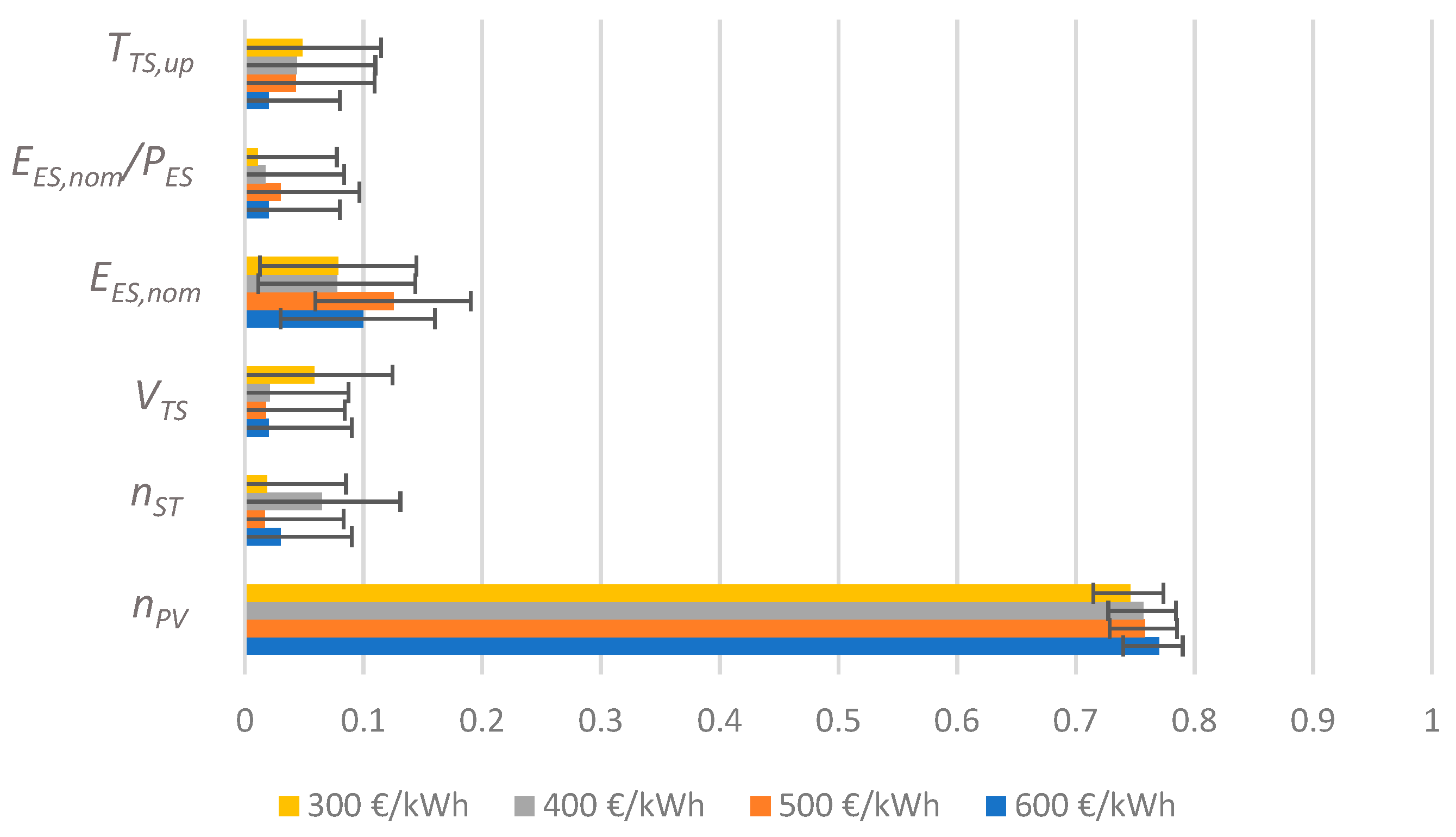
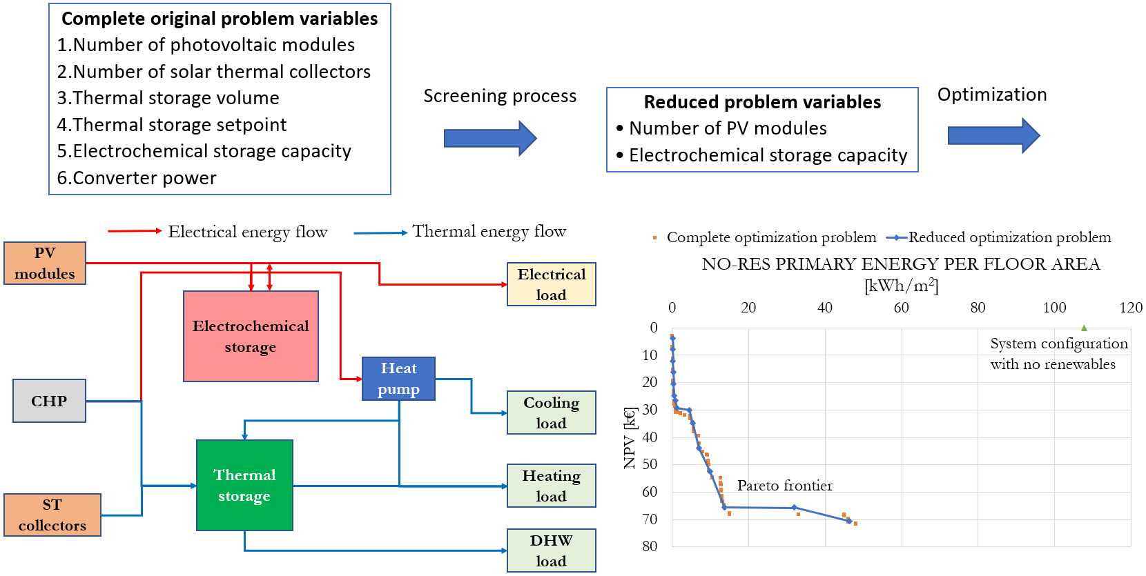
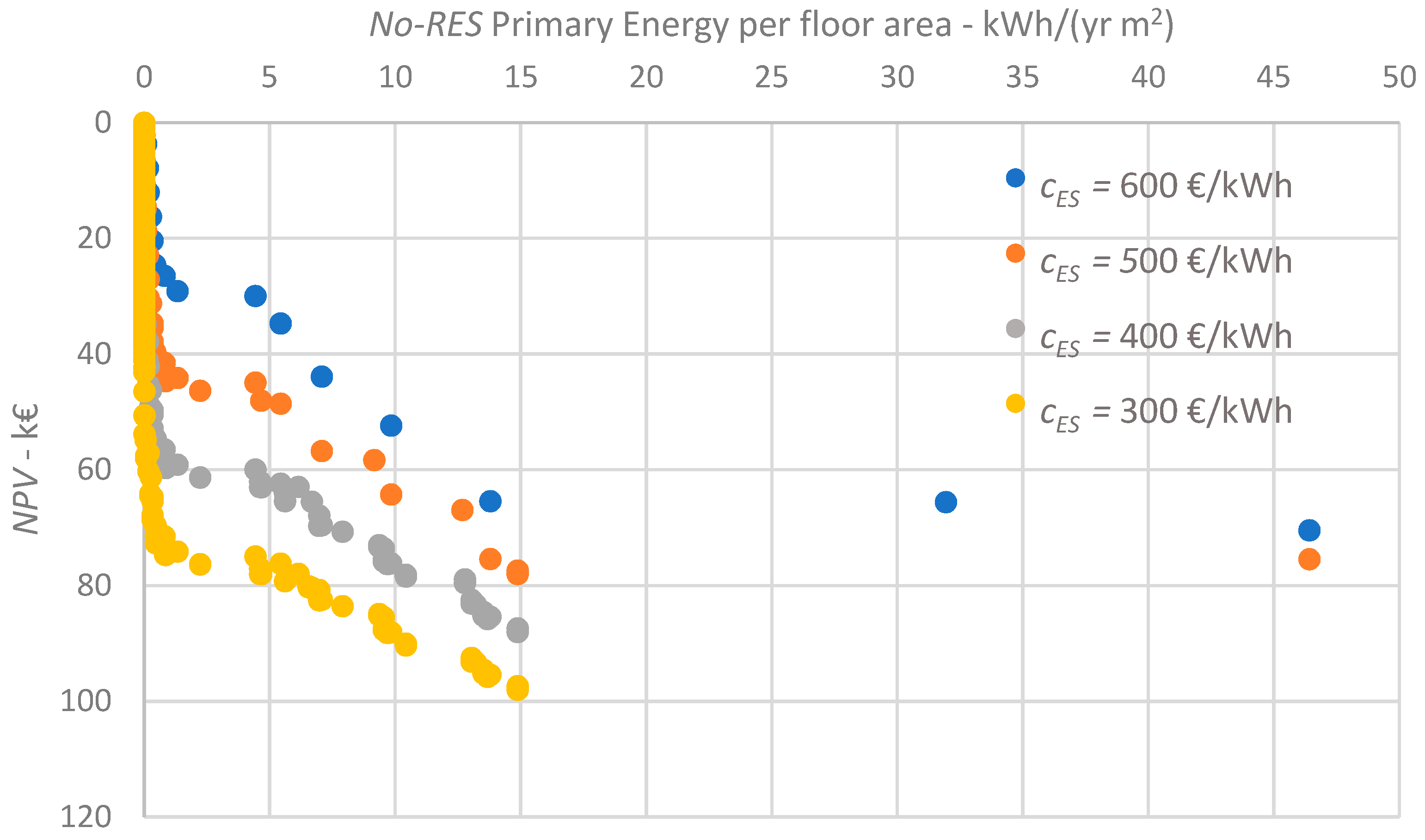
Figure 16 and Figure 17 show the correlation coefficient for $PrE{n}_{S_B}$ and $NPV$ depending on four different ${\tilde{c}}_{ES}^0$. The reduced prices do not change the relevance ranking of the variables; thus, the reduced two-variable optimization problem still applies. Figure 18 shows the four different Pareto frontiers: a lower ${\tilde{c}}_{ES}^0$ introduces many other configurations close to the null value of the No-RES energy consumption. In other words, many high-efficiency configurations have become economically viable due to a lower initial investment.

Table 6. Percentiles of the number of PV collectors and nominal ES capacity as a function of the unitary cost of the electrochemical storage.

Unitary Cost of the Electrochemical Storage	Number of Configurations on the Pareto Frontier	1st, 2nd, 3rd, and 4th Percentiles of ${\mathit{n}}_{\mathit{P}\mathit{V}}$				1st, 2nd, 3rd, and 4th Percentiles of ${\mathbf{E}}_{\mathbf{E}\mathbf{S},\mathbf{n}\mathbf{o}\mathbf{m}}$ kWh
600 €/kWh	15	72.5	120	157.5	190	100	150	150	150
500 €/kWh	19	90	140	162.5	200	112.5	150	150	200
400 €/kWh	22	90	145	160	180	150	150	200	250
300 €/kWh	36	125	150	165	200	150	250	300	400

shows the distribution of the two main design variables, $n_{PV}$ and ${\tilde{C}}_{ES}^0$, as a function of the electrochemical storage price. As mentioned above, a lower ${\tilde{c}}_{ES}^0$ moves the distribution towards higher values of both PV modules and electrochemical storage size.

The ES unitary price does not affect much the optimal range of the ratio between the nominal electrochemical storage capacity and the PV capacity (see Figure 19). Only the lowest price scenario, ${\tilde{c}}_{ES}^0=300 €/\mathrm{kWh}$, makes the installation of larger ES viable. However, the general criterion of 4–8 h seems a robust guideline.

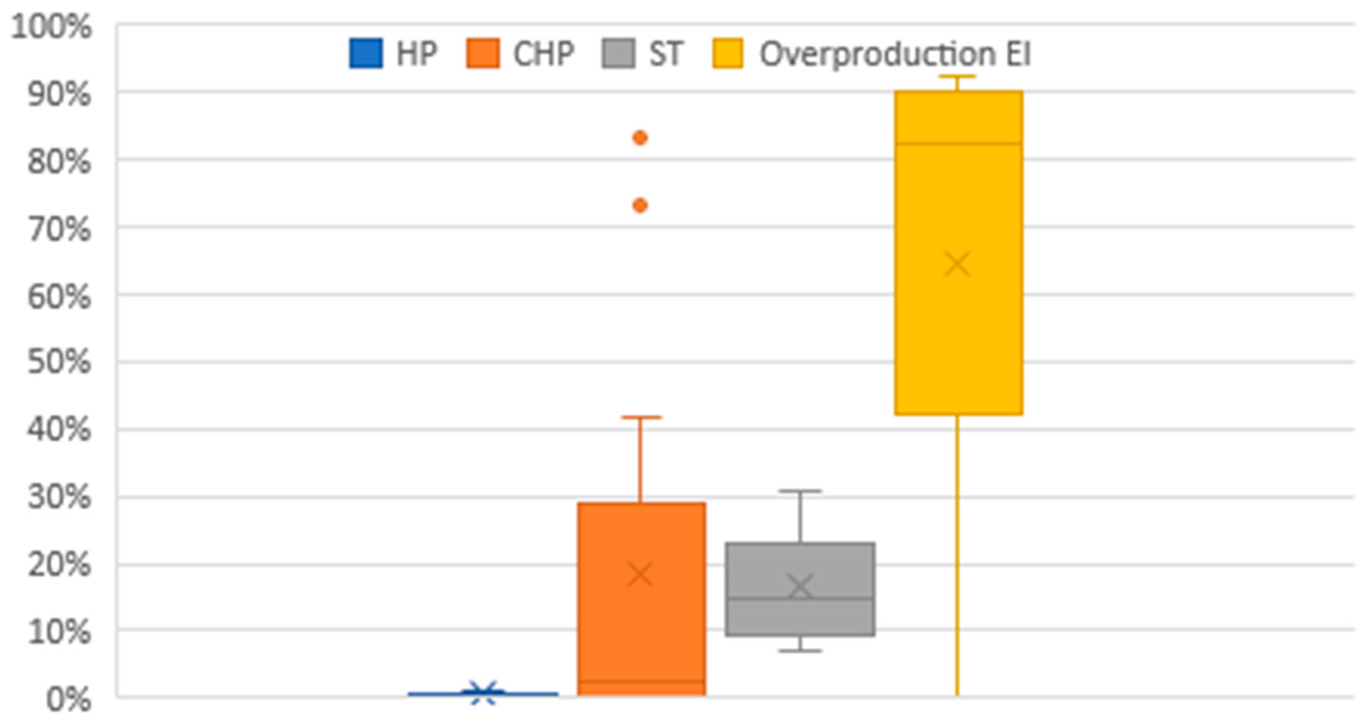
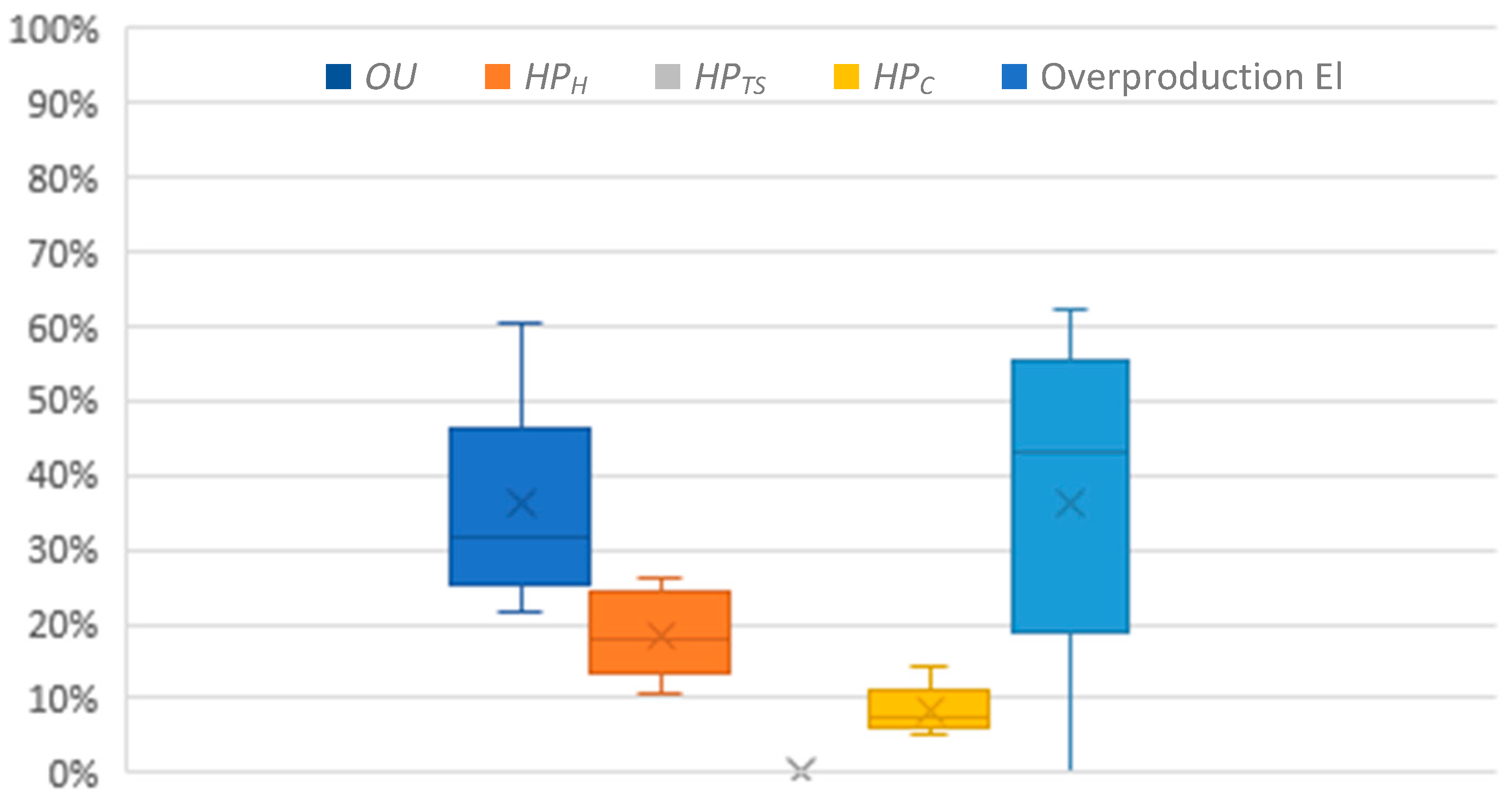
Figure 20 shows that the electrical overproduction does not reduce with lower ${\tilde{c}}_{ES}^0$, as the more favorable economic context increases the size of the electrochemical storage, but also increases the number of PV modules. Figure 21 shows the median value of the $So{C}_{ES}$ of the configurations on the Pareto frontier, as a function of the ES unitary price. We observe that the notable amount of installed PV reduces the deficit of electrical energy (Equation (6d)), resulting in low values of $\Delta So{C}_{ES}$ and high values of $So{C}_{ES}$. The latter operative condition also ensures the lifetime of the electrochemical storage, which is never replaced during the 20 years considered.

6. Conclusions

In this work, we optimized a HRES system serving a reference off-grid small-to-medium accommodation facility, according to a multi-objective perspective: the minimization of No-RES energy consumption and maximization of NPV at the end of system lifetime. After describing both energy and economic models, we showed how the multi-variable optimization problem can be simplified through a correlation analysis of a random sample of possible configurations, to identify the design variables that mainly affect the objective functions.

The methodology has been applied to a test case including air-to-water heat pumps, a combined heat-power generator, photovoltaic modules, solar thermal collectors, and electrochemical and thermal storages. The design variables have been reduced from 6 to 2 (i.e., PV number and nominal energy of the electrochemical storage) and the design alternatives from 330,000 to 220. We showed how the reduced problem does not exclude optimal configurations, since the new Pareto frontier overlaps that obtained considering all the 6 variables.

Achievable energy savings go from ~57% to ~100%, and the corresponding NPV and IRR after 20 years of operation go from ~4 k€ to ~70 k€ and from 5.2% to ~27%. Finally, we found a simple rule of thumb to design PV capacity and ES size for similar PV-driven off-grid buildings: the best ratio between the two quantities goes from 4 to 8 h, regardless the cost of the electrochemical storage. A lower price makes economically viable configurations with higher PV capacity and ES size, thus reducing the use of No-RES generators. However, the electrical overproduction is not reduced, as the optimal ratio between PV capacity and electrical storage capacity does not vary.

Next studies will concern a more detailed stochastic analysis of both technical and economic parameters, to figure out the probability distributions of the selected objective functions and thus the statistically expected performances and the worst-case scenarios, for risk-management purposes.

References

1. McGovern, T.; Hicks, C. Deregulation and restructuring of the global electricity supply industry and its impact upon power plant suppliers. Int. J. Prod. Econ. 2004, 89, 321–337. [Google Scholar] [CrossRef]
2. Jaber, J.O.; Al-Sarkhi, A.; Akash, B.A.; Mohsen, M.S. Medium-range planning economics of future electrical-power generation options. Energy Policy 2004, 32, 357–366. [Google Scholar] [CrossRef]
3. Nfah, E.M.; Ngundam, J.M.; Vandenbergh, M.; Schmid, J. Simulation of off-grid generation options for remote villages in Cameroon. Renew. Energy 2008, 33, 1064–1072. [Google Scholar] [CrossRef]
4. Conti, P.; Schito, E.; Testi, D. Cost-Benefit Analysis of Hybrid Photovoltaic/Thermal Collectors in a Nearly Zero-Energy Building. Energies 2019, 12, 1582. [Google Scholar] [CrossRef]
5. Testi, D.; Conti, P.; Schito, E.; Urbanucci, L.; D’Ettorre, F. Synthesis and Optimal Operation of Smart Microgrids Serving a Cluster of Buildings on a Campus with Centralized and Distributed Hybrid Renewable Energy Units. Energies 2019, 12, 745. [Google Scholar] [CrossRef]
6. Bilal, B.O.; Sambou, V.; Ndiaye, P.A.; Kébé, C.M.F.; Ndongo, M. Optimal design of a hybrid solar e wind—Battery system using the minimization of the annualized cost system and the minimization of the loss of power supply probability (LPSP). Renew. Energy 2010, 35, 2388–2390. [Google Scholar] [CrossRef]
7. Kalantar, M.; Mousavi, S.M.G. Dynamic behavior of a stand-alone hybrid power generation system of wind turbine, microturbine, solar array and battery storage. Appl. Energy 2010, 87, 3051–3064. [Google Scholar] [CrossRef]
8. Fadaee, M.; Radzi, M.A.M. Multi-objective optimization of a stand-alone hybrid renewable energy system by using evolutionary algorithms: A review. Renew. Sustain. Energy Rev. 2012, 16, 3364–3369. [Google Scholar] [CrossRef]
9. Alsayed, M.; Cacciato, M.; Scarcella, G.; Scelba, G. Multicriteria Optimal Sizing of Photovoltaic-Wind Turbine Grid Connected Systems. IEEE Trans. Energy Convers. 2013, 28, 370–379. [Google Scholar] [CrossRef]
10. Urbanucci, L.; Testi, D. Optimal integrated sizing and operation of a CHP system with Monte Carlo risk analysis for long-term uncertainty in energy demands. Energy Convers. Manag. 2018, 157, 307–316. [Google Scholar] [CrossRef]
11. Zhou, W.; Lou, C.; Li, Z.; Lu, L.; Yang, H. Current status of research on optimum sizing of stand-alone hybrid solar–wind power generation systems. Appl. Energy 2010, 87, 380–389. [Google Scholar] [CrossRef]
12. Schito, E.; Conti, P.; Testi, D. Multi-objective optimization of microclimate in museums for concurrent reduction of energy needs, visitors’ discomfort and artwork preservation risks. Appl. Energy 2018, 224, 147–159. [Google Scholar] [CrossRef]
13. Grassi, W.; Conti, P.; Schito, E.; Testi, D. Solutions to Improve Energy Efficiency in HVAC for Renovated Buildings (Chapter 9.3). In Handbook of Energy Efficiency in Buildings; Asdrubali, F., Desideri, U., Eds.; Elsevier: Amsterdam, The Netherlands, 2019; pp. 675–810. [Google Scholar]
14. D’Ettorre, F.; Conti, P.; Schito, E.; Testi, D. Model predictive control of a hybrid heat pump system and impact of the prediction horizon on cost-saving potential and optimal storage capacity. Appl. Therm. Eng. 2019, 148, 524–535. [Google Scholar] [CrossRef]
15. Grassi, W.; Conti, P.; Schito, E.; Testi, D. On sustainable and efficient design of ground-source heat pump systems. J. Phys. Conf. Ser. 2015, 655, 012003. [Google Scholar] [CrossRef]
16. Bernal-Agustín, J.L.; Dufo-López, R. Simulation and optimization of stand-alone hybrid renewable energy systems. Renew. Sustain. Energy Rev. 2009, 13, 2111–2118. [Google Scholar] [CrossRef]
17. Fioriti, D.; Giglioli, R.; Poli, D.; Lutzemberger, G.; Vanni, A.; Salza, P. Optimal sizing of a hybrid mini-grid considering the fuel procurement and a rolling horizon system operation. In Proceedings of the 2017 IEEE International Conference on Environment and Electrical Engineering and 2017 IEEE Industrial and Commercial Power Systems Europe (EEEIC/I&CPS Europe), Milan, Italy, 6–9 June 2017; pp. 1–6. [Google Scholar]
18. Fioriti, D.; Giglioli, R.; Poli, D.; Lutzemberger, G.; Micangeli, A.; Del Citto, R.; Perez-Arriaga, I.; Duenas-Martinez, P. Stochastic sizing of isolated rural mini-grids, including effects of fuel procurement and operational strategies. Electr. Power Syst. Res. 2018, 160, 419–428. [Google Scholar] [CrossRef] [Green Version]
19. Faccio, M.; Gamberi, M.; Bortolini, M.; Nedaei, M. State-of-art review of the optimization methods to design the configuration of hybrid renewable energy systems (HRESs). Front. Energy 2018, 12, 591–622. [Google Scholar] [CrossRef]
20. Siddaiah, R.; Saini, R.P. A review on planning, configurations, modeling and optimization techniques of hybrid renewable energy systems for off grid applications. Renew. Sustain. Energy Rev. 2016, 58, 376–396. [Google Scholar] [CrossRef]
21. Rong, A.; Su, Y. Polygeneration systems in buildings: A survey on optimization approaches. Energy Build. 2017, 151, 439–454. [Google Scholar] [CrossRef]
22. Abdmouleh, Z.; Gastli, A.; Ben-Brahim, L.; Haouari, M.; Al-Emadi, N.A. Review of optimization techniques applied for the integration of distributed generation from renewable energy sources. Renew. Energy 2017, 113, 266–280. [Google Scholar] [CrossRef]
23. Frangopoulos, C.A. Recent developments and trends in optimization of energy systems. Energy 2018, 164, 1011–1020. [Google Scholar] [CrossRef]
24. Waibel, C.; Wortmann, T.; Evins, R.; Carmeliet, J. Building energy optimization: An extensive benchmark of global search algorithms. Energy Build. 2019, 187, 218–240. [Google Scholar] [CrossRef]
25. Montgomery, D.C. Design and Analysis of Experiments, 9th ed.; John Wiley & Sons, Inc.: Hoboken, NJ, USA, 2017. [Google Scholar]
26. Uy, M.; Telford, J.K. Optimization by Design of Experiment techniques. In Proceedings of the 2009 IEEE Aerospace Conference, Big Sky, MT, USA, 7–14 March 2009; pp. 1–10. [Google Scholar]
27. International Organization for Standardization. ISO 13786, Thermal Performance of Building Components—Dynamic Thermal Characteristics—Calculation Methods; International Organization for Standardization: Geneva, Switzerland, 2017; p. 19. [Google Scholar]
28. Testi, D.; Schito, E.; Conti, P. Cost-optimal Sizing of Solar Thermal and Photovoltaic Systems for the Heating and Cooling Needs of a Nearly Zero-energy Building: Design Methodology and Model Description. Energy Procedia 2016, 91, 517–527. [Google Scholar] [CrossRef]
29. O’Callaghan, P.W.; Probert, S.D. Sol-air temperature. Appl. Energy 1977, 3, 307–311. [Google Scholar] [CrossRef]
30. Aprile, M. Energetic characterization of the hotel sector in Italy. Available online: http://progettoegadi.enea.it/it/RSE162.pdf (accessed on 2 August 2019).
31. Testi, D.; Schito, E.; Conti, P. Cost-optimal Sizing of Solar Thermal and Photovoltaic Systems for the Heating and Cooling Needs of a Nearly Zero-Energy Building: The Case Study of a Farm Hostel in Italy. Energy Procedia 2016, 91, 528–536. [Google Scholar] [CrossRef]
32. Duffie, J.A.; Beckman, W.A. Solar Engineering of Thermal Processes, 4th ed.; John Wiley & Sons, Inc.: Hoboken, NJ, USA, 2013. [Google Scholar]
33. Evans, D.L. Simplified method for predicting photovoltaic array output. Sol. Energy 1981, 27, 555–560. [Google Scholar] [CrossRef]
34. European Committee for Standardization. (CEN) EN 12975, Thermal Solar Systems and Components—Solar Collectors—Part 2: Test Methods; European Committee for Standardization: Brussels, Belgium, 2006. [Google Scholar]
35. European Committee for Standardization. (CEN) EN 15316-2, Energy Performance of Buildings—Method for Calculation of System Energy Requirements and System Efficiencies—Part 2: Space Emission Systems (Heating and Cooling); European Committee for Standardization: Brussels, Belgium, 2017. [Google Scholar]
36. Ecker, M.; Nieto, N.; Käbitz, S.; Schmalstieg, J.; Blanke, H.; Warnecke, A.; Sauer, D.U. Calendar and cycle life study of Li(NiMnCo)O2-based 18650 lithium-ion batteries. J. Power Sources 2014, 248, 839–851. [Google Scholar] [CrossRef]
37. Omar, N.; Monem, M.A.; Firouz, Y.; Salminen, J.; Smekens, J.; Hegazy, O.; Gaulous, H.; Mulder, G.; Van den Bossche, P.; Coosemans, T.; et al. Lithium iron phosphate based battery—Assessment of the aging parameters and development of cycle life model. Appl. Energy 2014, 113, 1575–1585. [Google Scholar] [CrossRef]
38. Park, J.; Appiah, W.A.; Byun, S.; Jin, D.; Ryou, M.H.; Lee, Y.M. Semi-empirical long-term cycle life model coupled with an electrolyte depletion function for large-format graphite/LiFePO4 lithium-ion batteries. J. Power Sources 2017, 365, 257–265. [Google Scholar] [CrossRef]
39. A123 Official Site. Available online: http://www.a123systems.com (accessed on 2 August 2019).
40. Rao, S.S. Engineering Optimization: Theory and Practice, 3rd ed.; John Wiley & Sons, Inc.: Hoboken, NJ, USA, 1996. [Google Scholar]
41. Spiegel, M.R.; Stephens, L.J. Schaum’s Outline of Statistics, 4th ed.; McGraw-Hill: New York, NY, USA, 2007. [Google Scholar]
42. CTI (Italian Thermotecnical Committee) Italian Typical Meteorological Years. Available online: https://www.cti2000.it (accessed on 2 August 2019).
43. Ceraolo, M.; Giglioli, R.; Lutzemberger, G.; Bechini, A. Cost effective storage for energy saving in feeding systems of tramways. In Proceedings of the 2014 IEEE International Electric Vehicle Conference (IEVC), Florence, Italy, 17–19 December 2014; pp. 1–6. [Google Scholar]
44. Kokam Battery. Available online: http://kokam.com/cell (accessed on 2 August 2019).
45. Winston Battery. Available online: http://en.winston-battery.com (accessed on 2 August 2019).
Figure 1. Schematization of the overall building system.
Energies 12 03026 g001
Figure 2. Number of allowed charging-discharging cycles vs. depth of discharge.
Energies 12 03026 g002
Figure 3. Pareto frontiers of the full (477 points) and reduced (15 points) optimization problems. The No-RES configuration is shown with a green marker.
Energies 12 03026 g003
Figure 4. Number of photovoltaic (PV) modules for the configurations on the Pareto Frontier.
Energies 12 03026 g004
Figure 5. Nominal electrochemical storage (ES) energy for the configurations on the Pareto Frontier.
Energies 12 03026 g005
Figure 6. Energy consumption and net present value as a function of the number of PV modules on the Pareto frontier.
Energies 12 03026 g006
Figure 7. Energy consumption and net present value as a function of the nominal ES energy on the Pareto frontier.
Energies 12 03026 g007
Figure 8. Internal rate of return (IRR) and initial cost as a function of the number of PV modules number.
Energies 12 03026 g008
Figure 9. IRR and initial cost as a function of the nominal ES capacity.
Energies 12 03026 g009
Figure 10. Box and whisker plot of the heating demand percentage directly delivered by the heat pump (HP) and thermal storage (TS).
Energies 12 03026 g010
Figure 11. Box and whisker plot of the energy percentage delivered to the thermal storage by the different sources.
Energies 12 03026 g011
Figure 12. Box and whisker plot of the percentage of the thermal storage losses, overproduction, domestic hot water (DHW), and heating output with respect to the total energy input.
Energies 12 03026 g012
Figure 13. Box and whisker plot of the electrical production percentage by the PV modules and CHP unit.
Energies 12 03026 g013
Figure 14. Box and whisker plot of the mean and median values of the S o C E S .
Energies 12 03026 g014
Figure 15. Box and whisker plot of the percentage of the electrical uses with respect to the total electricity production.
Energies 12 03026 g015
Figure 16. Correlation coefficient between the design variables and the No-RES (renewable energy sources) primary energy consumption, depending on ES unitary price.
Energies 12 03026 g016
Figure 17. Correlation coefficient between the design variables and the net present value, depending on ES unitary price.
Energies 12 03026 g017
Figure 18. Sensitivity analysis of the Pareto frontier depending on the ES unitary cost.
Energies 12 03026 g018
Figure 19. Ratio between the nominal electrochemical storage capacity and the PV capacity depending on ES unitary price.
Energies 12 03026 g019
Figure 20. Box and whisker plot of the percentage of the electrical overproduction with respect to the total electricity production, depending on the ES unitary cost.
Energies 12 03026 g020
Figure 21. Box and whisker plot of the median value of the electrochemical storage S o C E S , depending on the ES unitary cost.
Energies 12 03026 g021