Profit Maximizing Control of a Microgrid with Renewable Generation and BESS Based on a Battery Cycle Life Model and Energy Price Forecasting

Abstract
:
1. Introduction
1.1. Motivations
1.2. Literature Review
1.3. Contribution
2. Problem Statement
3. System Model and Costs
3.1. Microgrid Model
3.1.1. Predicted Data
3.1.2. Battery Energy Storage System
3.1.3. Power Balancing in the Microgrid
3.2. Battery Aging and Cost Models
3.2.1. Cycle Life Model
3.2.2. Counting Half Cycles
3.2.3. Cycle Life Cost Model
3.3. Redefine the Cost Model of Battery Cycle Life
4. Optimization Technique
4.1. Optimization Problem
4.2. Updating Local Extremes
5. Simulation
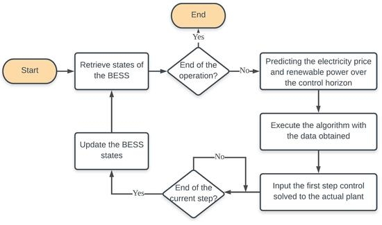
5.1. Set Up
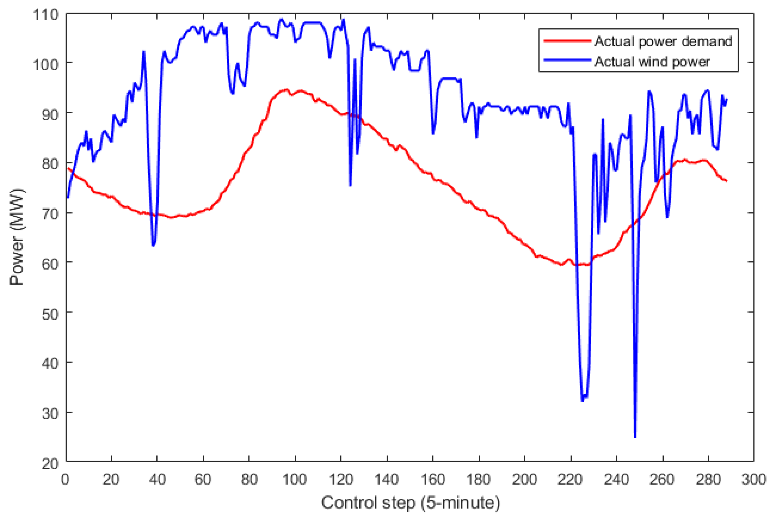
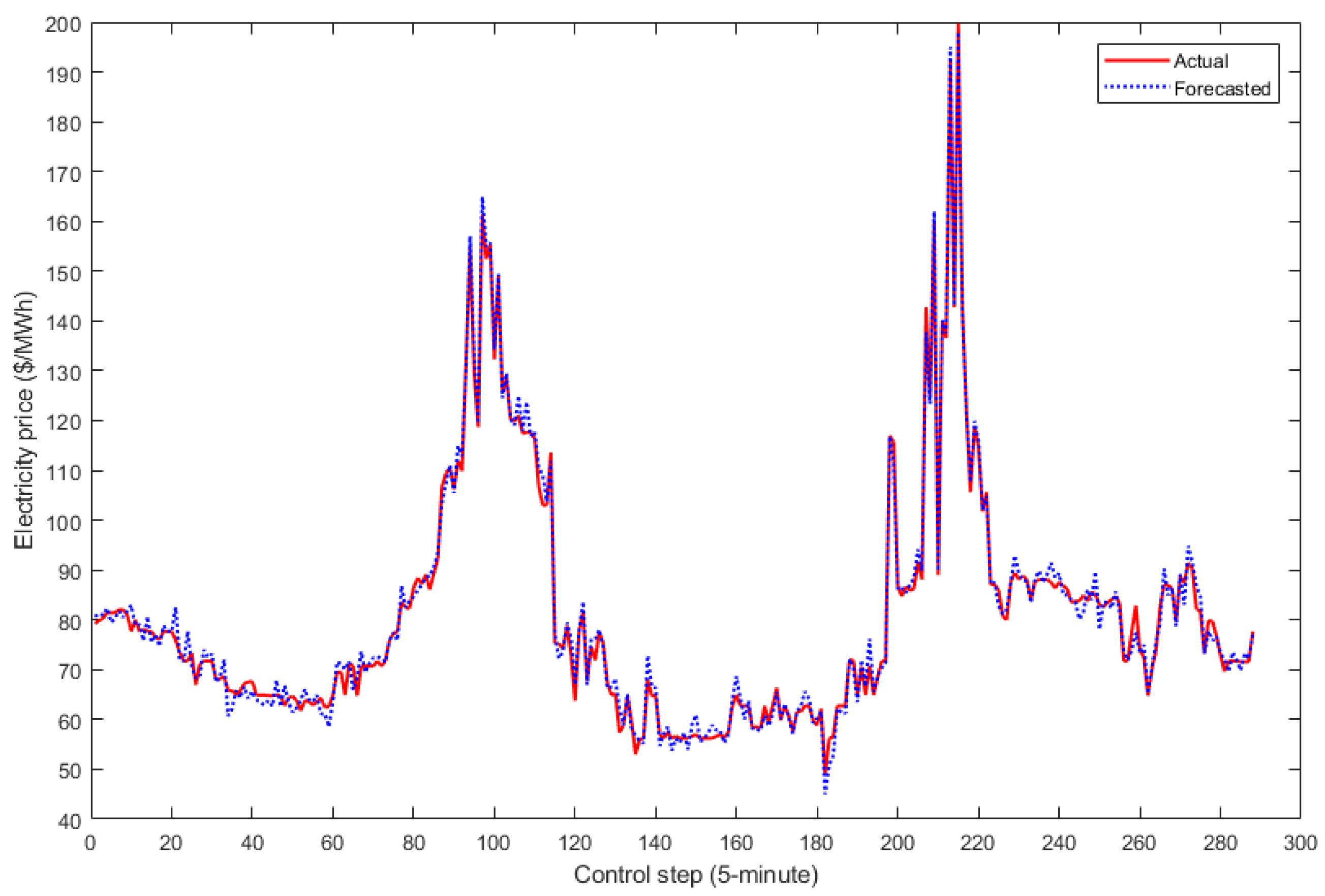
5.2. Parameters and Database
5.3. Simulation Results
5.4. Discussion
6. Conclusions
Author Contributions
Funding
Conflicts of Interest
Abbreviations
| BESS | Battery energy storage system |
| MPC | Model predictive control |
| DP | Dynamic programming |
| SMC | Sliding mode control |
| RL | Reinforcement learning |
| PSO | Particle swarm optimization |
| MILP | Mixed-integer linear programming |
| MDP | Markov decision process |
| SOC | State of charge |
| DOD | Depth of discharge |
| DE | Differential evolution |
| DG | Distributed generator |
References
- Luo, F.; Xu, Z.; Meng, K.; Dong, Z.Y. Optimal operation scheduling for microgrid with high penetrations of solar power and thermostatically controlled loads. Sci. Technol. Built Environ. 2016, 22, 666–673. [Google Scholar] [CrossRef]
- Provata, E.; Kolokotsa, D.; Papantoniou, S.; Pietrini, M.; Giovannelli, A.; Romiti, G. Development of optimization algorithms for the Leaf Community microgrid. Renew. Energy 2015, 74, 782–795. [Google Scholar] [CrossRef]
- Khalid, M.; Ahmadi, A.; Savkin, A.V.; Agelidis, V.G. Minimizing the energy cost for microgrids integrated with renewable energy resources and conventional generation using controlled battery energy storage. Renew. Energy 2016, 97, 646–655. [Google Scholar] [CrossRef]
- Zhuo, W.; Savkin, A.V.; Meng, K. Decentralized Optimal Control of a Microgrid with Solar PV, BESS and Thermostatically Controlled Loads. Energies 2019, 12, 2111. [Google Scholar] [CrossRef]
- Khalid, M.; Savkin, A.V. A model predictive control approach to the problem of wind power smoothing with controlled battery storage. Renew. Energy 2010, 35, 1520–1526. [Google Scholar] [CrossRef]
- Khalid, M.; Aguilera, R.P.; Savkin, A.V.; Agelidis, V.G. A market-oriented wind power dispatch strategy using adaptive price thresholds and battery energy storage. Wind Energy 2018, 21, 242–254. [Google Scholar] [CrossRef]
- Khalid, M.; Aguilera, R.P.; Savkin, A.V.; Agelidis, V.G. On maximizing profit of wind-battery supported power station based on wind power and energy price forecasting. Appl. Energy 2018, 211, 764–773. [Google Scholar] [CrossRef]
- Khalid, M.; Savkin, A.V. An optimal operation of wind energy storage system for frequency control based on model predictive control. Renew. Energy 2012, 48, 127–132. [Google Scholar] [CrossRef]
- Ji, Y.; Wang, J.; Xu, J.; Fang, X.; Zhang, H. Real-Time Energy Management of a Microgrid Using Deep Reinforcement Learning. Energies 2019, 12, 2291. [Google Scholar] [CrossRef]
- Bui, V.H.; Hussain, A.; Kim, H.M. Q-Learning-Based Operation Strategy for Community Battery Energy Storage System (CBESS) in Microgrid System. Energies 2019, 12, 1789. [Google Scholar] [CrossRef]
- Wu, X.; Cao, W.; Wang, D.; Ding, M. A Multi-Objective Optimization Dispatch Method for Microgrid Energy Management Considering the Power Loss of Converters. Energies 2019, 12, 2160. [Google Scholar] [CrossRef]
- Nikolovski, S.; Reza Baghaee, H.; Mlakić, D. ANFIS-based Peak Power Shaving/Curtailment in Microgrids including PV Units and BESSs. Energies 2018, 11, 2953. [Google Scholar] [CrossRef]
- Wang, D.; Qiu, J.; Reedman, L.; Meng, K.; Lai, L.L. Two-stage energy management for networked microgrids with high renewable penetration. Appl. Energy 2018, 226, 39–48. [Google Scholar] [CrossRef]
- Parisio, A.; Rikos, E.; Glielmo, L. A model predictive control approach to microgrid operation optimization. IEEE Trans. Control Syst. Technol. 2014, 22, 1813–1827. [Google Scholar] [CrossRef]
- Gu, W.; Wang, Z.; Wu, Z.; Luo, Z.; Tang, Y.; Wang, J. An online optimal dispatch schedule for CCHP microgrids based on model predictive control. IEEE Trans. Smart Grid 2016, 8, 2332–2342. [Google Scholar] [CrossRef]
- Levron, Y.; Guerrero, J.M.; Beck, Y. Optimal power flow in microgrids with energy storage. IEEE Trans. Power Syst. 2013, 28, 3226–3234. [Google Scholar] [CrossRef]
- Baghaee, H.R.; Mirsalim, M.; Gharehpetian, G.B.; Talebi, H.A. Decentralized sliding mode control of WG/PV/FC microgrids under unbalanced and nonlinear load conditions for on-and off-grid modes. IEEE Syst. J. 2017, 12, 3108–3119. [Google Scholar] [CrossRef]
- Baghaee, H.R.; Mirsalim, M.; Gharehpetian, G.B.; Talebi, H.A. A decentralized power management and sliding mode control strategy for hybrid AC/DC microgrids including renewable energy resources. IEEE Trans. Ind. Inform. 2017. [Google Scholar] [CrossRef]
- Baghaee, H.R.; Mirsalim, M.; Gharehpetian, G.B. Multi-objective optimal power management and sizing of a reliable wind/PV microgrid with hydrogen energy storage using MOPSO. J. Intell. Fuzzy Syst. 2017, 32, 1753–1773. [Google Scholar] [CrossRef]
- Baghaee, H.; Mirsalim, M.; Gharehpetian, G.; Talebi, H. Reliability/cost-based multi-objective Pareto optimal design of stand-alone wind/PV/FC generation microgrid system. Energy 2016, 115, 1022–1041. [Google Scholar] [CrossRef]
- Kaviani, A.K.; Baghaee, H.R.; Riahy, G.H. Optimal sizing of a stand-alone wind/photovoltaic generation unit using particle swarm optimization. Simulation 2009, 85, 89–99. [Google Scholar] [CrossRef]
- He, G.; Chen, Q.; Kang, C.; Pinson, P.; Xia, Q. Optimal bidding strategy of battery storage in power markets considering performance-based regulation and battery cycle life. IEEE Trans. Smart Grid 2015, 7, 2359–2367. [Google Scholar] [CrossRef]
- Xu, B.; Oudalov, A.; Ulbig, A.; Andersson, G.; Kirschen, D.S. Modeling of lithium-ion battery degradation for cell life assessment. IEEE Trans. Smart Grid 2016, 9, 1131–1140. [Google Scholar] [CrossRef]
- Vetter, J.; Novák, P.; Wagner, M.R.; Veit, C.; Möller, K.C.; Besenhard, J.; Winter, M.; Wohlfahrt-Mehrens, M.; Vogler, C.; Hammouche, A. Ageing mechanisms in lithium-ion batteries. J. Power Sources 2005, 147, 269–281. [Google Scholar] [CrossRef]
- Xu, B.; Zhao, J.; Zheng, T.; Litvinov, E.; Kirschen, D.S. Factoring the cycle aging cost of batteries participating in electricity markets. IEEE Trans. Power Syst. 2017, 33, 2248–2259. [Google Scholar] [CrossRef]
- Morstyn, T.; Savkin, A.V.; Hredzak, B.; Agelidis, V.G. Multi-agent sliding mode control for state of charge balancing between battery energy storage systems distributed in a DC microgrid. IEEE Trans. Smart Grid 2017, 9, 4735–4743. [Google Scholar] [CrossRef]
- Sideratos, G.; Hatziargyriou, N.D. An advanced statistical method for wind power forecasting. IEEE Trans. Power Syst. 2007, 22, 258–265. [Google Scholar] [CrossRef]
- Khalid, M.; Savkin, A.V. A method for short-term wind power prediction with multiple observation points. IEEE Trans. Power Syst. 2012, 27, 579–586. [Google Scholar] [CrossRef]
- Bellman, R. Dynamic Programming; Princeton University Press: Princeton, NJ, USA, 2010. [Google Scholar]
- Bertsekas, D.P. Dynamic Programming and Optimal Control; Athena Scientific: Belmont, MA, USA, 1995. [Google Scholar]
- Lee, K.Y.; Park, J.B. Application of particle swarm optimization to economic dispatch problem: Advantages and disadvantages. In Proceedings of the 2006 IEEE PES Power Systems Conference and Exposition, Atlanta, GA, USA, 29 October–1 November 2006; IEEE: Piscataway, NJ, USA, 2006; pp. 188–192. [Google Scholar]
- Guerrero, J.M.; Chandorkar, M.; Lee, T.L.; Loh, P.C. Advanced control architectures for intelligent microgrids—Part I: Decentralized and hierarchical control. IEEE Trans. Ind. Electron. 2012, 60, 1254–1262. [Google Scholar] [CrossRef]
- Guerrero, J.M.; Vasquez, J.C.; Matas, J.; De Vicuña, L.G.; Castilla, M. Hierarchical control of droop-controlled AC and DC microgrids—A general approach toward standardization. IEEE Trans. Ind. Electron. 2010, 58, 158–172. [Google Scholar] [CrossRef]
- Baghaee, H.R.; Mirsalim, M.; Gharehpetian, G.B. Real-time verification of new controller to improve small/large-signal stability and fault ride-through capability of multi-DER microgrids. IET Gener. Transm. Distrib. 2016, 10, 3068–3084. [Google Scholar] [CrossRef]
- Baghaee, H.R.; Mirsalim, M.; Gharehpetian, G.B. Performance improvement of multi-DER microgrid for small-and large-signal disturbances and nonlinear loads: Novel complementary control loop and fuzzy controller in a hierarchical droop-based control scheme. IEEE Syst. J. 2016, 12, 444–451. [Google Scholar] [CrossRef]
- Baghaee, H.R.; Mirsalim, M.; Gharehpetian, G.B.; Talebi, H.A. Eigenvalue, robustness and time delay analysis of hierarchical control scheme in multi-DER microgrid to enhance small/large-signal stability using complementary loop and fuzzy logic controller. J. Circuits Syst. Comput. 2017, 26, 1750099. [Google Scholar] [CrossRef]
- Baghaee, H.R.; Mirsalim, M.; Gharehpetian, G.B. Power calculation using RBF neural networks to improve power sharing of hierarchical control scheme in multi-DER microgrids. IEEE J. Emerg. Sel. Top. Power Electron. 2016, 4, 1217–1225. [Google Scholar] [CrossRef]


| 24 MW | 60 MW | 1.25 MWh | 11.25 MWh | 12.5 MWh | 2,500,000 $ |
| kp | d | n | ||
|---|---|---|---|---|
| 2347 | 1.1 | 1/12 | 0.05 | 5 |
| BESS Cost | Energy Trading Cost | Overall Cost | Cost without BESS | |
|---|---|---|---|---|
| Higher demand | 3849.07 | 410,851.24 | 414,700.31 | 433,108.81 |
| Lower demand | 2548.24 | −394,509.25 | −391,961.01 | −369,880.45 |
© 2019 by the authors. Licensee MDPI, Basel, Switzerland. This article is an open access article distributed under the terms and conditions of the Creative Commons Attribution (CC BY) license (http://creativecommons.org/licenses/by/4.0/).
Share and Cite
Zhuo, W.; Savkin, A.V. Profit Maximizing Control of a Microgrid with Renewable Generation and BESS Based on a Battery Cycle Life Model and Energy Price Forecasting. Energies 2019, 12, 2904. https://doi.org/10.3390/en12152904
Zhuo W, Savkin AV. Profit Maximizing Control of a Microgrid with Renewable Generation and BESS Based on a Battery Cycle Life Model and Energy Price Forecasting. Energies. 2019; 12(15):2904. https://doi.org/10.3390/en12152904
Chicago/Turabian StyleZhuo, Wenhao, and Andrey V. Savkin. 2019. "Profit Maximizing Control of a Microgrid with Renewable Generation and BESS Based on a Battery Cycle Life Model and Energy Price Forecasting" Energies 12, no. 15: 2904. https://doi.org/10.3390/en12152904